Model of Bio-Colonisation on Mooring Lines: Updating Strategy Based on a Static Qualifying Sea State for Floating Wind Turbines - MDPI
←
→
Page content transcription
If your browser does not render page correctly, please read the page content below
Journal of
           Marine Science
           and Engineering

Article
Model of Bio-Colonisation on Mooring Lines:
Updating Strategy Based on a Static Qualifying Sea
State for Floating Wind Turbines
Benjamin Decurey 1, *,† , Franck Schoefs 1,2 , Anne-Laure Barillé 3 and Thomas Soulard 2,4
 1    Institut de Recherche en Génie Civil et Mécanique (GeM)—UMR CNRS 6183, Ecole Centrale de Nantes et
      Université de Nantes, 44322 Nantes, France; Franck.Schoefs@univ-nantes.fr
 2    Institut Universitaire Mer et Littoral (IUML)—FR CNRS 3473, Université de Nantes, 44322 Nantes, France;
      thomas.soulard@ec-nantes.fr
 3    BIO-LITTORAL, 2 Rue du Château de l’Eraudière, Immeuble Le Nevada, CS 80693,
      44306 Nantes CEDEX 3, France; al.barille@bio-littoral.fr
 4    Laboratoire de recherche en Hydrodynamique, Énergétique et Environnement Atmosphérique
      (LHEEA)—UMR CNRS 6598, Ecole Centrale de Nantes, 44321 Nantes, France
 *    Correspondence: Benjamin.Decurey@univ-nantes.fr
 †    Current address: Département de Physique, Université de Nantes—UFR Sciences et Techniques,
      2 Chemin de la Houssinière, 44322 Nantes, France.

 Received: 10 January 2020; Accepted: 30 January 2020; Published: 11 February 2020

 Abstract: Bio-colonisation affects the ageing of materials and the behaviour of offshore structures.
 Mooring systems and umbilicals belong to the family of slender bodies which are components
 sensitive to bio-colonisation because of a change of dynamic behaviour due to shape, roughness
 and mass modifications. However, this stochastic process in time and space is hard to predict.
 The purpose is then twofold: first, to provide a stochastic spatial model of the bio-colonisation on
 a mooring line; second, to show that in some defined environmental conditions, such as low wave
 height, low wind and current velocities, the monitoring of mooring lines tension can help to assess
 and reduce uncertainty on this model. Therefore, a comprehensive stochastic modelling based on
 mussels colonisation was carried out using on-site videotapes, experimental campaigns and expert
 knowledge. We studied the efficiency of a virtual sensing network using this model and a conditional
 entropy metric. It is first shown that the spatial model fits well with experimental data, and second
 that a denser medium accuracy sensor network is to be preferred to a single high accuracy fairlead
 sensor to reduce the uncertainty on the model parameters. It is then worth updating bio-colonisation
 on mooring lines during the life-time of a floating wind turbine.

 Keywords: floating wind turbine; mooring line; bio-colonisation; monitoring; entropy metric

1. Introduction
     Depending on the floater’s type, the mooring system’s main function is stationkeeping and/or
stability of the floating wind turbine during its entire lifetime: 25 years or more. However,
from commissioning, and even before, to decommissioning, sources and factors of premature failure
are numerous. Nevertheless, Fontaine et al. [1], in an industry survey, showed that almost half of their
surveyed failure events were associated with fatigue and corrosion degradations, thus advising for a
better “management of mooring integrity” in this regard.
     The lifetime consumed during limited events in time, such as impacts and storms, cannot be
accurately predicted. In an offshore context, where operations are expensive and the cost of safety
factors is high, one of today’s challenges in mooring lines is to develop preventive methods [2,3] to

J. Mar. Sci. Eng. 2020, 8, 108; doi:10.3390/jmse8020108                           www.mdpi.com/journal/jmse
J. Mar. Sci. Eng. 2020, 8, 108                                                                              2 of 31

reduce prior uncertainties on the lifetime consumed by everyday action of waves, current, wind and
bio-colonisation to estimate mooring line’s state before a storm for example. However, because of the
latter actions’ high variability in time and space, deterministic models fail in accurately predicting their
state. Monitoring is, therefore, a valuable option to update preferred probabilistic models. This paper
aims to reduce prior uncertainties on one of these actions’ main parameters- bio-colonisation mass,
through monitoring.
      Bio-colonisation is defined as aggregates of marine organisms (seaweed, sponges, mussels, oysters,
barnacles, anemones, corals, tubeworms, etc.) on offshore industrial structures [4] (from p. 27).
      Figure 1 presents a pattern of mussels observed after one year of growth on the mooring chain of
the Biocolmar buoy of the University of Nantes during its inspection. Bio-colonisation macro-parameters
are its thickness, its density and its roughness ([5] (p. 140), [6] (p. 38)). They can vary in space and in
time along the line. By increasing roughness, external diameter and mass, bio-colonisation is increasing
quasi-static and dynamic loads of waves and current on the line. By increasing the line’s weight,
bio-colonisation is also changing the line’s buoyancy and its tension. Different researchers foresee
the following:

•     a reduction of mooring line’s minimum tension, leading to an increased risk of “slack event” [7]
      (fast tensioning of the line).
•     a reduction of line’s buoyancy, accelerating wearing by rubbing with the seabed.
•     a shift of natural frequencies towards larger periods at which the floater has larger response
      amplitudes [8].
•     an increase of effective tension’s variance [8].

       Figure 1. Colonisation of mussels on the mooring chain of the Biocolmar buoy of Nantes University.

     All these effects lead to a decrease of mooring lines’ lifetime [9] and an increase of uncertainties
on damages [10].
     To quantify the benefit of monitoring on uncertainty reduction, a prior stochastic model of
bio-colonisation along a mooring line has to be derived. Even if bio-colonisation is a stochastic spatial
and temporal problem with large uncertainties, previous works highlighted some trends in space and
time. Jusoh and Wolfram [11] showed a clear decrease with depth and Ameryoun [4] (from p. 45)
reviewed studies from North Atlantic offshore platforms highlighting an increase with time, limited
by natural barriers. Boukinda [12] showed long term evolution with depth for a number of species
in the Gulf of Guinea. A model is then worth. In this paper, only a stochastic spatial model will be
presented and validated against experimental data.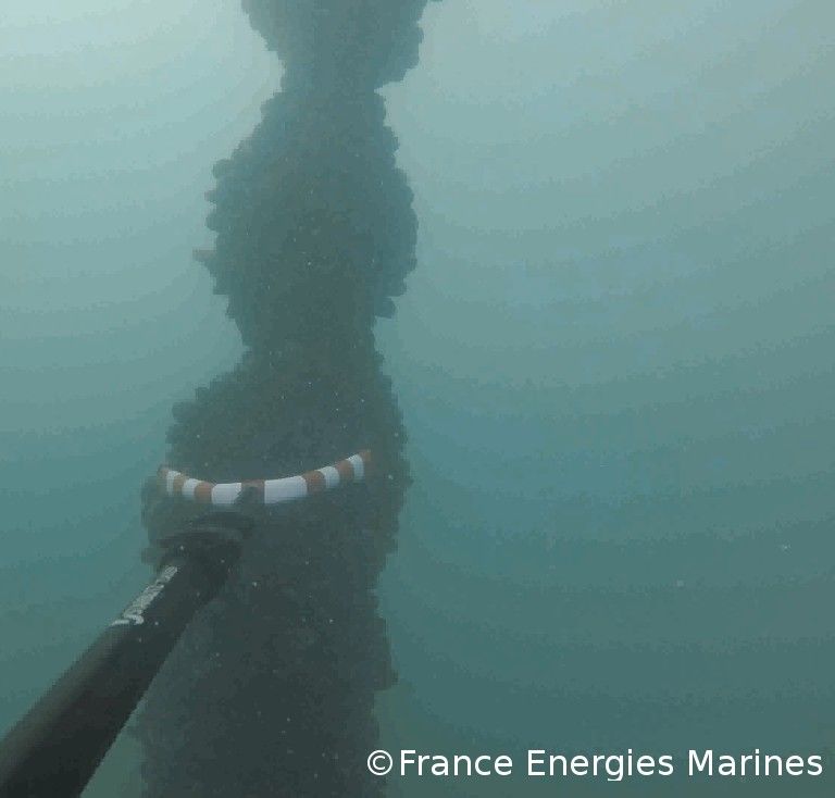
J. Mar. Sci. Eng. 2020, 8, 108 3 of 31
Because the temporal and spatial variations of bio-colonisation affect the ageing of immersed
offshore components [4], Structural Health Monitoring (SHM) is foreseen as a powerful mean to reduce
uncertainties. Because the stochastic spatial model has an a priori entropy, which could be understood
as a variability, interest of the monitoring is indeed to reduce this entropy by giving indirect information
about the real distribution, e.g., mass distribution, throughout the mooring lifetime, at appropriate
moments such as calm sea states. However, SHM could be costly, due to a short lifetime of sensors,
and it could also be uncertain, due to the relative accuracy of sensors. A natural question comes out:
How to choose SHM to not expensively reduce prior entropy of the stochastic spatial model and so
efficiently update the model? This update has a direct impact on the uncertainty on damages.
To address these key issues, the paper is organised as follows. An original stochastic spatial
model is presented and validated, then a methodology of selection of realistic spatial distributions
during a qualifying sea state is introduced. A sensitivity analysis on entropy reduction of the model
parameters depending on SHM choices is finally carried out, showing that a denser medium accuracy
sensor network is to be preferred to a single high accuracy fairlead sensor.
2. Materials and Methods
2.1. An a Priori Spatial Distribution of Bio-Colonisation
For structural engineers, macro-parameters of bio-colonisation are its thickness, density, and
roughness. We did not study spatial variability of roughness. Indeed, our data came from videotape
analysis and roughness is hard to measure when using pointing algorithm to extract information from
videotape frames. However, it could be done using advanced image processing algorithm such as
the work of O’Byrne et al. [13], which was not available at the time of the study. Concerning density,
expressed in kilograms per meter cube, it was hypothesised that density is homogeneous along the
mooring line. Without enough data, this questionable hypothesis is kept and agrees with recommended
practices in standards [6]. Therefore, in this paper, only a model of bio-colonisation thickness
is introduced, based on available quantitative data. Compared to the standards, recommending
to consider constant thicknesses [6], the purpose is to build a model capturing bio-colonisation
thickness evolution at a scale under one meter. Indeed, as shown by Spraul et al. [8], a non-constant
bio-colonisation thickness impacts the distribution of tension in the mooring line. For simplicity and
because available data did not enable us to consider the three-dimensionality of bio-colonisation,
this spatial model of thickness is based on the assumptions that bio-colonisation is axis-symmetric
around the mooring line and that it covers one hundred percents of the sectional circumference of the
mooring line. It means also that thickness will be described as a uni-dimensional process along the
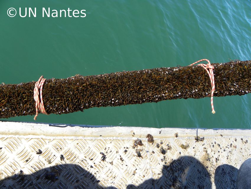
mooring line. We validated these assumptions in a recent experimental campaign for colonisation of
uni-layered mussels (cf. Figure 2). Axis-symmetry and full coverage could be observed (Figure 2) after
less than one year of colonisation.
Figure 2. Colonisation of uni-layered mussels on the mooring rope of a mussel farm.
They also agree with standards, which do not evoke any cylindrical parameterisation of
bio-colonisation for vertical or semi-vertical components.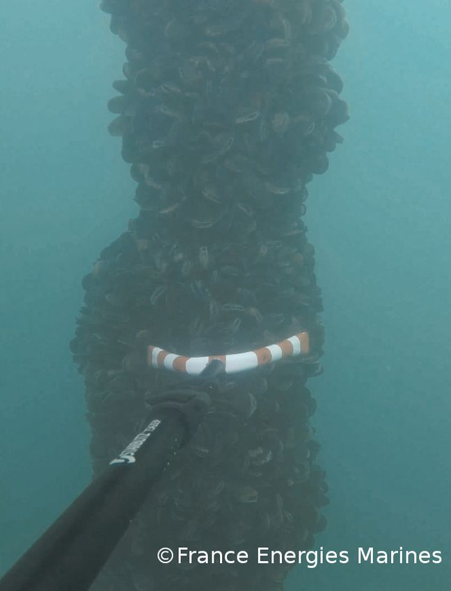
J. Mar. Sci. Eng. 2020, 8, 108                                                                              4 of 31

2.1.1. Data
      In standards [5] (p. 141) and in [14], thickness is defined as t in Figure 3.

      Figure 3. Definition of thickness (t) commonly used in standards vs. Practical measurement of thickness
      (thext ) on-site.

      However, in practice when measuring the circumference with a tape or processing a videotape
frame by pointing the outline of bio-colonisation, thext , as defined in Figure 3, is obtained. This is an
important remark because considering thickness as t or thext as an impact on the considered volume
of bio-colonisation and so on the considered range of density of bio-colonisation. In the following,
the thickness is defined as thext .
      After reviewing existing data on bio-colonisation of offshore structures, one can cite the very
large database made up during the Joint Industry R&D Project “Marine Growth Data Bank” led by
Veritec, or the work of Boukinda [12] in the Gulf of Guinea. There are still under construction large
database such as “OCEANIC” led by WavEC or “ABIOP” and “ABIOP+” which are France Energies
Marines projects. Those databases are expected to link biological observations with engineering needs.
However there is still a lack of spatially or temporally dense information. The purpose is to model
bio-colonisation at a low scale around half a meter, so spatially dense data had to be used. Therefore,
in collaboration with Centrale Nantes, already analysed (cf. Spraul et al. [8]) and new videotapes,
both from mooring chains of cardinal buoys of the SEMREV test site [15], not far from Biocolmar
(cf. Figure 1), were used to extract trajectories of bio-colonisation thickness. These videotapes were
recorded by ALPHA & CO during diving missions. The following figures, Figures 4 and 5, present
a photograph and an example of thickness trajectories of observed bio-colonisation on the mooring
chain (nominal diameter of 3, 8 cm) of the East cardinal buoy in February 2018. Please note that the
gap in the trajectory in Figure 5 is due to the fact that divers recorded some parts of the line, not all of
the line.

      Figure 4. Photograph of bio-colonisation on East cardinal buoy mooring chain of the SEMREV test site
      in February 2018.
J. Mar. Sci. Eng. 2020, 8, 108 5 of 31
Figure 5. Trajectory of the bio-colonisation thickness on East cardinal buoy mooring chain in
February 2018.
In total, three trajectories were extracted from new videotapes of two buoys and three months
apart, gathered with two already existing trajectories from Spraul et al. [8]. These trajectories are
presented in Appendix A.
It was noticed during diving missions that Mytilus edulis (mussels) is the hard species with the
highest biomass on the mooring lines of the cardinal buoys of SEMREV test site [8]. Accordingly,
the model of the bio-colonisation spatial distribution of thickness presented in this paper is suitable for
a colonisation by mussels. Instead of being a limitation, this is a benefit:
1. Mussels colonisation is a so-called hard macro-colonisation. The fluid interaction with a solid
body, instead of a soft body, can be modelled through the Morison equation.
2. Mussels are plentiful and can dominate other species in the early stages of the colonisation of a
submerged structure [16–18], in the Atlantic and the Mediterranean Sea.
3. The settlement of mussels after the installation of the offshore structure is fast, usually in one year.
4. The mussels colonisation can reach a thickness of 15–20 cm, even 25 cm for some species ([19]
(p. 19) and [17]), which is above the 10 cm value used by the DNVGL [6].
5. Mussels are plentiful in the first 20 m under the Mean Water Level (MWL), but can also colonise
deeper (cf. data from Spraul et al. [8]) because they sustain a wide range of temperature.
6. In a certain extent, mussels can resist to mooring lines perturbations reinforcing their byssal
threads, with which they attach themselves to the mooring line or others mussels. Mussels could
then occupy the space during a long term [20].
Previously introduced data, which were used to build the thickness spatial model, enable to set
up a local model for SEMREV test site that could be generalised by introducing stochastic parameters
of the model.
2.1.2. Modelling
The purpose of modelling is to highlight configurable phenomena of thickness distribution along
the mooring line.
Three phenomena are then clearly observed:
1. A decrease of thickness with depth.
2. The emergence of bulbs or lumps identifiable by peaks and deeps of thickness along the line.
3. A correlated geospatial process.
The joint evolution of biotic (interaction between species) and abiotic (temperature, food
availability, etc.) parameters with depth explains the decrease of thickness with depth. Light intensityJ. Mar. Sci. Eng. 2020, 8, 108 6 of 31
is decreasing with depth. A lower input of light makes the photosynthesis more difficult. Therefore,
biological concentrations of phytoplankton, of microphytobenthos and macro-algae are decreasing.
However, the latter are the main food of filtering molluscs such as mussels. So the concentration of
mussels decreases with depth and so is the thickness [4].
We noticed the emergence of bulbs of mussels on videotapes from diving missions. Figure 6
shows bulbs, which are marked out by deeps. Between two deeps, the bulb has a peak of thickness.
Deep
Peak
Deep
Peak
Deep
Figure 6. Bulbs of mussels defined by alternating deeps and peaks.
The frequency analysis carried out on dense sub-trajectories - to avoid the influence of a gap of
several meters, from processed videotapes by pointing, attests to this emergence phenomenon. Please
note that both trajectories from Spraul et al. [8] have a discretisation step of 1 m, which is too wide to
catch the spatial frequency of bulbs. Three sub-trajectories, whose length is greater than 1.5 m, were
re-sampled with a constant spatial period of 3 cm and the Discrete Fourier Transform (DFT) of the
residuals of the sub-trajectories was calculated using an FFT algorithm. Their frequency spectra are
plotted in Figure 7.
Figure 7. Frequency spectra calculated using an FFT algorithm.
We focus on the residuals, instead of the thickness itself, to erase the peak of frequency at f = 0
and to prevent from its secondary frequencies. Thickness is a real value, so the magnitude of its DFT
is even. Therefore, only the positive part of the frequency axis was plotted. Moreover, the DFT is a
periodic function, of period 1/ T with TC = 0.03 m. Then, only the half-period [0; 1/2T ] was plotted.
C C
Spectra are converging to 0 when f → 1/2T , which proves that the sampling period TC is low enough
C
and that the Shannon condition is fulfilled.J. Mar. Sci. Eng. 2020, 8, 108 7 of 31
Figure 7 shows a principal peak of frequency around 0.5 Hz, which is equivalent to a wavelength
of 2 m. The non-stationarity of sub-trajectories can explain this peak. Then, one can notice the
emergence of other frequencies between 3 and 4 Hz, which is equivalent to wavelengths around 0.3 m.
It will be shown later that the length of most bulbs is around 0.3 m. Then the frequency analysis
confirms the emergence of bulbs of mussels whose length is below 1 m.
The last phenomenon introduced in the model is that residuals of thickness spatial distribution
can be thought of as a Gaussian and stationary correlated geospatial process around a non-stationary
mean, the decreasing trend as previously introduced. The work of Ameryoun et al. on the modelling of
mussels growth with a temporal Gamma process ([4] in Chapter 2, [14]), shows a temporal convergence
of the distribution of shells length to a Gaussian distribution. The thickness is made up of the sum of
individuals length. It is, therefore, reasonable to consider the thickness as a Gaussian spatial process.
This assumption was checked thanks to the work of Clerc et al. [21] and it also enabled choosing
a type of auto-covariance function. The SCAP-1D algorithm developed by Clerc et al. [21] checks if
the hypotheses of stationarity (second order stationarity) and normality of the proposed trajectory are
true or not. It also measures, through the Akaike Information Criterion (AIC) [22], the relevance of the
chosen model of the auto-covariance function, which is an input to the SCAP-1D algorithm. The model
should represent the experimental auto-covariance function. Four of the five available trajectories were
analysed. “North Mooring in February 2018” (cf. Figure A3) is too short to be relevant for SCAP-1D
analysis. The χ2 test and the Kolmogorov-Smirnov (KS) test are checking the normality. It was shown
that the hypotheses of stationarity and normality are true for the four trajectories. Please note that
when it was possible, hypotheses were tested directly on experimental trajectories, otherwise they
were tested on the model estimated from the trajectories thanks to a Maximum Likelihood Estimation
(MLE) or a Least Squares Estimation (LSE). The auto-covariance function minimising the AIC for the
three trajectories is the exponential one.
The whole model of thickness distribution along a line is summarised in Figure 8.
Figure 8. Diagram of the model with a scheme.
Let us first focus on the distribution of deep-peak pairs. Figure 9, presenting thicknesses of the
deep-peak pairs (with downstream peaks) picked up on experimental trajectories in agreement with
the identification of bulbs on videotapes, shows that the thickness of a deep is steeply and mostly
linearly correlated with the thickness of its paired peak. The Spearman’s correlation coefficient is equal
to 0.78 with a p-value of 1.1 × 10⁻⁵ . Please note that the combination of deeps and peaks is centred
around the decreasing non-stationary mean. In fact, we generate a non-centred Gaussian process for
the peaks by using the work of Dietrich et al. [23] on the circulant embedding of the covariance matrix.
As a consequence, we generate thicknesses for the deeps that are correlated one by one to the closest
downstream peak’s thickness. We impose that the thickness for the deep is lower than the thickness ofJ. Mar. Sci. Eng. 2020, 8, 108 8 of 31
the peak. We cannot use tools for the generation of cross-correlated fields because of this condition
of inferiority. Further explanations about the generation of the thicknesses for the deeps are given in
Appendix B.
Figure 9. Thicknesses of the deep-peak pairs.
2.1.3. Parameters Identification & Model Uncertainty
The objective of this section is to specify and configure by parameters each of the boxes in
Figure 8. To introduce uncertainty, some parameters are defined as random variables, following a
probabilistic distribution configured by hyper-parameters. This randomising process is essential
to cover uncertainties on bio-colonisation thickness at a given time. Therefore, the diversity of
bio-colonisation scenarii can be represented all along the lifetime of the mooring line.
Generation of bulbs
Concerning the generation of bulbs, we extracted histograms of the length of bulbs from the five
sub-trajectories from videotape processing. The length of a bulb is defined as the length between
two successive deeps (cf. Figure 8). Figure 10 presents the normalised histograms got by using all
sub-trajectories (N = 20 bulbs) or by grouping sub-trajectories by water depth (i.e., around 6 m and
around 12 m).
Figure 10. Normalised histograms of the length of bulbs.
The histograms of the length of bulbs have a mode around 0.25 m, which is in agreement with the
results of the frequency analysis presented in the Section 2.1.2. Comparing the histograms at 6 and 12 m
depths, we can conclude that the mode around 0.25 m is globally and locally inherent. It may mean that
the distribution of bulb lengths is, to some extent, water depth independent. To generate bulb lengths,
a model for the distribution of bulb lengths has to be selected and then estimated, to be sampledJ. Mar. Sci. Eng. 2020, 8, 108 9 of 31
in a second phase. A Gamma distribution, a Log-normal distribution and a Generalised Extreme
Value (GEV) distribution were considered to be good candidates. Thanks to an MLE, parameters of
these three distributions were estimated, and two metrics were calculated to help to select the best
distribution: the AIC and the mean error e between the empirical cumulative density function and the
estimated cumulative density function. Figure 11 presents the histogram combining all sub-trajectories
along with the three estimated distributions.
Figure 11. Comparison of three distributions to fit the experimental distribution of bulb lengths.
The GEV distribution was retained because it is the one which minimises the AIC and e.
The generation of bulb lengths (cf. Figure 8) is then based on a random sampling of a GEV distribution,
whose parameters are a shape parameter k of 0.36, a scale parameter σ of 0.099 m and a location
parameter µ of 0.261 m. To prevent the generation of too short bulbs, the GEV distribution is truncated
by a lower limit of 0.1 m. Indeed, the minimum length observed in the trajectories was 0.18 m over
20 bulb lengths. Moreover, because of the previous remark on the scale-invariant behaviour of the
distribution of bulb lengths, the distribution is not sampled by using a Monte-Carlo Sampling (MCS)
but rather by using a Random Latin Hypercube Sampling (RLHS) which ensures that the distribution
is locally represented. The number of equi-probabilistic intervals was chosen as L/ Mean with
GEV
L = 5 m. It means that the distribution is represented each 5 m-length of the mooring line. L is in
agreement with the length of dense sub-trajectories.
Non-stationary decreasing spatial mean
Now concerning the non-stationary decreasing spatial mean, for the lack of stronger evidence,
we took the simplest model, a linear one (cf. Equation (1)). In previous works about spatial distribution
of bio-colonisation on offshore structures [4,11,12,17,20,24], there is neither clear evidence of a general
slope break, which would have justified a bilinear model, nor clear evidence of a slowing down of the
rate of decrease, which would have justified an exponential model.
thmean (s) = a + b.z(s); a > 0; b < 0; z > 0; s > 0. (1)
with, z the vertical depth (cf. Figure 8), defined positively from the MWL to the seabed. s represents the
curvilinear abscissa along the mooring line from the fairlead to the anchor. We used four trajectories
out of the five available ones (NB: “North Mooring in February 2018” (cf. Figure A3) is too short to
be relevant for estimating the decrease) to identify the two parameters, a and b of the linear model
(Equation (1)) by using a weighted LSE. We chose weights (W) to gradually favour parts where the
growth of bio-colonisation is more permanent in time, so more representative of the mean thickness.J. Mar. Sci. Eng. 2020, 8, 108 10 of 31
Thus, thickness from 0 to 6 m depth were favoured (W1 = 104 ) compared to thickness from 6 to 15 m
depth (W2 = 4.44 × 10³ ), which were also favoured compared to thickness from 15 m depth to seabed
(W3 = 2.5 × 10³ ). Table 1 presents the estimated values for a and b, along with their 95% confidence
bounds, calculated by the fitting algorithm (Levenberg-Marquardt):
Table 1. LSE for a and b and their 95% confidence bounds in brackets.
a (m) b
East Mooring before summer 2017 0.044; a ∈ [0.030; 0.059] −0.0010; b ∈ [−0.002; 0]
West Mooring before summer 2017 0.036; a ∈ [0.018; 0.054] −0.0003; b ∈ [−0.0016; 0.0009]
East Mooring in February 2018 0.082; a ∈ [0.069; 0.094] −0.0016; b ∈ [−0.0030; −0.0002]
East Mooring in May 2018 0.140; a ∈ [0.113; 0.166] −0.0051; b ∈ [−0.0074; −0.0029]
Based on these results, we chose probabilistic distributions for a and b, because they differ
significantly from a case to another; they are also leading parameters for the mass distribution of
bio-colonisation along the mooring line. To understand our choice for the distributions of the now
random variables a and b, their physical meaning has to be kept in mind. Looking at Equation (1),
a represents the mean thickness at the first point in water of the mooring line. b represents the rate
of decrease of the mean thickness with depth and is expressed negatively. Distributions of a and b
lead the diversity of the mass distribution scenarii in time. There is no evidence to favour in time a
scenario rather than another. Moreover, even if the model is initially calibrated on site-specific data,
our intent is also to cover the diversity of sites colonised by mussels. Therefore, we adopted uniform
distributions, which are the less informative distributions. The lower limit of a is equal to 1 cm, which
represents the beginning of a discernible juvenile colonisation. The upper limit of a is equal to 20 cm,
which is an upper approximation of the upper confidence bound of the colonisation on the “East
Mooring” in May 2018 (cf. Table 1). This upper bound agrees with observations in [17] and [19] (p. 19),
noting that mussels colonisation in Atlantic area can reach a thickness of 15–20 cm. The lower limit of
b should represent a quick decrease. Based on feedback from mussel farmers, it may be that in some
regions close to the coast, due to a high turbidity, the mussels colonisation stops after 5 m depth. With
a mean thickness at MLW of 10 cm, it represents a b-value of −0.02. On the other hand, the upper
limit of b should represent a slow decrease. Mussels have once been found at a depth of 99 m during
inspections on a jacket in the North Atlantic Sea [24]. Thus, it is possible, it is highly unusual. A slow
decrease is then a colonisation which stops around 60 m. With a mean thickness at MLW of 10 cm,
it represents a b-value of −0.017, which is close to the mean value of the colonisation on the “East
Mooring” in February 2018 or the lower confidence bound of the colonisation on the “East and West
Mooring” before summer 2017 (cf. Table 1). Distributions of a and b are summarised at the beginning
of Section 2.2.2, where all the parameters are gathered.
Generation of a Gaussian field for the residuals
Now regarding the generation of a random field for the residuals, we showed in the modelling
that a Gaussian and stationary process with an exponential auto-covariance function is a suitable
representation for the residuals:
khk
2
thresiduals ∼ N µresiduals = 0; σresiduals ; c(h, lc ) ; c(h, lc ) = σ exp − . (2)
lc
First note that we base our following analysis on the fact that some observations of the geospatial
process can inform about parameters of the process. This is true if trajectories are ergodic. Please
note that the ergodicity of experimental trajectories was problematic to assess due to either a low
density of measurements points or the wide gap between measurement zones. However, the ergodicity
of sub-trajectories of dense trajectories, such as “East Mooring in February 2018” at 6 m depth, has
been assessed by checking if their experimental covariogram tends to zero [21].J. Mar. Sci. Eng. 2020, 8, 108 11 of 31
The experimental covariogram of the sub-trajectory in Figure 12 oscillates around zero.
The sub-trajectory is then ergodic and by estimating the parameters of this sub-trajectory, we estimate
the parameters of the geospatial process. Thus, we think the estimated values in Table 2 are
representative of the geospatial process for residuals. Please note that these parameters are estimated
on “full” experimental trajectories, not only on trajectories of peaks which are not dense enough.
Nevertheless, they are used to generate the non-centred Gaussian thickness process for the peaks. Peaks
are a subset of “full” trajectories and so we hypothesise they follow the same multi-dimensional law.
Figure 12. Experimental covariogram of a dense sub-trajectory.
In Equation (2), µresiduals is the constant mean of the marginal Gaussian law of the process.
It is equal to 0 because residuals are centred around the decreasing linear trend (cf. Equation (1)).
σresiduals is the constant standard deviation of the marginal Gaussian law of the process. c(h, lc ) is the
exponential auto-covariance matrix of the process. Please note that µresiduals and σresiduals are constant
because the process is stationary (at least second order stationary). The auto-covariance function is
the function equal to the covariance of the pair of random variables (thresiduals (s), thresiduals (s + h)).
Yet the process is at least second order stationary, so the auto-covariance function depends on the
difference (s + h) − s = h. The correlation length parameter, lc (m) in Equation (2), is a parameter
of the auto-covariance function. An interpretation of lc is the spacing h for which thicknesses from
two points along the line spaced by h are faintly correlated. So that the correlation between those
two points is considered negligible. Thanks to the SCAP-1D algorithm [21], four of the five available
2
trajectories were analysed. σresiduals (or σresiduals with SCAP-1D) and lc have then been identified for
each trajectory along with their 95% confidence bounds. The following table presents the results along
with the method of identification, MLE or LSE [21].
2
Table 2. Identification of σresiduals and lc and their 95% confidence bounds.
2
σresiduals (m2 ) lc (m)
East Mooring before summer 2017 MLE 4.3 × 10⁻⁴ ; σ2
∈ [6.7 × 10⁻⁵ ; 7.9 × 10⁻⁴ ] 2.38; lc ∈ [−0.20; 4.96]
West Mooring before summer 2017 MLE 6.4 × 10⁻⁴ ; σ2 ∈ [1.2 × 10⁻⁴ ; 1.2 × 10⁻³ ] 2.38; lc ∈ [−0.16; 4.52]
East Mooring in February 2018 LSE 2.1 × 10⁻³ ; σ2 ∈ [2.0 × 10⁻³ ; 2.2 × 10⁻³ ] 1.24; lc ∈ [1.14; 1.33]
East Mooring in May 2018 MLE 1.5 × 10⁻³ ; σ2 ∈ [−4.8 × 10⁻⁴ ; 3.5 × 10⁻³ ] 0.78; lc ∈ [−0.29; 1.85]
Please note that the discretisation step is equal to 1 m for the first two trajectories in Table 2.
Therefore, the correlation length, lc , estimated for these two trajectories is biased because it cannot be
lower than the discretisation step. Based on Table 2, we chose to randomise σresiduals and lc , because of
their wide 95% confidence intervals (except for the LSE). Contrary to a and b, which vary significantlyJ. Mar. Sci. Eng. 2020, 8, 108 12 of 31
in time and from a site to another in correlation with environmental parameters, σresiduals and lc are
closely linked to the species of colonisation and their self-organised spatial patterning. Therefore,
we adopted normal distributions, which are more informative than uniform distributions, but still
symmetric. Normal distributions are truncated by a lower limit and an upper limit to prevent future
sampling of unrealistic values. The mean of the normal distributions is centred between the limits and
the standard deviation of the normal distribution is chosen as the quarter of the difference between
the upper and the lower limits. The truncated normal distributions are therefore defined on the 95%
confidence interval of the normal distributions. The lower limit of σresidualsqis extracted from Table 2
(line 2, East Mooring before summer 2017, lower confidence bound) as σresiduals 2 and is equal to
0.008 m. The upper limit of σresiduals is equal to 0.06 m (East Mooring in May 2018, upper confidence
bound). The upper limit of lc is equal to 2 m, which is an approximation of the upper confidence bound
of lc on line 4 of Table 2. Table 2 cannot help to choose the lower limit of lc because lower confidence
bounds are negative or not informative in the LSE case. Based on the physical interpretation of lc ,
we have judged that inside a bulb, thicknesses are significantly correlated. Therefore, lc should at
least be equal to 0.2 m, which is a lower approximation of the mode of the GEV distribution of bulb
lengths. The distribution of lc includes the hydrodynamic correlation highlighted by Molin [25] (p. 158),
and estimated to be equal to several diameters of the mooring line. It is important since the correlation
length of the bio-colonisation could impact the hydrodynamic correlation, which impacts the Vortex
Induced Vibrations (VIV) of the mooring line. Distributions of σresiduals and lc are summarised at the
beginning of Section 2.2.2.
The parameters of the spatial model of bio-colonisation thickness are not correlated with each
other. There is not for now enough data to evaluate any correlations. Moreover, there is no biological
motivation to correlate parameters. For instance, the colonisation may be profuse in the first meters
under MWL and may decrease either very quickly or very slowly. So a and b seems intuitively hardly
correlated.
To use this model in a monitoring frame, based on tension monitoring in calm sea states and so
based on the mass distribution of bio-colonisation, our hypotheses about the values of bio-colonisation
density have now to be clarified. Density is necessary to go from thickness distribution to mass
distribution of bio-colonisation.
2.1.4. Density of Bio-Colonisation
It is first important to note that in this work, density(ρ) is expressed in kg·m−3 , unlike in biology
where people used to express it in kg·m−2 (areal density, Ad ). Because we are modelling first a
thickness and then a mass, so first a volume and then a mass, density has to be expressed in kg·m−3 .
Please note that we chose to compute mass distribution from thickness distribution, and not the
contrary, because our database is a visual database which enables us to extract only the thickness.
Before introducing an a priori distribution of the density, we have to define the different densities,
ρ that can be measured when considering a sample of mussels and to select one. Let’s first describe a
cluster of mussels and a mussel.
As sketched in Figure 13, when mussels cluster around a rope, due to their concave shell, they do
not fill all the space but rather create interstices full of water. This water is then called the interstitial
water. Mussels are filtering animals. Therefore, when submerged in a sea current, they are open most
of the time to filter the freshwater brought by the current. When necessary, usually when they feel in
danger, they can close themselves, using internal muscles. When closed, they keep some water inside
their shell. This water is called the intervalvular water.J. Mar. Sci. Eng. 2020, 8, 108 13 of 31
Thext
Tape
Mussels
Rope
Interstitial spaces
Figure 13. Cross-section of a mussels cluster on a rope, revealing interstitial spaces.
By taking mass and/or volume of these waters into account (3) or not (×), several densities can
be defined. Note first that the volume of the intervalvular water is a volume trapped in mussels shell
that we do not consider. Note then that the mass of interstitial water is not of interest because the
weight of this water is equal to its buoyancy and so it does not weigh on the line. Table 3 presents the
three densities.
Table 3. Definition of three different densities depending on interstitial and intervalvular waters.
Interstitial Water Volume Intervalvular Water Mass
The “open porosity” density (ρop ) 3 ×
The “closed porosity” density (ρcp ) × 3
The “open and closed” porosity density (ρocp ) 3 3
The three densities follow the relationship: ρop < ρocp < ρcp . The one in which we are interested in
for engineering purpose is ρop because most of the time, mussels are open. However, the quantification
of the mass of a cluster without intervalvular water mass is not an easy task and quite approximate.
In the following, ρ will be then based on ρocp . It can be considered to be a conservative approach
since intervalvular water represents around 20% on average of the total mass (without the mass of
interstitial water).
For the sake of simplicity, density is considered homogeneous along the mooring line and
independent from the thickness. Moreover, we cannot arbitrarily correlate it with any thickness model
parameters. Based on four datasets of the measurement of ρocp (cf. Figure 14), we have decided to
model the density of bio-colonisation as a random variable, ρ, which follows an a priori uniform
distribution between 300 and 800 kg·m−3 for embracing the variability with time of probable layouts
between juvenile and adult mussels. It is actually difficult to forecast the evolution of these layouts
with time. Nothing can biologically justify a more informative a priori distribution. The first two
datasets are extracted from the work of Anne-Laure Barillé in 1993 and 1994. The last two datasets are
based on experimental campaigns carried out in 2019.
This last section about the a priori density of bio-colonisation puts an end to our a priori spatial
model of bio-colonisation. We derived an a priori spatial model for the thickness, which is configured
by four variable parameters (a, b, σresiduals and lc ), each of them following a probabilistic distribution.
This model is based on in situ data from the SEMREV test site and is specific to mussels colonisation.
In addition, we carried out an experimental campaign with a mussel farmer to calibrate an a priori
model for the bio-colonisation density (ρ). Because bio-colonisation may have a quick temporal
evolution, we are now going to estimate the ability of a tension sensors network on mooring lines to
help to reduce the uncertainty (entropy) of our a priori model in a case when the sea is calm.J. Mar. Sci. Eng. 2020, 8, 108 14 of 31
Figure 14. Density ρocp (kg·m−3 ) of mussels colonisation depending on its thickness.
2.2. Reduction of the Uncertainty of our Prior Model
Our a priori spatial model is covering the seasonal and inter-annual variations of bio-colonisation
thanks to a large uncertainty on its parameters. Whether bio-colonisation is showed as a non-negligible
phenomenon for the fatigue of the mooring lines of a specific Floating Wind Turbine (FWT) design,
it is then necessary to decrease the uncertainty on bio-colonisation parameters during the life of the
FWT before re-assessing the remaining lifetime of the mooring lines. In fact, the non-monotony of the
temporal evolution of bio-colonisation (cf. [12]) makes its prediction difficult. Phenomena that could
be responsible for the non-monotony, are:
• the storms which can result in high accelerations and vibrations of the mooring lines and so lead
to the unhooking of mussels clusters.
• the natural unhooking of multi-layered mussels clusters when they reach a critical size.
The external layers can come down during a slack event of the line due to their fragile connection
with below layers, which are directly hooked to the mooring line. This phenomenon is well-known
by mussel farmers, who remove these external layers before they come down and let the
underneath mussels grow.
• the mortality due to attacks of predators such as sea stars (Asterias rubens) or sparus fishes
(Sparus aurata).
• the non-monotonous supply of phytoplankton which is depending on phytoplankton bloom
and currents.
• The mortality or growth due to extreme variations of environmental parameters such as
temperature.
• Pollution or diseases.
We thus propose in this paper a simple strategy to update the parameters of our a priori model,
at least once a year based on sea states. When the sea is calm (barely any wave height, and very low
wind and current velocities), the dynamics of the floater around its equilibrium position is very low,
the floater is static and so the tension in a mooring line only depends on the applied pretension and
mooring line weight in water. The pretension is applied during the installation phase and known up
to a certain level (uncertainties due to installation for instance). The mooring line weight is composed
of the own weight of the line (without bio-colonisation), known up to a certain level of uncertainty
and pointed out by the manufacturer, and of bio-colonisation weight in water. The only unknowns
are then the tension in mooring lines during a calm sea state and bio-colonisation weight in water.
These unknowns are linearly linked because, in a calm sea state, the action of bio-colonisation massJ. Mar. Sci. Eng. 2020, 8, 108 15 of 31
on the tension is only due to its weight. Therefore, by measuring the tension during a calm sea state,
the weight of bio-colonisation on the line could inversely be deduced. The linear relation linking
tension and biomass is monotonous and solving an inverse problem would lead to a unique solution.
Moreover, if several tension sensors are distributed along the line, the distribution between sensors of
the total mass can be deduced. This is a first essential step in our updating strategy.
A calm sea state is now considered to be a Qualifying Sea State (QSS) for bio-colonisation. This QSS
is theoretically defined as a sea state for which the influence of bio-colonisation mass in the tension of
the mooring line is greater than the one of each environmental parameter. It is presumed that such a
sea state is a calm sea state, meaning low intensity of environmental parameters. This point will be
further investigated in future works.
Our purpose is to reduce uncertainty on the parameters of our a priori spatial model, which is not
based on mass distribution but on thickness distribution. We then propose, in this paper, to build the
posterior distributions of the parameters of our model by Monte-Carlo Sampling (MCS). By sampling
values of our parameters for the thickness spatial distribution and for the density, following their
probabilistic prior distributions, we can generate bio-colonisation mass distributions along the line
and thus select those which fit in with the deduced mass distribution from tension measurements.
Each selected mass distribution matches with a sampling array of parameters (ai , bi , σresiduals, i , lc, i
and ρi ). By an MCS approach, we then obtain a sampling of posterior distributions of parameters for
the thickness spatial distribution and for the density. Please note that if a parameter is sensitive to
the updating, its posterior distribution has a lower uncertainty than its prior one. By estimating the
decrease in uncertainty, we can assess the efficiency of the updating strategy and so of the configuration
of sensors. To study this efficiency, we will:
1. define a realistic case study by presenting the chosen anchoring geometry, by configuring a tension
sensing network on it and finally by proposing different realistic scenarii of bio-colonisation called
reference mass distributions.
2. present the methodology to build samples of posterior distributions of thickness and density
parameters, which will depend on the number and the measurement error of tension sensors,
and also on the reference mass distribution of bio-colonisation.
3. introduce a robust estimator to quantify the reduction of uncertainty between prior and posterior
distributions.
2.2.1. Realistic Mass Distributions of Bio-Colonisation and Parametrisation of Distributed Sensors on a
Monitored Mooring Line of a FWT
It is first to be noted that a FWT has been preferred to a Floating Production Unit (FPU) for the
application of the methodology. FWTs intend to be installed in shallower water and closer to the shore
than FPUs are, with relatively smaller mooring lines diameter. For all these reasons, it is believed that
bio-colonisation mass will be higher on FWT proportionally to the mooring length and volume. In this
paper, the proposed methodology is thus intended for FWTs.
We consider a FWT located offshore of Nantes (on the SEMREV test site or further on the west
coast of France), where colonisation is shown to be dominated by mussels. We chose an anchoring
geometry of a barge in about 36 m water depth [8] for our case study. This barge has seven mooring
lines: three front and four rear mooring lines. The case study is focused on one the rear mooring line,
whose length is 370 m (Mooring Length, ML, cf. Figure 15). The MWL of the installation site is 36 m
depth. Fairleads are approximately 3 m underneath the MWL (Fairlead Depth, FD). Mooring lines
are linked with anchors approximately 3 m above the seabed, being 33 m depth (Anchor Depth, AD).
Mooring lines are divided into three sections: chain-nylon-chain, respectively from fairlead to anchor
to avoid friction and abrasion of nylon with the floater and the seabed. For simplicity, in this paper,
mooring lines are only composed of a 19 cm nylon rope, which are taut with a 2 MN pretension and
whose mass per unit length is equal to 31 kg·m−1 . The curvilinear abscissa along the line, s, is definedJ. Mar. Sci. Eng. 2020, 8, 108 16 of 31
from the fairlead to the anchor and the deformed shape of the taut mooring line z(s) (cf. Equation (1))
is given by the anchoring geometry:
AD − FD
z(s) = s + FD. (3)
ML
with z defined downward positively from MWL. Please note that Equation (3) is only valid for the
present case of a taut and linear mooring line. Four different configurations of the tension sensing
network are considered in this paper:
1. Only one tension sensor close to the fairlead (red in Figure 15).
2. Two tension sensors (green). One close to the fairlead and a second in the middle of the line.
3. Three tension sensors (orange). One close to the fairlead, a second at one-third of the line and a
last at two-third of the line.
4. Four tension sensors (blue). One close to the fairlead, a second at one-quarter of the line, a third
in the middle of the line and a last at three-quarter of the line.
These four designs of sensor distribution are representative of realistic strategies, from the
simplest and cheapest (one sensor) to a significantly dense one (four sensors). Please note that for
each configuration, sensors are evenly distributed along the line. Please note that the technological
aspects of sensors are not discussed in this paper. We consider that the measurement of tension and
the relaying of information at the aforementioned positions are possible. We also consider that sensors
do not disrupt the spatial distribution of bio-colonisation. The anchoring geometry and the four
configurations are sketched in the following figure.
FD ~ 3 m
∅ ~ 19 cm,
pretension : 2 MN
α
AD ~ 33 m 0m
~ 37 MWL ~ 36 m
ML
Figure 15. Mooring line of a FWT, monitored by four configurations of tension sensing network.
The objective is now to build virtual realities of four scenarii of mass distribution. They were
generated by choosing given potential values of thickness and density parameters. By choosing
thickness parameters (are f bre f , σresiduals, re f and lc, re f ), we can generate a spatial distribution of
thickness along the mooring line of the case study. Considering the nominal diameter of the mooring
line, considering the axis-symmetry hypothesis and linear extrapolation of thickness between deeps
and peaks (cf. Figure 8), we were able to calculate the spatial distribution of volume. The volume V of
bio-colonisation between a deep of thickness th1 and a peak of thickness th2 , distant from each other
of l m, along a mooring line of D diameter is:
πl 2 2 3
V = th1 + th2 + (th1 + th2 ) + th1 th2 (4)
3 2J. Mar. Sci. Eng. 2020, 8, 108 17 of 31
Since we also chose a density ρre f for the reference distributions, the mass distribution was easily
calculated from the volume distribution. The following tables present the respective parameters
(cf. Table 4) and mass distribution of distinctive bio-colonisation cases (cf. Table 5), therefore
constituting reference scenarii of bio-colonisation: on an unfavorable site, on a favourable site after
some months, fully developed in a favourable site and after a storm. These virtual realities define the
observations extrapolated from tension measurements. We add signs to identify quickly if parameters
take low (↓), high (↑) or medium (l) values in their respective prior distribution (cf. Section 2.2.2).
Table 4. Thickness and density parameters of each reference scenario of bio-colonisation.
Name of the Scenario are f (m) bre f σresiduals, re f (m) lc, re f (m) ρre f (kg·m−3 )
Unfavourable site (US) 0.09 (l) −0.018 (↓) 0.034 (l) 1.8 (↑) 720 (↑)
Favourable site after some months (FS) 0.04 (↓) −0.0025 (↑) 0.018 (↓) 1.1 (l) 380 (↓)
Full developed in favourable site (FD) 0.17 (↑) −0.006 (l) 0.05 (↑) 1.1 (l) 550 (l)
After a storm (AS) 0.035 (↓) −0.0017 (↑) 0.06 (↑) 2 (↑) 550 (l)
The “Unfavourable site” scenario represents a mature colonisation of adult and juvenile mussels
which rapidly stops in the first quarter of the line due to unfavourable conditions. Please note that
combination of adult and juvenile mussels can lead to a multi-layered and compact colonisation,
and therefore to a high density (cf. Table 4). The “Favourable site after some months” scenario
represents colonisation of juvenile mussels in the first months in a favourable site. Due to the low
mass of each juvenile mussel in the first months and their one-layered colonisation, density is low for
such a scenario (cf. Table 4). The “Full developed in favourable site” scenario represents a substantial
mature colonisation after some years in a favourable site. And, the “After a storm” scenario represents
a favourable site after one or two years which would have suffered from a storm, leading to the
unhooking of mussels close to the MWL and so balancing mass distribution between the first and
second quarter of the line.
Mass distributions are presented in Table 5 for each configuration of the tension sensing network.
They are reference distributions, meaning that they represent mass distributions that should be
obtained from the processing of data in calm sea state from the tension sensing network without errors
of any kind. However, in reality, there are sources of error that should be taken into account in the
updating of our a priori model.
Table 5. Mass distribution of each reference scenario of bio-colonisation.
Name of the Scenario 1 Sensor (kg) 2 Sensors (kg) 3 Sensors (kg) 4 Sensors (kg)
Unfavourable site 465 [465; 0] [465; 0; 0] [465; 0; 0; 0]
Favourable site after some months 848 [848; 0] [795; 53; 0] [648; 200; 0; 0]
Full developed in favourable site 12, 600 [10, 375; 2225] [8184; 3594; 822] [6761; 3614; 1791; 434]
After a storm 2863 [2863; 0] [1676; 1187; 0] [1512; 1351; 0; 0]
2.2.2. Updating a Priori Model from Measurements
As introduced in Sections 2.1.3 and 2.1.4, the model of mass distribution of bio-colonisation along
a mooring line has five parameters: a, b, σresiduals , lc and ρ. We recall that the bio-colonisation spatial
process is submitted to large variations in time and between settlement sites. To be able to cover these
variations, the parameters have been randomised, based on experimental data and expert knowledge.
The selected probabilistic distribution of each parameter is recalled in Table 6.J. Mar. Sci. Eng. 2020, 8, 108 18 of 31
Table 6. Probabilistic distributions of the randomised parameters of bio-colonisation thickness.
Probabilistic Distribution
a (m) Uniform [0.01; 0.2]
b Uniform [−0.02; − 0.0017]
σresiduals (m) Truncated normal Mean: 0.034 m; Std: 0.013 m; σmax = 0.06 m; σmin = 0.008 m
lc (m) Truncated normal Mean: 1.1 m; Std: 0.45 m; lc, max = 2 m; lc, min = 0.2 m
ρ (kg·m−3 ) Uniform [300; 800]
The diagram in Figure 16 recalls the methodology introduced at the beginning of this section.
It illustrates the MCS approach used to build samplings of the posterior distributions of a, b, σresiduals ,
lc and ρ.
High resolution spatial distribution of mass Estimation of mass distribution
in calm sea state
A priori A priori
distribution distributions Static tension measured
of density of thickness at the N sensors evenly
parameters distributed along the
(cf. table 6) mooring line
ai, bi,
ρi prior σresiduals, i,
lc, i Linear relation linking
static tension and mass of
biocolonisation in a calm
High sea state
resolution
spatial
distribution of
Mooring thickness
line along the
diameter mooring line
Reference mass distribution
High (M) divided into N parts
High along with uncertainties (ε)
resolution resolution
spatial
spatial distribution of
distribution of volume along
mass along the
the mooring
mooring line line
Spatial distribution of
mass (M i) divided into N
parts (between sensors).
Low resolution distributions
∀ k ∈ ⟦1; N⟧,
Mk-εk ≤ Mi, k ≤ Mk+εk ?
yes no
ai, bi, σresiduals, i, lc, i and ρi
ai, bi, σresiduals, i, lc, i and ρi
posterior are accepted for the a
are rejected.
posteriori distributions.
MCS of a posteriori distributions of thickness and density parameters
Figure 16. Building samplings of posterior distributions of thickness and density parameters in calm
sea state from tension measurements.J. Mar. Sci. Eng. 2020, 8, 108 19 of 31
First, the term “high resolution” is used to qualify a spatial distribution which represents the
complexity of our model by considering peaks and deeps and whose discretisation step fluctuates with
the length of bulbs. To go from a high resolution spatial distribution of mass to a spatial distribution of
mass divided into N (≤4 in this article) parts, we just sum all mass contributions of the high resolution
spatial distribution from a sensor position to the successive sensor position (or to the anchor for the
deepest sensor).
Second, an uncertainty array (e) is introduced for the reference mass distribution obtained by
inverse solving the linear relation from static tension measurements in calm sea state. The linear
relation between static tension (T) and mass of bio-colonisation (M) is:
T = ( M + ML − (VL + V ) ρwater ) g.cos(α) + Pt (5)
with ML and VL , respectively the mass and the volume of the line, V the volume of bio-colonisation,
α the angle between the line and the vertical axis (cf. Figure 15) and Pt the pretension. Please note that
ρwater is the density of salt water and that (VL + V ) ρwater g.cos(α) is the Archimedes’ buoyancy.
Each term in Equation (5) could be subjected to uncertainty. Among the causes of uncertainty,
we can cite:
• installation uncertainties:
– the position of the anchor which influences α and the pretension.
– the position, orientations and draft of the floater which also influence α and the pretension Pt.
• manufacturing uncertainties:
– the length and the diameter of the mooring line which influence the mass and volume of the
mooring line.
In this paper, it is considered that all terms on the right-hand side of Equation (5) are known for
certain, except for M. Finally, when solving the inverse problem, we only consider the uncertainty
coming from relative error ∆ of tension measurement. It means that if the real tension is T, then
100 − ∆ 100 + ∆
the measured tension T̃ could be between T and T , with ∆ expressed in %.
100 100
The following relationship between the uncertainty (e) on bio-colonisation mass and this relative error
of measurement (∆) is then obtained:
ρbio Pt
e = ∆·M + ∆ ML − VL · ρwater + (6)
ρbio − ρwater g · cos(α)
It is first to be noticed that the uncertainty e on bio-colonisation mass not only depends on
bio-colonisation mass but also on line parameters which influence the tension. Indeed, tension
measurements cannot differentiate between each contribution. Due to the high value of pretension
in our case study, it is likely that the following analyses may not be sensitive to mass distributions.
Therefore in the following, we consider that the pretension is null, which could be for example the
case for a catenary mooring. Please note that ρbio is equal to 1325 kg·m−3 because the Archimedes’
buoyancy of the interstitial water is null, meaning that V is the volume of bio-colonisation empty of
interstitial water.
From now on, a “scenario” (S) is more broadly defined as a combination of a reference mass
distribution, a configuration of the sensing network and a relative error ∆ of tension measurement.
For each scenario, it is now feasible to build samplings of posterior distributions of thickness and
density parameters. A robust estimator to quantify the reduction of uncertainty between prior and
posterior distributions for each scenario S is now introduced.You can also read