The Causes of Debris-Covered Glacier Thinning: Evidence for the Importance of Ice Dynamics From Kennicott Glacier, Alaska - Frontiers
←
→
Page content transcription
If your browser does not render page correctly, please read the page content below
ORIGINAL RESEARCH
                                                                                                                                              published: 24 August 2021
                                                                                                                                         doi: 10.3389/feart.2021.680995

                                            The Causes of Debris-Covered Glacier
                                            Thinning: Evidence for the Importance
                                            of Ice Dynamics From Kennicott
                                            Glacier, Alaska
                                            Leif S. Anderson 1,2,3*, William H. Armstrong 1,4, Robert S. Anderson 1, Dirk Scherler 2,5 and
                                            Eric Petersen 6
                                            1
                                              Department of Geological Sciences and Institute of Arctic and Alpine Research, University of Colorado, Boulder, CO,
                                            United States, 2Helmholtz Centre Potsdam, German Research Centre for Geosciences (GFZ), Potsdam, Germany, 3Institute of
                                            Earth Surface Dynamics, University of Lausanne, Lausanne, Switzerland, 4Department of Geological and Environmental Sciences,
                                            Appalachian State University, Boone, NC, United States, 5Institute of Geological Sciences, Freie Universität, Berlin, Germany,
                                            6
                                              Geophysical Institute, University of Alaska, Fairbanks, AK, United States

                                            The cause of debris-covered glacier thinning remains controversial. One hypothesis
                                            asserts that melt hotspots (ice cliffs, ponds, or thin debris) increase thinning, while the
                                            other posits that declining ice flow leads to dynamic thinning under thick debris. Alaska’s
                                            Kennicott Glacier is ideal for testing these hypotheses, as ice cliffs within the debris-
                           Edited by:       covered tongue are abundant and surface velocities decline rapidly downglacier. To
            Lindsey Isobel Nicholson,
       University of Innsbruck, Austria
                                            explore the cause of patterns in melt hotspots, ice flow, and thinning, we consider
                        Reviewed by:
                                            their evolution over several decades. We compile a wide range of ice dynamical and
                    Takayuki Nuimura,       mass balance datasets which we cross-correlate and analyze in a step-by-step fashion.
       Tokyo Denki University, Japan
                                            We show that an undulating bed that deepens upglacier controls ice flow in the lower
                         Andreas Vieli,
      University of Zurich, Switzerland     8.5 km of Kennicott Glacier. The imposed velocity pattern strongly affects debris thickness,
                    *Correspondence:        which in turn leads to annual melt rates that decline towards the terminus. Ice cliff
                       Leif S. Anderson     abundance correlates highly with the rate of surface compression, while pond
               leif.anderson@utah.edu
                                            occurrence is strongly negatively correlated with driving stress. A new positive
                    Specialty section:
                                            feedback is identified between ice cliffs, streams and surface topography that leads to
         This article was submitted to      chaotic topography. As the glacier thinned between 1991 and 2015, surface melt in the
                Cryospheric Sciences,
                                            study area decreased, despite generally rising air temperatures. Four additional feedbacks
               a section of the journal
            Frontiers in Earth Science      relating glacier thinning to melt changes are evident: the debris feedback (negative), the ice
          Received: 15 March 2021           cliff feedback (negative), the pond feedback (positive), and the relief feedback (positive).
         Accepted: 06 August 2021           The debris and ice cliff feedbacks, which are tied to the change in surface velocity in time,
         Published: 24 August 2021
                                            likely reduced melt rates in time. We show this using a new method to invert for debris
                             Citation:
       Anderson LS, Armstrong WH,
                                            thickness change and englacial debris content (∼0.017% by volume) while also revealing
        Anderson RS, Scherler D and         that declining speeds and compressive flow led to debris thickening. The expansion of
    Petersen E (2021) The Causes of
                                            debris on the glacier surface follows changes in flow direction. Ultimately, glacier thinning
    Debris-Covered Glacier Thinning:
   Evidence for the Importance of Ice       upvalley from the continuously debris-covered portion of Kennicott Glacier, caused by
           Dynamics From Kennicott          mass balance changes, led to the reduction of flow into the study area. This caused ice
                      Glacier, Alaska.
          Front. Earth Sci. 9:680995.
                                            emergence rates to decline rapidly leading to the occurrence of maximum, glacier-wide
     doi: 10.3389/feart.2021.680995         thinning under thick, insulating debris.

Frontiers in Earth Science | www.frontiersin.org                                    1                                           August 2021 | Volume 9 | Article 680995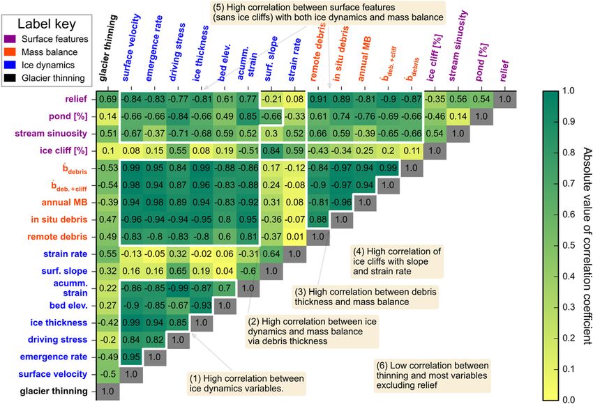
Anderson et al.                                                                                                                        Causes Debris-Covered Glacier Thinning

                                              Keywords: ice cliff, stream, pond, feedback, velocity, expansion, bed, inversion

INTRODUCTION                                                                                    In order to study the complex interactions occurring on
                                                                                            Kennicott Glacier, we attempt to establish causal relationships
Debris cover thicker than a few centimeters insulates the ice                               between various parts of the system, namely debris thickness,
surface beneath it and reduces melt (Østrem, 1959; Nicholson                                melt hotspots, and ice dynamics. Because debris thickness
and Benn, 2006). On debris-covered glaciers, the insulating                                 strongly controls melt, an understanding of the processes
effect of debris appears to strongly control area-averaged melt                             controlling debris thickness is essential for projecting the
rates (Bisset et al., 2020). However, the low melt rates within                             future evolution of debris covered glaciers (e.g., Banerjee,
debris-covered surfaces seem to conflict with the common                                     2017). Processes that control the distribution of sediment on
observation that glacier-wide thinning is often highest                                     glaciers include the melt out of debris from within the glacier, the
beneath melt reducing debris (e.g., Kääb et al., 2012;                                      compression (or extension) of ice due to the pattern of ice
Gardelle et al., 2013). This phenomenon has been referred                                   velocity, the advection of typically thinner debris downglacier,
to as the ‘debris-cover anomaly’ (Pellicciotti et al., 2015); it                            and local sediment re-distribution (hillslope) processes (Moore,
appears to occur globally and has been reported in High                                     2018; Huo et al., 2021). Anderson and Anderson (2018) showed
Mountain Asia, the European Alps (Mölg et al., 2019), and                                   that thin debris should be expected to occur where velocities are
Alaska (Anderson et al., 2021).                                                             high and thick debris should occur where velocities are low. They
    We approach this topic hoping that the study of a single glacier                        suggested that debris melt out from the glacier to the surface
in detail will effectively reveal the underlying processes that                             should decline downglacier following the reduction of melt rates
control the debris cover anomaly more generally. For this case                              under thicker and thicker debris.
study we consider Kennicott Glacier, a large, dynamic glacier in                                Melt hotspots like ice cliffs, streams, and ponds are scattered
the Wrangell Mountains of Alaska (Figure 1).                                                across debris-covered ice surfaces and locally increase melt rates
    To discern the fundamental controls on debris-covered glacier                           (e.g., Miles et al., 2018; Buri et al., 2021). It has been previously
evolution in response to climate change we parse the issue in two:                          shown that ice cliffs correlate with the degree to which surface
First, we consider a modern “snapshot” of Kennicott Glacier                                 flow is compressive (Benn et al., 2012; Kraaijenbrink et al., 2016).
(i.e., frozen in time) to develop our understanding of causal                               Streams on debris-covered glaciers tend to be larger where debris
relationships between different parts of the system. Second, we                             is thin and melt rates are high and smaller where debris is thick
consider the glacier’s evolution over multiple decades.                                     and melt rates are low (Iwata et al., 1980; Fyffe et al., 2019). Ponds

  FIGURE 1 | Context and thinning maps of the study area. (A) Map of Alaska showing the location of panel B as a white square. (B) Kennicott Glacier with the extent
  of panel C as a black rectangle. The contour interval is 200 m. The most southerly contour on the glacier represents 600 m a.s.l. (C) The study area with the rate of glacier
  surface elevation change (dH dt−1) between 1957 and 2004 (see Das et al., 2014). ZMT refers to the zone of maximum thinning and its extent is designated by the double
  headed arrow and the blue dashed lines on the glacier. The solid black line is the trace of the 1,000 m wide swath profile used to present data with distance from the
  terminus in later figures.

Frontiers in Earth Science | www.frontiersin.org                                        2                                              August 2021 | Volume 9 | Article 680995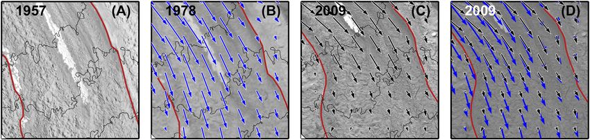
Anderson et al.                                                                                                     Causes Debris-Covered Glacier Thinning

on debris-covered glaciers occur preferentially where surfaces                    velocity in the y-direction. The first term on the right-hand side of
slopes are low (e.g., Reynolds, 2000).                                            Eq. 3 is the rate of debris melt out, the second and third terms
   Previous work has revealed a striking pattern in ice cliffs and                represent the combined effects of surface compression
debris thickness across the debris-covered tongue of Kennicott                    (i.e., surface strain rate, zu/zx+zv/zy) and the advection of
Glacier (Anderson et al., 2021). Where ice cliffs on the modern                   debris in the x- and y-directions.
glacier are most abundant, a rapid increase in debris thickness                       Feedbacks within the debris-covered glacier system are
downglacier also occurs, suggesting that there is a common                        abundant and are represented by the shared terms within and
control. Here we therefore first consider: What controls the                       between Eqs 1–3. Feedbacks occur when a ‘cause’ influences the
patterns of ice flow, debris, and melt hotspots on the modern                      resulting ‘effect’ and the resulting effect loops back to influence
Kennicott Glacier (independent of significant glacier thinning)?                   the cause. As an example, thinning, due to rising temperatures,
To address this question, we produce and compile 18 different                     reduces ice flow causing melt hotspot patterns to change, which in
variables from the modern debris-covered tongue of Kennicott                      turn affects melt rates and thinning, completing the feedback loop
Glacier and cross-correlate them and attempt to establish causal                  (Supplementary Figure S1). Feedbacks are positive when the
relationships by identifying processes that connect the correlated                effect amplifies the cause and negative when the effect lessens
variables.                                                                        the cause.
   When considering the evolution of Kennicott Glacier over                           The chain of process-links from boundary conditions to
several decades, our focus is on explaining how the glacier has                   observables on debris-covered glacier surfaces (like thinning or
thinned and why melt rates appear to have declined in time. The                   ice cliff patterns) are difficult to discern because of the sheer
thinning of glaciers must occur either by mass loss in place or by                number of possible controls. To address and simplify this issue we
dynamical redistribution of mass loss occurring elsewhere on the                  consider: What processes and feedbacks control the thinning of
glacier surface. To show the potential for feedbacks in the debris-               Kennicott Glacier as it thins over multiple decades?
covered glacier system, we highlight three fundamental equations                      We quantified most terms in the first three equations as they
governing the evolution of debris-covered glaciers. First, the                    vary in space and time. All terms of the continuity equation for ice
continuity equation for ice:                                                      (Eq. 1) are quantified, including annual mass balance and ice
                                                                                  emergence. To constrain the glacier thinning pattern we
                           dH _ zuH zvH
                              b−    −    ,                            (1)        difference digital elevation models (DEMs). We quantify all
                           dt     zx   zy                                         terms in the debris–thickness melt relationship (Eq. 2) and the
where H is ice thickness, t is time, b_ is annual area-average mass               continuity equation for debris (Eq. 3) excluding the debris
balance (or loosely ablation in the ablation zone), u is depth-                   porosity and density. The development and inversion for this
averaged velocity in the x-direction, and v is depth-averaged                     range of datasets affords us a rare view into the controls of the
velocity in the y-direction, x-represents east-west direction, and                multi-decadal-scale evolution of a large, rapidly thinning debris-
y-represents the north-south direction. Note that uH and vH are                   covered glacier. Analyses of debris and melt hotspots as they
the ice discharges (Q) in the x- and y-direction, respectively. The               change in time further show how essential ice dynamics are for
last two terms on the right combine to represent ice emergence                    understanding and predicting the evolution of debris-covered
velocity (or surface uplift) and represent the effect of ice dynamics             glaciers.
on glacier thinning. Within the debris-covered zone, mass
balance b_ is the area-averaged melt from beneath debris                          Study Glacier
(b_debris ) and from melt hotspots (b_hotspots ).                                 Kennicott Glacier is 42 km long and broadly faces south-
    Debris thickness affects the melt rate beneath debris through                 southeast in the Wrangell Mountains of Alaska (Figure 1;
Østrem’s curve, which can be described as a hyperbolic                            387 km2 area). As of 2015, 20% of Kennicott Glacier was
relationship [i.e., the Hyper-fit model of Anderson and                            debris-covered (Anderson et al., 2021). Below the equilibrium-
Anderson (2016)]:                                                                 line altitude at about 1,500 m (Armstrong et al., 2017), nine
                                                                                  medial moraines can be identified on the glacier surface. Debris
                                                  hp
                          b_debris  b_ice                   ,         (2)        thicknesses were measured on the glacier surface in 2011 and
                                             (hdebris + hp )                      extrapolated across the central five medial moraines of Kennicott
                                                                                  Glacier (Anderson et al., 2021). Debris thicknesses have also been
where b_ice , is bare-ice melt rate, hdebris is debris thickness, and h* is
                                                                                  estimated across the glacier based on remotely sensed data and
the characteristic debris thickness.
                                                                                  modeling (Rounce et al., 2021). Above 700 m elevation debris is
   Surface debris patterns depend on ice flow and debris
                                                                                  typically less than 5 cm thick, although, near the glacier margin
thickness itself. The governing equation for the evolution of
                                                                                  debris tends to be thicker. Medial moraines coalesce 7 km from
debris thickness (e.g., Nakawo et al., 1986) is
                                                                                  the terminus to form a debris mantle with ice cliffs, streams, and
                  zhdebris      Cb_       zuhdebris zvhdebris                     ponds scattered within an otherwise continuous debris cover. Ice
                                       −          −                   (3)        cliffs are especially abundant on Kennicott Glacier (Anderson
                    zt       1 − ϕρ r     zx        zy
                                                                                  et al., 2021). The zone of maximum thinning, or the ZMT, is
where C is near-surface englacial debris concentration, φ is the                  defined as the portion of the glacier that has thinned at a rate
porosity of the debris, ρr is the density of the rock composing the               greater than 1.2 m yr−1 between 1957 and 2004 (Das et al., 2014;
debris, and u is surface velocity in the x-direction and v is surface             Figure 1). The ZMT has been continuously debris covered since

Frontiers in Earth Science | www.frontiersin.org                              3                                    August 2021 | Volume 9 | Article 680995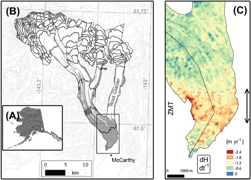
Anderson et al.                                                                                                    Causes Debris-Covered Glacier Thinning

at least 1957 and debris expanded upglacier by 1.6 km between                 Ice Dynamics Terms
1957 and 2009.                                                                Ice Thickness
    Kennicott Glacier has been the focus of outburst flood research            Ice thickness is a fundamental control on the flow of glaciers but
for almost two decades. Each year the ice-marginal Hidden Creek               can be difficult to constrain through debris cover (Pritchard et al.,
lake drains under Kennicott Glacier increasing basal water                    2020). To estimate ice thicknesses along the centerline, we
pressures leading to a 1–2 days period of enhanced basal                      inverted the measured early spring 2013 surface velocities
sliding (Rickman and Rosenkrans, 1997; Anderson et al., 2005;                 from Armstrong et al. (2016) for ice thickness. Ice thickness
Walder et al., 2006; Bartholomaus et al., 2008; Armstrong and                 estimates from previously published, global-scale products have
Anderson, 2020). Armstrong et al. (2016) and Armstrong et al.                 unrealistic step changes in the upper portion of the study area
(2017) showed that up to half of the surface displacement in the              (Farinotti et al., 2019; Supplementary Figures S6–S8). It is a
debris-covered tongue of Kennicott Glacier occurs in the                      common glaciological practice to assume that early spring and
summer, due to sliding at the glacier bed.                                    winter surface velocities result solely from internal deformation
                                                                              (e.g., Armstrong et al., 2016). We acknowledge that winter sliding
                                                                              occurs (e.g., Raymond, 1971; Amundson et al., 2006; Armstrong
METHODS                                                                       et al., 2016), but its magnitude cannot be quantified without
                                                                              borehole observations or independent knowledge of the ice
The data we produced fit into four categories: 1) glacier thinning;            thickness distribution.
2) ice dynamics; 3) mass balance (MB); and 4) surface features                    We used Glen’s flow law to estimate ice thickness H by
(melt hotspots and topography). All data sets were derived from               assuming the flow law exponent n is equal to 3 and solving:
remotely sensed data, except for the in situ measurement of the
                                                                                                                                        1

                                                                                                                   2V′
                                                                                                                                          4
maximum height of 60 ice cliffs during the summer of 2011 (see                                          ⎢                          ⎤⎥⎥⎦
Anderson et al., 2021).                                                                            Hj  ⎡
                                                                                                        ⎢
                                                                                                        ⎣                        3                    (4)
                                                                                                            ASf ρice g sin αj
    We focus on the lower 8.5 km of Kennicott Glacier (Figure 1;
Supplementary Figures S2–S4). Most of the datasets presented                  in which j is the index down the glacier centerline, V′ is the surface
here are based on a 1 km wide swath profile running down the                   velocity vector, with the magnitude of the vector indicated by
center of the glacier. Estimates of annual mass balance and ice               double lines, A is the rate factor, Sf is the shapefactor, ρice is ice
emergence rate represent averages across the glacier surface. Our             density, assumed to be 920 kg m−3, g is the acceleration due to
analysis of the modern glacier surface is based on datasets                   gravity, 9.81 m s−2, and α is the surface slope. We want to solve for
collected between 2011 and 2016. Although these datasets are                  H in Eq. 4, but both Sf and A are unknown, yet they have the same
not all from the same year, we assume that changes in the                     effect on H. By keeping the recommended value of A for
properties are negligible over this period. For temporal                      temperate ice, 2.4 × 10⁻²⁴ Pa−3s−1 (Cuffey and Paterson, 2010)
changes over several decades, we assemble data obtained                       and using a root-mean-squared error (RMSE) metric, we found
between 1957 and 2016.                                                        that a shapefactor of 0.9 best reproduced known ice thicknesses
    We transition between spatial scales, from ‘area-averaged’ to             upglacier from the study area (Supplementary Figure S6). Ice
‘local’ processes. We define ‘area-averaged’ mass balance, as the              thickness near the glacier center is 730 m 12 km upglacier from
mean mass balance over the spatial scale for which the surface                the terminus (Armstrong et al., 2016) and 600 m 10 km up glacier
slope and ice thickness influence ice dynamics, roughly four times             from the terminus (personal communication, Martin Truffer).
the local ice thickness (Kamb and Echelmeyer, 1986). We define                 We assumed that Sf is uniform through the lower 12 km of the
‘local’ as the 1–10 m spatial scale that is relevant for the control of       glacier allowing for the estimation of centerline thickness in the
glacier surface topography by differential ablation.                          swath profile. Uncertainty in ice thickness is estimated by varying
                                                                              the tuned shapefactor (±10%).
Glacier Surface Lowering From 1957 to 2016
To constrain the thinning pattern and its changes in time we
differenced seven digital elevation models (DEMs) covering the                Surface Velocities
period between 1957 and 2016 (Supplementary Table S1 and                      We estimated horizontal glacier surface velocity in 1991, 2005,
Supplementary Figure S5). Before differencing each pair of                    and 2015 using Landsat 5 TM (L5) and Landsat 8 OLI (L8)
DEMs they were co-registered relative to one another using                    imagery (available at earthexplorer.usgs.gov; Supplementary
the pc_align routine in the Ames StereoPipeline software                      Table S3; Supplementary Figure S9). Glacier motion between
(Shean et al., 2016). This was accomplished using the iterative               images taken at different times offsets distinctive pixel “chunks”,
point-to-point algorithm and allowing for the translation of one              with the offset proportional to glacier speed. We utilized Fourier-
raster relative to another with the glacier area masked out.                  space feature tracking implemented in COSI-Corr (Leprince et al.
Uncertainties are based on the standard deviation of elevation                , 2007) to quantitatively estimate feature offsets across Kennicott
change within common, low-sloped areas adjacent to the glacier                Glacier and characterize the spatial distribution of glacier surface
terminus. To minimize seasonal bias, we only differenced DEMs                 velocity. We produced high quality annual velocity estimates
that 1) have acquisition years more than 9 years apart or 2) were             ingesting snow and cloud-free single image pairs from the same
acquired with a day-of-the-year difference of less than 3 weeks               worldwide reference system (WRS) path and row, with input
(Supplementary Table S2).                                                     images spaced approximately 1 year apart. Utilizing input

Frontiers in Earth Science | www.frontiersin.org                          4                                        August 2021 | Volume 9 | Article 680995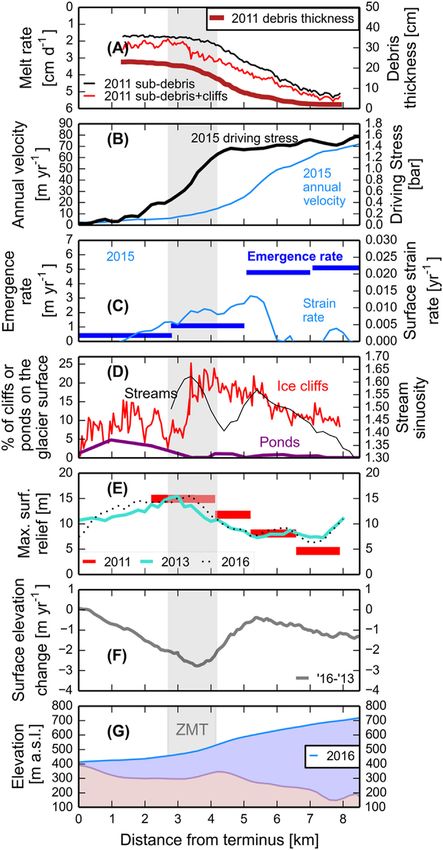
Anderson et al.                                                                                                     Causes Debris-Covered Glacier Thinning

imagery separated by approximately 1 year minimizes seasonal                where this term is positive debris will tend to thicken due to
effects on the velocity pattern that can arise from compositing             compressive flow and where this term is negative, debris will thin
short-term velocity estimates. Despite this long temporal                   due to extensive flow (Supplementary Figure S12). Strain rates
baseline, the feature tracking algorithm still produced high                are calculated across a 200 m × 200 m grid, similar patterns
confidence matches, indicating that the planview appearance                  resulted from calculations based on 400 × 400 m grids. We
of the glacier surface does not change substantially over this              also calculated the amount of strain a debris parcel would
timespan.                                                                   experience as it advected downglacier using the 2015
    We created our own velocity estimates rather than using                 velocity field.
existing velocity products like GO_LIVE (Fahnestock et al.,
2016; Scambos et al., 2016) or ITS_LIVE (Gardner et al., 2018,              Ice Emergence Rates
Gardner et al., 2020) because site-specific tuning of processing             The reduction of ice emergence rates in time can be a strong
parameters and input imagery produces higher quality results for            control on debris-covered glacier thinning (e.g., Vincent et al.,
our single site than these datasets, which are optimized for large-         2016). To estimate ice emergence rates through the study area we
scale applications. The earlier L5 satellite does not have a                used a mass-continuity approach following Bisset et al. (2020).
panchromatic band, so we utilize reflectance in the green                    We divided the glacier surface with across-flow segments
wavelengths (L5 Band 2, 0.52–0.60 μm; L8 Band 3,                            approximately 2 km apart based on glacier outlines derived
0.64–0.67 μm). Reflectance in this waveband has 30 m                         from thinning maps and aerial and satellite imagery. For the
resolution for both L5 and L8 and minimizes potential bias                  2015 ice extent we used the 2009 WorldView (WV) satellite
arising from varying spatial resolution between the missions                image, and a Landsat image from 2016 (Supplementary Figure
(Dehecq et al., 2019). All feature tracking used a step between             S2). For the 1991 ice extent we used a conservative extent based
adjacent estimates of 4 pixels and a variable search window that            on a 1978 USGS aerial photo (a 2004 ice extent produces similar
starts as 64 × 64 pixels, then decreasing to 32 × 32 pixels. The            results; Supplementary Figures S3–S4). Ice emergence rates were
resulting velocity estimates have a spatial resolution of 120 m (4 ×        estimated first by calculating the ice discharge Q:
30 m). Pixels with a signal-to-noise ratio of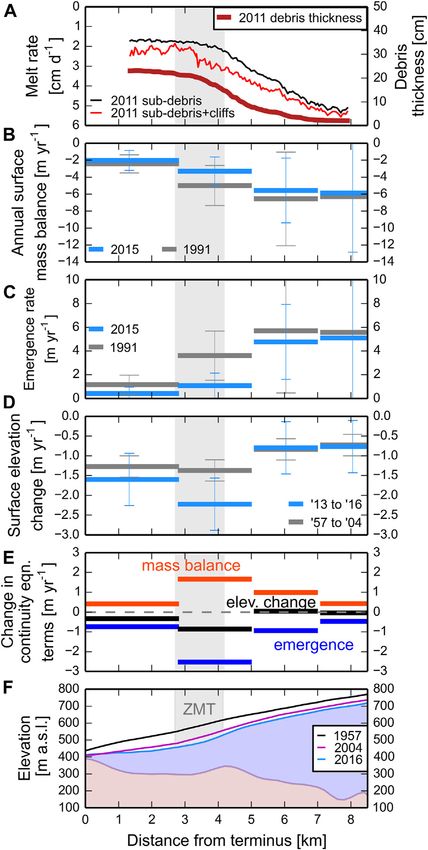
Anderson et al.                                                                                                                  Causes Debris-Covered Glacier Thinning

  FIGURE 2 | Modern snapshot comparison. The zone of maximum
  thinning (ZMT) is shown with grey shading. (A) Surface melt rate and debris
                                                                                          FIGURE 3 | Changes in ice continuity equation terms over multiple
  thickness patterns from the summer of 2011 (Anderson et al., 2021). (B) 2015
                                                                                          decades. The zone of maximum thinning (ZMT) is shown with grey shading.
  annual surface velocity pattern with the driving stress based on the
                                                                                          (A) Debris thickness with distance from the terminus for the 5 central medial
  surface slope and ice thickness from 2016. (C) The ice emergence rate
                                                                                          moraines (Anderson et al., 2021). Distributed melt rate estimates from
  averaged over approximately 2 km intervals as well as the surface strain rate
                                                                                          Anderson et al. (2021). (B) Annual surface mass balance based on 2015
  from the swath profile, smoothed with a 1 km moving window. (D) Patterns of
                                                                                          annual velocities and thinning between 2013 and 2016. As well as the annual
  melt hotspots, including ice cliffs and stream sinuosity from the swath profile,
                                                                                          surface mass balance based on 1991 annual velocities and thinning between
  as well as ponds across the glacier width. (E) Maximum surface relief within
                                                                                          1957 and 2004. (C) The change in ice emergence rate in time. (D) Glacier
  the swath profile taken from 2013 (turquoise) and 2016 (black dots) DEMs.
                                                                                          surface elevation change from 1957 to 2004 and from 2013 to 2016. (E) The
  Maximum measured ice cliff relief (red) from the glacier surface in 2011 is also
                                                                                          change in the terms of the continuity equation between 1991 and 2015. The
  shown. (F) The surface elevation change pattern based on fall 2013 and fall
                                                                                          bars represent the difference between the bars in each of panels B, C, and D.
  2016 DEMs. (G) Glacier surface elevation and bed topography from 2016
                                                                                          (F) Surface profiles through time and the bed profile of Kennicott Glacier.
  down the glacier centerline.

where b_j is the area-averaged mass balance in the glacier                               in which there is a 99.8% probability (±3 standard deviation
section, dH dt−1 is the mean ice surface elevation change. We                            window) that the mass balance estimate lies within the error
followed the error estimation approach of Bisset et al. (2020)                           envelope. These area-averaged mass balance estimates

Frontiers in Earth Science | www.frontiersin.org                                     6                                           August 2021 | Volume 9 | Article 680995
Anderson et al.                                                                                                     Causes Debris-Covered Glacier Thinning

include the contribution of surface, englacial, and sub-                          MacKevett, 1972; MacKevett and Smith, 1972; Miles et al., 2021).
glacial melt.                                                                     Because we have no a priori knowledge of the pattern or
    We produced two estimates of annual mass balance representing                 magnitude of C, porosity, and rock density we ran 13
the years 2015 and 1991. In both cases ice thicknesses were updated               additional inversions in which 1) C increases downglacier
based on the thinning estimates over the intervening timespan. For                linearly through the swath profile by factors of 2, 10, 100, and
the 2015 estimates we used the 2015 velocities as well as thinning                1,000; 2) C decreases linearly downglacier through the swath
data based on fall 2013 and fall 2016 DEMs. For the 1991 mass                     profile by factors of 0.5, 0.1, 0.01, and 0.001; 3) porosity varies
balance estimates, we used the 1991 annual surface velocity as well               between 0.1 and 0.4; 4) rock density varies between 2000 and
as the thinning data based on 1957 and 2004 DEMs. We note that                    2,700 kg m−3; and 5) use the remotely sensed debris pattern of
this long-time interval is not ideal for estimating the mass balance              Rounce et al. (2021) instead of the in situ debris thicknesses as the
in 1991, using annual velocities from 1991. We therefore provide                  2011 evaluating dataset (Supplementary Table S5). The range of
sensitivity analyses to help reveal uncertainties.                                increase in near-surface C downglacier explored (up to 3 orders of
    Additional estimates of mass balance and emergence rate are                   magnitude) is comparable to the increase documented
provided in which we 1) assumed that all ice motion is due to                     downglacier on Khumbu Glacier (Miles et al., 2021).
internal deformation; 2) varied the tuned shapefactor; 3) assumed                    After we used Eq. 10 to calculate 2011 debris thickness
there is no change in thinning rate in time; 4) applied a 2004                    patterns for each of the 1991 debris pattern guesses and value
glacier outline for the 1991 estimates; and 5) applied ITS_LIVE                   of C, we evaluated the calculated 2011 debris thickness patterns
composite velocities (Supplementary Figures S13–S18). Note                        against the measured in situ debris pattern from 2011 using the
that in Figures 2, 3 surface melt rate and debris thickness                       RMSE. A single best 1991 debris thickness pattern and englacial
estimates of Anderson et al. (2021) from the summer of 2011                       debris concentration was identified for each of the 14 inversions.
are plotted for comparison.                                                       Because the contributions of englacial melt out and ice dynamics
                                                                                  were also calculated while solving Eq. 10 we were also able to
                                                                                  explore the role of each in controlling debris thickness change
Inversion to Estimate Debris Thickness                                            in time.
Change and Englacial Debris Concentration
To aid in our understanding of the evolution of Kennicott Glacier                 Melt Hotspots and Surface Relief
in time we estimated debris thickness changes between 1991 and                    Melt hotspots are associated with surface features like ice cliffs,
2011 as well as the mean englacial debris concentration in the                    surface streams, and surface ponds which locally enhance melt
study area. To do this we inverted measured debris thickness,                     and thinning. We used the delineated ice cliff extents from
surface velocities, strain rates, and annual mass balance estimates               Anderson et al. (2021), who used an Adaptive Binary
from the swath profile.                                                            Threshold method applied to a 0.5 m resolution WV satellite
    The first step used a Monte Carlo approach to estimate 106                     image (from July 13, 2009; Supplementary Table S4).
potential 1991 debris thickness patterns (e.g., Tarantola, 2005).
We allow random changes in each 200 m pixel from the 2011 in                      Supraglacial Streams
situ debris thickness pattern to generate possible 1991 debris                    Streams paths on the glacier surface were delineated using the
thickness patterns. Second, for each possible 1991 debris                         GRASS GIS command r.stream.extract and a fall 2013 DEM with
thickness pattern and englacial debris concentration we                           a 2 m spatial resolution (Porter et al., 2018; Supplementary Table
numerically solved Eq. 3 in this form starting in 1991 until an                   S1). Because of the complex topography on the glacier surface,
estimate of 2011 debris thickness was produced:                                   and observations of many undercut streams the filling of
                                                                                  depressions less than 16 m2 was required to produce viable
                Cb_ (x)                        zhdebris (x)
   zhdebris            − ε_ (x)hdebris (x) −                V′ (x)dt         stream paths on the glacier surface. Stream sinuosity S was
               1 − ϕρr                           zx
                                                                                  then calculated along individual stream paths using
                                                                       (10)       TopoToolbox 2 (Schwanghart and Scherler, 2014) and the
The first term on the right is the contribution of englacial debris                equation:
melt out, the second term is the contribution of compression or                                                    Lchannel
extension, and the third term represents the advection of debris                                              S                                      (11)
                                                                                                                   Lstraight
downglacier. The timestep, dt is set to 1 year hdebris is initially
h1991
 debris and is then updated in each timestep as the debris thickness
                                                                                  where Lchannel is the length of the channel and Lstraight is the
evolves. For b_ we used linearly interpolated annual mass  balances

                                                                                  straight-line distance downstream. An S value of 1 represents a
for each year between the 1991 and 2015 estimates. For V′  (_ε) we            straight stream. The higher the value of S the more sinuous the
used linearly interpolated surface velocities (strain rates) for each             stream. Each sinuosity value was calculated over a reach of 400 m.
year between the 1991 and 2015 following the rate of change                       Uncertainties in surface stream sinuosity are estimated by varying
through time shown in Supplementary Figure S9.                                    the 400 m reach by ±100 m. Because sinuosity values at either end
   For the case presented in the main text we assumed that C is                   of a stream segment are biased due to the lack of a downstream
uniform and does not vary in time, that porosity is 0.3 (Nicholson                reach, stream sinuosities were not plotted or analyzed for the
and Benn, 2013), and that the rock density is 2,200 kg m−3 (see                   upper and lower 200 m of each stream. Streams at the glacier

Frontiers in Earth Science | www.frontiersin.org                              7                                     August 2021 | Volume 9 | Article 680995
Anderson et al.                                                                                                  Causes Debris-Covered Glacier Thinning

margin were removed from the sinuosity calculations. In order to               the bed topography is predicted just upstream from the zone of
identify where streams are present at the glacier margin, we                   maximum thinning (ZMT) under the surface topographic bulge
digitized their paths in QGIS using the 2009 WV image.                         (at ∼4 km in Figure 2G). Upglacier from the ridge, the bed is
                                                                               overdeepened (bed elevations are lower upglacier). The lowest
Supraglacial Ponds                                                             bed elevation predicted within the study area is 150 m a.sl., 7.7 km
Pond coverage was determined for two time periods. Pond extent                 upglacier from the terminus, where the glacier is estimated to be
was hand digitized from a United States Geological Survey                      550 m thick. A 10% change in the tuned shapefactor results in a
(USGS) 1957 aerial photo and the 2009 WV image in QGIS.                        10% change in bed elevation.
Ponds were searched for using a fixed grid to ensure complete                      Independent of the period examined, glacier thinning is
coverage of the study area. Depressions on the glacier surface with            highest in the ZMT (Figure 3D and Supplementary Figure
exposed ice and/or ice-cut shorelines were digitized and assumed               S5). Surface lowering rates increased towards the present.
to be drained ponds.                                                           Between 1957 and 2004 the surface lowering rate was
                                                                               −1.4 m yr−1 within the ZMT and between fall 2013 and fall
Glacier Surface Relief                                                         2016 the surface lowering rate was −2.2 m yr−1. Uncertainties
The topography of debris-covered glacier surfaces can vary widely              for surface lowering rates used in the main text range from ±0.66
over ten- to hundred-meter scales (Iwata et al., 1980). Relief is the          to 0.27 m yr−1 (Supplementary Table S2).
difference in elevation between the highest and lowest point within a
given area. In order to assess how finer scale topography has changed           Ice Dynamics Terms
through time on Kennicott Glacier we estimated glacier surface relief          Surface velocities decrease downglacier and towards the glacier
at 50 m resolution using the Raster Terrain Analysis Plugin in QGIS            margin. For the 2015 (1991) surface velocities, maximum annual
for three DEMs. We measured maximum surface relief within each                 surface velocities of 75 (105) m yr−1 occur in the upper portion of
band of the swath profile for the 1957 (shown in the Supplementary              the study area (Figure 4B and Supplementary Figure S9). The
Figures), as well as the fall 2013 and fall 2016 DEMs. Uncertainties in        2015 (1991) surface velocities become indistinguishable from
the DEMs are presented in Supplementary Table S1. Because the                  noise 3 (1.8) km upglacier from the terminus.
1957 USGS DEM has an original resolution of 60 × 30 m we chose an                 The terminal region of Kennicott Glacier slowed substantially
intermediate resolution of 50 m over which to calculate glacier surface        over the study period, with a ∼40 m yr−1 (∼50%) velocity decrease
relief.                                                                        between 1991 and 2015 (Supplementary Figure S9). Most of the
    We also measured maximum relief of 60 ice cliffs in the summer of          velocity change occurred between 1991 and 2005, with only
2011 using a laser rangefinder (see Anderson et al., 2021 for locations).       minor slowing occurring after this time. The fact that most of
Uncertainty in these estimates arises from not targeting the actual            the slowing occurred between the early and middle time periods,
location of lowest elevation at the base of the ice cliff. To reduce           which are both estimated using L5 imagery, indicates that this is
uncertainty five measurements were taken from possible lowest points            not an artifact of intermission comparison, radiometric range,
at each ice cliff and the maximum value is reported. Error in these            and spatial resolution of the sensors (Dehecq et al., 2019). Our use
estimates is unlikely to exceed 1 m.                                           of a fixed spatial resolution for input images, restriction to snow-
                                                                               free acquisitions, and the study area being in a wide and low
Correlation Between Variables                                                  elevation location minimizes potential biases. For L5, velocity
To guide the analysis relating ice dynamics, debris, and melt hotspots         uncertainty is on the order of 10–15 m yr−1, while it is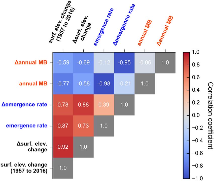
Anderson et al.                                                                                                                 Causes Debris-Covered Glacier Thinning

  FIGURE 4 | Changes in debris extent. Each panel reflects the same 3 × 3 km area on the glacier surface (see Figure 6). Red lines in each panel represent the border
  between the same medial moraines. Note the distinct change in medial moraine boundaries through time, especially between 1978 and 2009. (A) 1957 aerial photo. (B)
  1978 aerial photo with annual surface velocity vectors from 1991. The largest vector at the top of the panel has a magnitude of 105 m yr−1. (C) 2009 WorldView image
  with annual surface velocity vectors from 2015. The largest vector at the top of the panel has a magnitude of 75 m yr−1. Flow is compressive where debris extent
  has expanded. (D) 2009 WorldView image, with darker shade, overlaid with annual surface velocity vectors from 2015, in black with white outlines, and the annual
  surface velocity vectors from 1991 in blue.

2C, 3C). Ice emergence rates declined throughout the study area
from 1991 to 2015, most within the ZMT (2.4 m yr−1) and
within 2 km upglacier of the ZMT (1.95 m yr−1). Ice
emergence rates changed least below the ZMT and at the
upglacier end of the study area. Uncertainties (±3 St. dev.)
scale with the magnitude of the emergence rate and range from 1
to 9 m yr−1. While there are significant uncertainties in the
estimates of ice emergence rate, ice emergence rate is the
dominant control on thinning in the ZMT for all sensitivity
tests (Supplementary Figures S13–S18).

Annual Mass Balance
Annual surface mass balance appears to have increased from 1991
to 2015, suggesting that melt rates decreased towards the present
in the study area (Figures 3B,E). The largest estimated reduction
in annual melt rates occurred in the ZMT (+2.1 m yr−1) and in an
area of the glacier just upglacier from the ZMT (+1.8 m yr−1).
While there are significant uncertainties in the estimates of
annual mass balance, the reduction in melt rate between 1991
and 2015 is present in all sensitivity tests (Supplementary
Figures S13–S18).

Inversion to Estimate Debris Thickness
Change and Englacial Debris Concentration
Figure 5 shows an estimate of how debris thickness changed in
time in the study area assuming uniform englacial debris
concentrations. Panels B and C show the change in debris
thickness from 1991 to 2011. Panels B and C also show the                                FIGURE 5 | The debris feedback expressed on the surface of Kennicott
absolute and relative roles of ice dynamics and debris melt out in                       Glacier. For all panels the zone of maximum thinning (ZMT) is shown in grey.
                                                                                         (A) Annual surface velocities from 1991 to 2015 from the swath profile. (B) In
changing debris thickness. In all 14 inversions, debris melt out
                                                                                         situ debris thickness from 2011. The best estimate of the debris pattern
occurs across the study area and decreases downglacier. This                             in 1991 is shown as well as the simulated debris thicknesses in 2011
occurs because ice is melting across the study area and area-                            produced from the inversion assuming a uniform englacial debris
averaged melt rates decline downglacier. Ice dynamics thickens                           concentration. (C) Predicted absolute change in debris thickness from 1991
debris within and below the ZMT and tends to thin debris above                           to 2011 due to dynamics and debris melt out. (D) The relative role of ice
                                                                                         dynamics and debris melt out in debris thickness change. Above the ZMT
the ZMT. This dynamical effect is present in all inversion                               debris melt out accounts for 100% of the debris thickening because flow is
scenarios and is the result of the measured patterns of surface                          high and ice dynamics tends to thin debris by advection there.
velocity and strain rate.

Frontiers in Earth Science | www.frontiersin.org                                    9                                           August 2021 | Volume 9 | Article 680995
Anderson et al. Causes Debris-Covered Glacier Thinning
FIGURE 6 | Comparison of thinning, melt hotspots, and melt in map view. The double headed arrows indicate the extent of the zone of maximum thinning (ZMT). (A)
Glacier surface elevation change between 1957 and 2004 and observed surface pond extent in 1957 (white) and 2009 (black). The 1957 glacier extent is shown by the
extent of the thinning map. The 2015 glacier outline is shown in black, as is the boundary between the central 5 medial moraines (compare with panel D). (B) Ice cliff
coverage in fractional area ×100 (percent) from Anderson et al. (2021) with a 100 m grid. The black box shows the extent of each panel in Figure 4. (C) Supraglacial
stream extent and sinuosity across the study area. Ice marginal streams digitized from the 2009 WorldView image are shown as yellow lines. The proglacial lake in 2009 is
shown in blue. (D) Sub-debris melt estimates from the summer of 2011 (Anderson et al., 2021). Contours are derived from a 2015 DEM.
The mean of all inversions for the average englacial debris Stream paths are longer above the ZMT than below the ZMT
concentration across the study area was 0.017% by volume with a (Figure 6C). Stream sinuosity is low in the upper portion of the
standard deviation of 0.0076% (Supplementary Table S5). The study area and increases downglacier until the middle of the ZMT
maximum average englacial debris concentration from a single (Figures 2D, 6C). Streams tend to be less sinuous in the upper
inversion run was 0.033% and the minimum was 0.007%. The portion of the study area and become increasingly sinuous until
estimated mean concentrations are comparable with previous the middle of the zone of maximum thinning. Field investigations
near-surface measurements from other glaciers (e.g., Bozhinskiy in the summer of 2011 and digitization of streams on the glacier
et al., 1986; Miles et al., 2021). All 14 inversions for surface debris surface using the WV images suggest that streams are limited on
thickness change between 1991 and 2011 indicated that on the glacier surface below the upper portion of the ZMT
average debris thickened in the study area. Almost all (Supplementary Figure S23). At the transition between these
estimates indicated that debris thickened most in and domains in the middle of the ZMT the largest supraglacial
downglacier from the ZMT (Supplementary Figure S20) streams descend into a series of moulins or flow off glacier
where both dynamics and debris melt out contribute to debris (Anderson, 2014). A 10% change in the distance over which
thickening. sinuosity is calculated changes the mean sinuosity across the
study area by 2.2%.
Surface pond area is largest below the ZMT (Figure 6A and
Melt Hotspots, Surface Slope, and Surface Supplementary Figure S22). Based on the 2009 WV image
Relief ponds are most abundant 1 km upglacier from the terminus
Area-averaged surface slopes declined below the ZMT and tended and occupied about 5% of the glacier surface. Uncertainty in
to increase in the upper portion of the ZMT and 1 km above the 2009 pond area, based on digitization by an independent
ZMT (Supplementary Figure S21). Modern maximum glacier operator, is ±1% of the glacier surface. Digitized 1957 pond
surface relief is highest in the ZMT, remains high downglacier extents show that ponds were largely present near the
towards the terminus and decreases upglacier from the ZMT terminus with a maximum of about 5.5% of the glacier surface
(Figure 2E). The location of maximum glacier surface relief was near the terminus. Uncertainty in 1957 pond area, based on
near the toe in 1957 and shifted into the ZMT towards the present digitization by an independent operator, is ±2% of the glacier
(Supplementary Figure S22). In and above the ZMT maximum surface. Pond coverage increased from 1957 to 2009 (Figures 3D,
relief increased from 1957 to 2016. Uncertainties in the DEMs 6A). Upglacier from the ZMT ponds are only abundant in medial
used to calculate relief range from 15 m for the 1957 DEM to less moraines near the glacier margin, where debris tends to be thicker
than 3 m for the ArcticDEMs (Supplementary Table S1). and ice flow slower than near the glacier center.
Frontiers in Earth Science | www.frontiersin.org 10 August 2021 | Volume 9 | Article 680995Anderson et al. Causes Debris-Covered Glacier Thinning
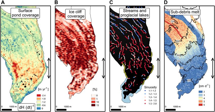
FIGURE 7 | Correlations from the modern snapshot. All datasets are derived from between 2011 and 2016. Correlations between all 18 variables are contained in
this matrix. The green-yellow color bar shows the magnitude of correlation. The sign of correlation can be read from the black labels in each cell. Cells with high magnitude
of correlation are outlined in white and described with annotations on the figure. The numbers in the annotations follow the chain of process links presented in the
discussion. Relief for example can be correlated with all other properties by starting at the upper left and looking across the row to the relief label in the upper right.
Pond (%) can be correlated with all other variables by starting with the upper left label and continuing across the row until the last cell and then looking vertically to see the
correlation between pond (%) and relief. Note that increased thinning is represented by positive numbers in this figure. This contrasts with Figure 8 where more negative
surface elevation change is equivalent to more positive thinning.
Correlation Between Variables terms and in situ debris thickness are all higher than 0.8. The
Figure 7 shows the cross-correlation matrix for the modern cumulative sum of compression is highly correlated with debris
snapshot. Ice dynamics variables show strong correlations with thickness (r 0.95). Debris thickness patterns on Kennicott
one another. Surface velocity and ice thickness are highly Glacier follow the inverse of surface velocity (r −0.94). In
correlated with ice emergence rate (r 0.99 and 0.95). situ debris thickness is highly correlated with all mass balance
Variations in ice thickness are highly correlated with bed estimates (r > 0.96).
elevation (r −0.93) and therefore bed elevation is also The relief of the glacier surface is linked to in situ debris
strongly associated with the other ice dynamics variables. thickness and mass balance (r greater than at least 0.81). Relief
Surface slope and strain rate are generally only weakly is also highly correlated with ice dynamical terms. Relief is the
correlated with other dynamical terms. The surface slope plays variable most highly correlated with glacier thinning (r 0.69).
a role in setting the ice dynamical terms through Glen’s flow law, Ice cliffs correlate highly with surface strain rates and slope (r
but its role is secondary to ice thickness, especially for low sloped 0.59 and 0.84 respectively; Supplementary Figures S19, S21). On
glaciers like the Kennicott. The strain rate is determined by the Kennicott Glacier, 2009 surface ponds are more abundant below
gradient in surface velocity terms and therefore does not correlate the ZMT and are most strongly correlated with driving stress (r
with most other ice dynamics variables, which are more closely −0.84; Supplementary Figure S22) and surface slope (r −0.66).
linked to velocity at a single point. Figure 8 is the cross-correlation matrix for glacier change over
The ice dynamical terms have high magnitudes of correlation multiple decades. See Figure 3 for the signs of individual terms in
with the annual mass balance estimates from 2015 and the Figure 8. Glacier surface elevation change (1957–2016) and its
independent summer 2011 melt rate estimates from Anderson change in time (1957–2004 minus 2013–2016) are both highly
et al. (2021). The magnitude of correlation between ice dynamical positively correlated (red) with the decline in ice emergence rate
Frontiers in Earth Science | www.frontiersin.org 11 August 2021 | Volume 9 | Article 680995Anderson et al. Causes Debris-Covered Glacier Thinning
the ZMT likely exists due to a rise in the glacier bed beneath it.
Because the glacier thins here, it must steepen to pass the same ice
discharge coming from the thick ice upstream. Further
geophysical surveys are needed to confirm this inference.
Surface Velocity Controls Debris Thickness and Mass
Balance
Surface velocity is an important control on debris thickness
patterns (Figure 5). Within and below the zone of maximum
thinning, ice dynamics and debris melt out both tend to thicken
debris. Because surface speeds are low here downglacier
translation of thin debris is also low allowing debris
compression to thicken debris locally. Above the ZMT ice
dynamics tends to thin debris while debris melt out tends to
thicken debris. High surface speeds translate debris downglacier
rapidly (Figure 5). In other words, within a given pixel thin debris
is translated from upglacier leading at an apparent thinning of
debris. This dynamic thinning effect is compensated for by the
rapid melt out of debris from within the glacier (Figure 5C).
FIGURE 8 | Correlations between ice continuity terms as they change We can expect these same general patterns on other debris
over multiple decades. Correlations between all terms in the continuity covered glaciers: where velocities are high debris thicknesses will
equation can be read from the matrix. As an example: A high positive tend to be low, where velocities are low debris thickness will tend to
correlation (red) between surface elevation change and Δemergence rate
indicates that the negative surface elevation change from 1991 to 2015 is
be high. The results from Kennicott Glacier bolster the theoretical
positively correlated with the negative decline in ice emergence rate in time. arguments laid out first by Kirkbride (2000) and later supported
See Figure 3 for the patterns and signs of each term in this figure. and expanded upon by Anderson and Anderson (2018).
The control of surface velocities on debris thickness means
that area-average melt rates are also highly correlated with surface
in time. In other words where thinning was highest the reduction velocity and ice emergence rates. The high correlation between
in emergence rate was also highest and where the change in annual mass balance and ice emergence rate is expected because
thinning was highest the decline in emergence rates in time was they compensate for one another via feedbacks between surface
also highest. In contrast surface elevation change and its change slope and ice thickness as is also the case for glaciers unperturbed
in time are negatively correlated with annual mass balance and its by debris (e.g., Hooke, 1998). The co-evolution of ice dynamics
change in time. This means that where melt is high thinning tends and surface melt is a result of inevitable physical relationships (see
to be low and where thinning has increased in time melt rates Eq. 3) for debris-covered glaciers and should therefore be
have decreased in time. observed generally.
Thin Debris and Dynamic Thinning Control Surface
DISCUSSION Relief
Glacier surface relief correlates highly with most variables in
In the discussion we build a chain of process links evident on the Figure 7. Process controls on relief assuredly vary in space,
modern surface of Kennicott Glacier starting from the glacier bed. depending on location relative to the ZMT and whether flow
We use the correlation coefficients presented in Correlation is rapid or slow. Where flow is high, surface roughness is linked to
Between Variables and Figure 7 to help identify processes area-averaged debris thickness as differences in local melt rate
links for the modern snapshot. Next, we delve into how these help produce surface topography (e.g., Anderson, 2000; Moore,
process links change over several decades including feedbacks 2018). Because of the hyperbolic shape of Østrem’s curve, where
related to changes in the terms of Eq. 1 in Processes Controlling area-averaged debris thicknesses are low, small differences in
Glacier Change Over Multiple Decades. debris thickness produce large differences in local melt rate that
rapidly increase local surface relief. The glacier surface acts like a
conveyor belt, so it follows that relief cumulatively increases
Chain of Process Links From the Modern downglacier above the ZMT. The further down glacier the
Snapshot longer differential melt has acted to increase local relief.
Expression of the Glacier Bed in Surface Velocity Streams are expected to increase relief production above the
The bed pattern explains the pattern of ice dynamics apparent ZMT as discussed in Ice Cliff-Stream-Relief Feedback.
across the study area. Based on Glen’s flow law, glacier surface Below the ZMT, where flow is low and debris is generally thick,
velocity varies with ice thickness to the power of 4 and surface small differences in debris thickness do not produce significant
slope to the power of 3 (Equation 4; e.g., Hooke, 1998). The differences in melt rate, limiting relief production. Below the
topographic bulge on the glacier surface near the upglacier end of ZMT, tunnel collapse has an important role in relief production
Frontiers in Earth Science | www.frontiersin.org 12 August 2021 | Volume 9 | Article 680995Anderson et al. Causes Debris-Covered Glacier Thinning
(e.g., Benn et al., 2017). Interestingly, across the study area, glacier Stream Sinuosity Varies With Roughness and Surface Slope
thinning is most highly correlated with surface relief. Because Estimated stream sinuosity increases downglacier with glacier
dynamic glacier thinning directly changes glacier surface surface relief (Figure 2D). At the upper end of the study area
elevations (via the decline in emergence rates in time) it troughs between medial moraines are more linear and stream
follows that surface relief should correlate with thinning. sinuosity is low. As the medial moraines coalesce downglacier the
troughs are occupied by increasingly chaotic topography just as
Debris Thickness and Ice Dynamics Control Melt streams become more sinuous. Supraglacial streams on
Hotspots uncovered glaciers tend to be more sinuous where slopes are
Melt hotspots have distinctive patterns on the surface of steep and water discharge is high (Ferguson, 1973); observations
Kennicott Glacier. A number of processes connect debris and that also appear to apply within the debris cover of Kennicott
ice dynamics with ice cliffs, streams, ponds, and relief which we Glacier. Without further field investigations into the dynamics of
describe below. supraglacial streams, it is hard to discern the degree to which
rough surface topography or the physics of supraglacial stream
Ice Cliffs are Abundant Where Compression and Surface flow itself controls stream sinuosity on debris-covered ice.
Slopes are High
Ice cliffs are most abundant where surface compression is high on Ice Cliff-Stream-Relief Feedback
Kennicott Glacier. A correlation between strain rate and ice cliffs also A positive feedback between ice cliffs, surface streams, and surface
occurs on glaciers in the Himalaya (Benn et al., 2012; Kraaijenbrink relief occurs on Kennicott Glacier. Streams and ice cliffs should
et al., 2016; Supplementary Figure S19). But to date no clear process amplify the occurrence of each other: melt from ice cliffs increases
connecting surface compression and ice cliff coverage has been stream flow and streams maintain ice cliffs by undercutting them.
identified. One way in which surface compression could increase ice Undercutting streams can create gaps between ice cliffs and the
cliff abundance is if debris compression is manifested in a non- debris-covered surface below via thermal erosion (Reid and Brock,
uniform fashion and localized in shear bands. This would lead to the 2010; Supplementary Figure S24). This prevents ice cliff burial
increase of local debris thicknesses in some areas and not others, while still allowing debris, that trundles down the ice cliff, to
therefore allowing for differential melt, local surface slope accumulate across the stream.
steepening, and ice cliff formation. Importantly, stream undercutting is enhanced where streams
An assessment of local patterns of ice emergence rate (surface are more sinuous (Parker, 1975). As a result, the arc-shaped
uplift) is also needed to determine if dynamic steepening and ice meander bends of streams help maintain arc-shaped ice cliffs
cliff abundance correlate. Short-lived high-compression events (Supplementary Figure S24). The arc-shaped ice cliffs focus
may also play a role on Kennicott Glacier. The annual summer trundling debris into a smaller area, locally increasing debris
flood of Hidden Creek Lake produces a period of very rapid sliding thickness and increasing debris thickness variability in space. Via
(e.g., Bartholomaus et al., 2008), translating the entire ice column differential melt, local surface topography will grow in time,
down glacier leading to high strain rates exactly where ice cliffs are which can produce additional ice cliffs and increase stream
abundant. Perhaps the shaking of the glacier surface during the sinuosity by roughening the glacier surface, therefore
summer flood encourages debris failure and cliff formation? completing the positive feedback loop.
Ice cliffs on Kennicott Glacier are positively correlated with It is likely that this feedback will apply on other glaciers where 1)
surface slope (Supplementary Figure S21). Where area-averaged area-average debris is relatively thin (less than 20 cm), so relatively
surface slopes are high debris failure is more likely. Steep debris- high melt rates can increase stream flow and 2) surface strain rates
covered slopes on the glacier surface, present due to differential and slopes are high increasing ice cliff abundance. Sato et al. (2021)
melt, can be steepened even further as they are passively found a correspondence between drainage patterns and ice cliff
transported into areas with steep area-averaged slopes. This occurrence on the more heavily debris covered Trakarding Glacier
steepening effect would tend to encourage ice cliff formation in the Nepalese Himalaya. The thicker the debris the less likely
and persistence. But on Kennicott Glacier area-averaged slopes streams are to undercut ice cliffs precluding the occurrence of this
tend to be low (You can also read