Large-scale changes of the semidiurnal tide along North Atlantic coasts from 1846 to 2018 - OS
←
→
Page content transcription
If your browser does not render page correctly, please read the page content below
Ocean Sci., 17, 17–34, 2021
https://doi.org/10.5194/os-17-17-2021
© Author(s) 2021. This work is distributed under
the Creative Commons Attribution 4.0 License.

Large-scale changes of the semidiurnal tide along North Atlantic
coasts from 1846 to 2018
Lucia Pineau-Guillou1 , Pascal Lazure1 , and Guy Wöppelmann2
1 IFREMER,   CNRS, IRD, UBO, Laboratoire d’Océanographie Physique et Spatiale, UMR 6523, IUEM, Brest, France
2 LIENSS,   Université de la Rochelle-CNRS, La Rochelle, France

Correspondence: Lucia Pineau-Guillou (lucia.pineau.guillou@ifremer.fr)

Received: 29 May 2020 – Discussion started: 15 June 2020
Revised: 5 November 2020 – Accepted: 10 November 2020 – Published: 4 January 2021

Abstract. We investigated the long-term changes of the prin-      1   Introduction
cipal tidal component M2 along North Atlantic coasts, from
1846 to 2018. We analysed 18 tide gauges with time se-            Tides have been changing due to non-astronomical fac-
ries starting no later than 1940. The longest is Brest with       tors since the 19th century (Haigh et al., 2019; Talke and
165 years of observations. We carefully processed the data,       Jay, 2020). In the North Atlantic, secular variations have
particularly to remove the 18.6-year nodal modulation. We         been observed at individual tide gauge stations, e.g. Brest
found that M2 variations are consistent at all the stations in    (Cartwright, 1972; Wöppelmann et al., 2006; Pouvreau et al.,
the North-East Atlantic (Cuxhaven, Delfzijl, Hoek van Hol-        2006; Pouvreau, 2008), Newlyn (Araújo and Pugh, 2008;
land, Newlyn, Brest), whereas some discrepancies appear in        Bradshaw et al., 2016), New York (Talke et al., 2014), and
the North-West Atlantic. The changes started long before the      Boston (Talke et al., 2018), but also at regional scale, e.g.
20th century and are not linear. The secular trends in M2 am-     Gulf of Maine (Doodson, 1924; Godin, 1995; Ray, 2006; Ray
plitude vary from one station to another; most of them are        and Talke, 2019), at the North Atlantic basin scale (Müller,
positive, up to 2.5 mm/yr at Wilmington since 1910. Since         2011), and at a quasi-global scale (Woodworth, 2010; Müller
1990, the trends switch from positive to negative values in the   et al., 2011; Mawdsley et al., 2015). Long-term changes in
North-East Atlantic. Concerning the possible causes of the        tidal constituents are rather small at some coastal stations
observed changes, the similarity between the North Atlantic       but tend to be statistically significant. The order of magni-
Oscillation and M2 variations in the North-East Atlantic sug-     tude of these changes varies spatially and may reach a few
gests a possible influence of the large-scale atmospheric cir-    centimetres per century for M2 amplitude. For example, Ray
culation on the tide. Our statistical analysis confirms large     and Talke (2019) found trends varying from −1 to 8 cm per
correlations at all the stations in the North-East Atlantic. We   century in the Gulf of Maine over the last century. Wood-
discuss a possible underlying mechanism. A different spatial      worth et al. (2010) and Müller et al. (2011) found trends of a
distribution of mean sea level (corresponding to water depth)     few percent per century in the Atlantic. The changes can be
from one year to another, depending on the low-frequency          larger in many estuaries and rivers (Talke and Jay, 2020).
sea-level pressure patterns, could impact the propagation of         The physical causes of these changes can be multiple
the tide in the North Atlantic basin. However, the hypothesis     and difficult to disentangle. In particular, the complexity
is at present unproven.                                           comes from the possible interaction between local and large-
                                                                  scale causes. Changes may have a local-scale origin, such
                                                                  as changes in the nearby environment (e.g. harbour develop-
                                                                  ment, deepening of channels, dredging, siltation) or changes
                                                                  in the instrumentation (e.g. tide gauge technology, observa-
                                                                  tory location, instrumental errors). For example, Familkhalili
                                                                  and Talke (2016) show that mean tidal range at Wilmington
                                                                  has doubled since the 1880s, due to channel deepening in

Published by Copernicus Publications on behalf of the European Geosciences Union.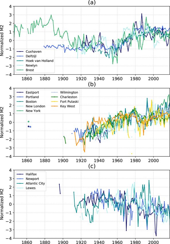
18                                                      L. Pineau-Guillou et al.: Large-scale changes of the semidiurnal tide

the Cape Fear River estuary. Changes may also have a large-        mospheric circulation, already mentioned by Müller et al.
scale origin, i.e. regional or global. Haigh et al. (2019) re-     (2011), on the basis of qualitative criteria. Here, we further
ported several possible large-scale mechanisms: (1) tectonics      provide quantitative insights into the possible influence of the
and continental drift, (2) water depth changes due to mean         NAO and discuss a possible NAO-related climate mechanism
sea level rise or geological processes such as the Earth’s sur-    that can partly explain the observed changes.
face glacial isostatic adjustment (Müller et al., 2011; Pick-         The paper is organized as follows. The first section be-
ering et al., 2017; Schindelegger et al., 2018), (3) shoreline     low describes the data: the sea level data (i.e. tide gauges
position, (4) extent of sea-ice cover (Müller et al., 2014), (5)   and their processing) and the atmospheric data (i.e. climate
sea-bed roughness, (6) ocean stratification which may mod-         indices and sea level pressure data). The following section
ify the internal tides and bottom friction over continental        presents the results (i.e. M2 variations and trends). We then
shelves (Müller, 2012), (7) non-linear interactions, and (8)       discuss a possible link between the observed tidal changes
radiational forcing (Ray, 2009).                                   and MSL, as well as climate indices.
   Several authors have explored mean sea level (MSL) rise
as a potential mechanism to explain M2 changes. For exam-
ple, simulations by Pickering et al. (2012) show that a 2 m        2     Data
sea level rise could modify M2 from −20 to 20 cm around the
                                                                   2.1     Sea level data
whole ocean. Idier et al. (2017) show that depending on the
location, the changes can account for ±15 % of the regional        2.1.1    Tide gauge selection
sea level rise. Schindelegger et al. (2018) find changes of
about 1 %–5 % of the sea level rise. Beyond MSL rise, other        The tide gauge data were retrieved from the University of
mechanisms have been explored to explain M2 changes. For           Hawaii Sea Level Center (UHSLC, website accessed April
example, Colosi and Munk (2006) attribute the changes of           2020). The dataset consists of 249 stations in the Atlantic
M2 amplitude at Honolulu, Hawaii, to a 28◦ rotation of the         Ocean, with hourly sea level observations. Two additional
internal tide vector in response to ocean warming. Ray and         long-term stations – Delfzijl and Hoek van Holland – were
Talke (2019) suggest that long-term changes in stratification      provided by Rijkswaterstaat (RWS) in the Netherlands.
could play a role in the Gulf of Maine. Müller (2011) sug-            We selected the stations following three criteria: time se-
gests a possible link between M2 changes and atmospheric           ries (1) starting before 1940, (2) with at least 80 years of
dynamics in the North Atlantic; he reported that the time se-      data, and (3) with tidal amplitude significant enough to detect
ries of the North Atlantic Oscillation (NAO) show similar          trends, i.e. M2 amplitude larger than 10 cm. Note that we se-
characteristics to those of the tidal amplitudes and phases.       lected only years with at least 75 % of data (see Sect. 2.1.2).
In the Gulf of Maine, Pan et al. (2019) suggest that changes       Only 24 stations among the 249 from UHSLC fulfilled the
in the response of the nodal modulation of the M2 tide from        two first criteria (Fig. 1). They are all located in the Northern
1970s to 2013 may be linked with the NAO. In Southeast             Hemisphere. On the east side of the North Atlantic, Stock-
Asian waters, Devlin et al. (2018) show that the impact of at-     holm, Gedser, Hornbaek, Tregde and Marseille were dis-
mospheric circulation (via the wind stress, through Ekman          carded due to too small of an M2 amplitude (i.e. lower than
current) on the M2 seasonal cycle may be significant and           10 cm). These stations are located in the Baltic Sea (Stock-
comparable to the effect of permanent (geostrophic) currents.      holm, Gedser), in the strait separating the Baltic and the
In the North Sea, Huess and Andersen (2001) explain a large        North Sea (Hornbaek), in the North Sea (Tregde), and in
part of M2 seasonal cycle by the role of atmospheric dynam-        the Mediterranean Sea (Marseille). On the west side of the
ics, whereas Müller et al. (2014) and Gräwe et al. (2014)          North Atlantic, Galveston, Pensacola and Cristobal were also
suggest a major role of the thermal stratification. These ex-      discarded due to too small of a tidal amplitude (i.e. lower
amples show the diversity of mechanisms that play a role in        than 10 cm). These stations are located in the Gulf of Mexico
tide changes. In the present paper, we focus on the role of        (Galveston, Pensacola) and the Caribbean Sea (Cristobal).
MSL and atmospheric dynamics.                                         Finally, 18 stations followed the three criteria detailed
   This paper has two main objectives. The first is to char-       above and were selected for this study (see stations in bold
acterize the secular changes of the M2 tide over the North         in Fig. 1, 16 stations are from UHSLC, and 2 from RWS).
Atlantic. We focus on the longest time series, i.e. starting no    Among them, 5 are located on the North-East Atlantic coasts
later than 1940. This approach is complementary to previous        (Newlyn, Brest, Hoek van Holland, Delfzijl and Cuxhaven –
studies investigating M2 changes focusing on smaller spatial       note that Hoek van Holland, Delfzijl and Cuxhaven are lo-
scales, e.g. Brest (Pouvreau et al., 2006; Pouvreau, 2008),        cated in the North Sea) and 13 are located on the North-West
Gulf of Maine (Ray, 2006; Ray and Talke, 2019), or focusing        Atlantic coasts (Halifax, Eastport, Portland, Boston, New-
on shorter temporal scales, i.e. recent decades (Woodworth,        port, New London, New York, Atlantic City, Lewes, Wilm-
2010; Müller, 2011). The second objective is to detect if there    ington, Charleston, Fort Pulaski and Key West).
is any large-scale coherence in the observed changes in the
North Atlantic and investigate the possible link with the at-

Ocean Sci., 17, 17–34, 2021                                                                 https://doi.org/10.5194/os-17-17-2021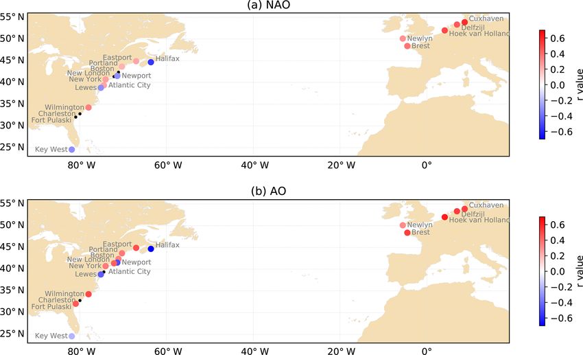
L. Pineau-Guillou et al.: Large-scale changes of the semidiurnal tide                                                                   19

Figure 1. Tide gauges in the North Atlantic. Stations with time series starting before 1940 and longer than 80 years are labelled. Stations
selected for this study are in bold.

   The main characteristics of the 18 selected stations are             fully removed the nodal modulation of M2 amplitude (Si-
summarized in Table 1. Among them, only Brest, Hoek van                 mon, 2007, 2013), as described briefly in Appendix A. Fi-
Holland and Halifax started in the 19th century, in 1846,               nally, 3 station-years were discarded due to problems in the
1879 and 1896 respectively (Table 1, column 2). The number              record (1953 and 1962 at Delfzijl, 1953 at Hoek van Hol-
of years with data for each station varies between 81 and 165           land), and 2 more station-years due to doubtful M2 values
years, Brest being the longest time series (Table 1, column             (1972 at Eastport, 1978 at Newport).
3).                                                                        At all the stations, we computed the normalized M2 am-
                                                                        plitude, removing the average and dividing by the standard
2.1.2   Data processing                                                 deviation over the period 1910–2010:

                                                                                               M2 (t) − M2[1910,2010]
Harmonic analysis was performed in order to compute                     normalized M2 (t) =                           .                (1)
the M2 amplitude. We used the MAS program (Simon,                                                  σM2 [1910,2010]
2007, 2013), developed by the French Hydrographic Office
                                                                        The average M2 and standard deviation σM2 over the 1910–
(SHOM). This program gives results similar to the T_Tide
                                                                        2010 period are given in Table 1 (column 5). The idea is to
harmonic analysis toolbox (Pawlowicz et al., 2002). For in-
                                                                        scale the data in order to compare all the stations together.
stance, Pouvreau et al. (2006) found no differences in the
yearly amplitudes of M2 at Brest over the period 1846 to                2.2     Atmospheric data
2005 using either T_Tide or MAS. Hourly time series were
analysed yearly. Note that at Delfzijl and Hoek van Holland,            2.2.1    Climate indices
data had to be interpolated every hour before 1970, as the
temporal sampling was 3 h. (We checked with hourly time                 We investigated the correlation between secular changes in
series from recent years (1971–2018) that 3-hourly sampling             the tide and climate indices, such as the North Atlantic Os-
did not result in a significant reduction of M2 amplitude in            cillation (NAO) or the Arctic Oscillation (AO) – also called
a tidal analysis compared to hourly sampling.) We processed             Northern Annular Mode (NAM) (Hurrell, 1995; Hurrell and
only years with at least 75 % of data, to avoid seasonal mod-           Deser, 2009; Thompson and Wallace, 2000; Thompson et al.,
ulation affecting the computed amplitudes. In the North At-             2000). These climate indices are related to the distribution of
lantic, M2 is affected by a seasonal variation of a few percent         atmospheric masses. They are based on the difference of av-
(Pugh and Vassie, 1976; Huess and Andersen, 2001; Müller                erage sea-level pressure between two centres of actions (i.e.
et al., 2014; Gräwe et al., 2014). Considering only years with          stations) over long periods (e.g. monthly, seasonal, annual).
at least 75 % of data resulted in excluding up to 15 years                 The NAO is the major pattern of weather and cli-
for a given station (Table 1, columns 3 and 4). We care-                mate variability over the Northern Hemisphere (Hurrell,

https://doi.org/10.5194/os-17-17-2021                                                                      Ocean Sci., 17, 17–34, 2021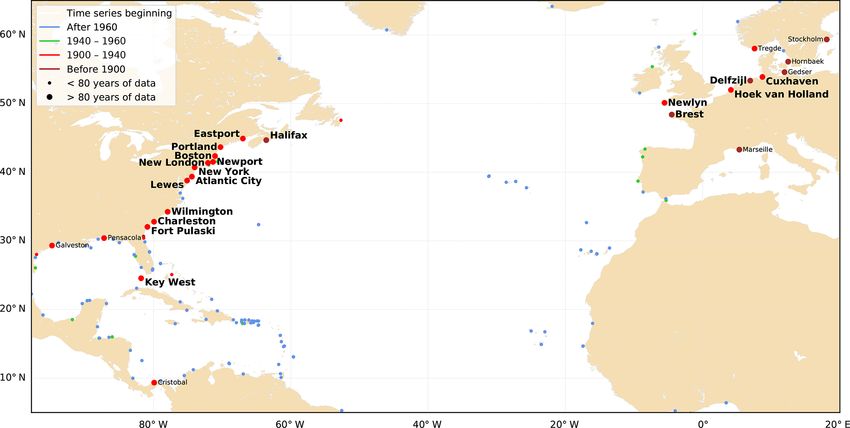
20                                                          L. Pineau-Guillou et al.: Large-scale changes of the semidiurnal tide

Table 1. Main characteristics of tide gauge records selected for this study. Name of the station, time span, number of years with data, number
of years analysed (i.e. with at least 75 % of data), M2 average amplitude and standard deviation over the period 1910–2010, M2 nodal
modulation, estimated trends in M2 amplitude since 1910 and since 1990 up to 2018 in each case (standard errors are 1σ , considering the
noise content in the time series; see text).

                                          Number       Number
     Name                  Time span      of years     of years        M2 (cm)     M2 nod. mod.      M2 trends since     M2 trends since
                                         with data    analysed     [1910–2010]             fnod       1910 (mm/yr)        1990 (mm/yr)
     Cuxhaven             1918–2018           102          101    135.05 ± 3.68             1.8 %        0.68 ± 0.56       −0.47 ± 0.78
     Delfzijl             1879–2018           138          138    125.58 ± 6.96             1.7 %        2.02 ± 0.59       −0.09 ± 0.28
     Hoek van Holland     1900–2018            88           82     76.95 ± 2.63             0.8 %        0.85 ± 0.32       −0.45 ± 0.17
     Newlyn               1916–2016           102           98    170.66 ± 0.75             3.3 %        0.14 ± 0.09       −0.28 ± 0.49
     Brest                1846–2018           165          158    204.54 ± 0.91             3.8 %        0.13 ± 0.11       −0.36 ± 0.18
     Halifax              1896–2012            99           95     62.83 ± 0.64             3.7 %       −0.15 ± 0.05        0.32 ± 0.35
     Eastport             1930–2018            90           82    263.51 ± 2.50             2.5 %        0.80 ± 0.21        1.01 ± 0.65
     Portland             1910–2018           109          104    135.07 ± 1.84             2.8 %        0.56 ± 0.06        0.72 ± 0.23
     Boston               1922–2018            98           96    136.57 ± 1.03             2.9 %        0.27 ± 0.06        0.42 ± 0.24
     Newport              1931–2018            89           84     50.86 ± 0.41             4.1 %       −0.09 ± 0.03       −0.03 ± 0.12
     New London           1939–2018            81           76     35.93 ± 0.25             3.5 %        0.06 ± 0.02        0.03 ± 0.09
     New York             1921–2018            95           80     65.13 ± 0.83             3.7 %        0.33 ± 0.07        0.93 ± 0.15
     Atlantic City        1912–2018           107          101     58.48 ± 0.31             3.8 %        0.00 ± 0.03       −0.18 ± 0.09
     Lewes                1919–2018            85           72     59.91 ± 0.43             3.1 %       −0.06 ± 0.09       −0.33 ± 0.07
     Wilmington           1936–2018            84           82     56.84 ± 6.16             1.7 %        2.51 ± 0.46        1.80 ± 0.44
     Charleston           1901–2018           101          100     76.40 ± 1.33             3.0 %        0.32 ± 0.18       −0.02 ± 0.10
     Fort Pulaski         1936–2018            84           78    100.60 ± 1.01             3.1 %        0.18 ± 0.14       −0.01 ± 0.21
     Key West             1913–2018           106          104     17.50 ± 0.36             2.9 %        0.08 ± 0.04        0.13 ± 0.02

1995; Hurrell and Deser, 2009). Variations of NAO drive                  2.2.2    Sea level pressure
the climate variability over Europe and North America
(Hurrell et al., 2003). We used the wintertime (Decem-                   We employed the Twentieth Century Reanalysis (20CR ver-
ber to March) Hurrell station-based NAO Index (retrieved                 sion 3 dataset) (Compo et al., 2011; Slivinski et al., 2019),
from https://climatedataguide.ucar.edu/climate-data/hurrell-             a historic weather reconstruction from 1836 to 2015, with a
north-atlantic-oscillation-nao-index-station-based, last ac-             1◦ gridded global coverage. However, we made use only of
cess: April 2020). It is based on the difference of normalized           data from 1850 to be more consistent with the temporal cov-
average winter sea-level pressure between Lisbon (Portugal)              erage of the tide gauge measurements. This will be discussed
and Stykkishólmur/Reykjavik (Iceland). The normalization                 in Sect. 4.
involves removing the mean (1864–1983) and dividing by
the long-term standard deviation. The NAO index covers the
                                                                         3     Results
period 1864–2019.
   The Arctic Oscillation (AO) is another index which                    3.1     M2 variations
resembles the NAO index. It is defined as the first EOF
of Northern Hemisphere winter sea-level pressure data                    For the North-East Atlantic, the variations of normalized M2
(Thompson and Wallace, 1998, 2000; Thompson et al.,                      amplitude are presented in Fig. 2a.
2000). The AO index is highly correlated with the NAO.                      The first result is that since 1910, the variations show sim-
We used the wintertime Hurrell AO index (retrieved from                  ilar patterns at all the stations; M2 amplitude decreases up
https://climatedataguide.ucar.edu/climate-data/hurrell-                  to the 1960s, then increases, and decreases again since the
wintertime-slp-based-northern-annular-mode-nam-index,                    1990s. This suggests that these changes are probably due to
last access: April 2020). The AO index covers the period                 large-scale processes, rather than local effects due to changes
1899–2019.                                                               in the environment (e.g. harbour development, dredging, sil-
   To remove the interannual variability and estimate low-               tation) or instrumentation errors. The similar patterns be-
frequency variations, climate indices were low-pass filtered             tween Brest and Cuxhaven may be surprising, as Cuxhaven is
with a 9-year mean filter.                                               located in the North Sea, and not in the open Atlantic Ocean,
                                                                         and far away from Brest, around 1300 km. This indicates
                                                                         that the spatial scale of the processes responsible for these
                                                                         changes must be at least as large as the North-East Atlantic.

Ocean Sci., 17, 17–34, 2021                                                                      https://doi.org/10.5194/os-17-17-2021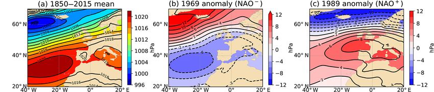
L. Pineau-Guillou et al.: Large-scale changes of the semidiurnal tide                                                                      21

                                                                                                                    .

Figure 2. Normalized annual M2 amplitude (a) in the North-East Atlantic (b) in the North-West Atlantic, stations with positive trends (c) in
the North-West Atlantic, stations with negative or no trend. The stars in (b) in the 1860s correspond to M2 amplitude at Eastport and Portland
from Ray and Talke (2019), and New York from Talke et al. (2014), after normalization (Eq. 1).

Different authors have noticed the increase of tidal range               be sensitive to local effects, such as the migration of the un-
from 1960 to 1990 in the southern North Sea. Hollebrandse                derwater channels and the evolution of the tidal flats (Jacob
(2005) found a gradual increase during the period 1955–1980              et al., 2016). Moreover, Cuxhaven is located in the Elbe es-
at all the stations of the Dutch coast (five stations includ-            tuary, and some river engineering works, such as narrowing
ing Hoek van Holland) and the German coast (seven sta-                   and deepening, may induce tidal amplification (Winterwerp
tions). Mudersbach et al. (2013) found a significant increase            and Wang, 2013; Winterwerp et al., 2013).
in M2 amplitude at Cuxhaven since around the mid-1950s.
Note that Cuxhaven is located in the German Bight; shal-
low depths and the shape of the coastline may induce some
amplification. Variations in M2 at Cuxhaven could therefore

https://doi.org/10.5194/os-17-17-2021                                                                        Ocean Sci., 17, 17–34, 2021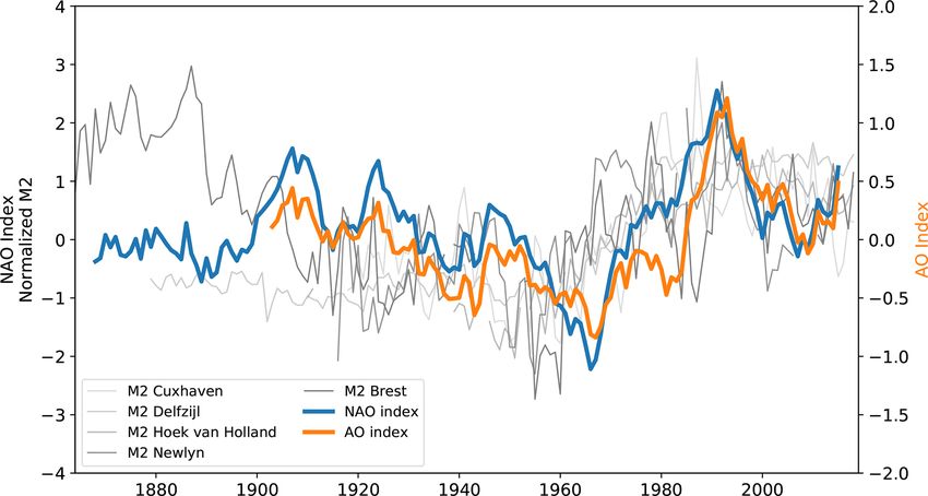
22                                                      L. Pineau-Guillou et al.: Large-scale changes of the semidiurnal tide

   Before 1910, normalized M2 values are higher at Brest           is that M2 amplitude varies differently in the North-West and
than at Delfzijl. The construction of dykes that have grad-        in the North-East Atlantic. The second is that there are dis-
ually closed the harbour of Brest since the end of the 19th        crepancies between stations, even when close to each other
century may have altered the tide at Brest. The high val-          (e.g. Atlantic City and Lewes). We split the stations into two
ues before 1910 may be due to local changes, in addition to        groups, in order to facilitate the detection of patterns, each
large-scale changes. To go further, the potential role of these    being consistent in terms of trends: one with positive trend
successive constructions needs to be investigated (Wikipedia       (group 1 in Fig. 2b), the other one with negative or no trend
contributors, 2020). Cartwright (1972) made a first attempt        (group 2 in Fig. 2c).
to evaluate the influence of reducing the width of access to          The first group (with positive trends) consists of nine sta-
the harbour but did not take into account a potential role of      tions (Fig. 2b). Three outcomes can be highlighted. The first
dredging, for which we have no information. This example           is that M2 amplitude has increased overall since 1900. How-
underlines the complexity of interpretation of the variations      ever, between 1980 and 1990, all the stations slightly de-
when changes of local and large-scale origin occur at the          crease, and since 1990 they have increased again. The second
same time. Note that in the following, we focus mainly on          outcome is that the rate of increase is very different from one
the 20th century, as most of the stations start after 1900 (15     station to another (keeping in mind that M2 is normalized
out of 18 stations).                                               by standard deviation in Fig. 2). Portland is increasing 1.4
   The second result is that there is no obvious linear trend in   times faster than Charleston (standard deviations being re-
M2 variations, but rather break or change points, M2 increas-      spectively of 1.82 and 1.33 cm) and 28 times faster than Key
ing and then decreasing, depending on the periods consid-          West (standard deviation being only 0.36 cm at Key West).
ered. Overall, M2 decreases from 1910 until 1960, increases        The large increase in Portland may be explained by some
again until 1980–1990, to finally decrease since 1990; note        amplification in the Gulf of Maine. In many semienclosed
that the curve flattens between 1920 and 1940. Pouvreau            basins, resonance leads to tidal amplification (Talke and Jay,
et al. (2006) already noticed these variations at Brest and        2020; Haigh et al., 2019). In the Gulf of Maine, Ray and
Newlyn and suggested a long-period oscillation of around           Talke (2019) reported that the tides in the Gulf are in res-
140 years, rather than a steady secular trend. A careful analy-    onance, with a natural resonance frequency close to the N2
sis of the harmonic development of the tidal potential showed      tide (Garrett, 1972; Godin, 1993). Tides may be then very
that no tidal component could explain this oscillation. Sim-       sensitive to any changes in the environment (e.g. basin con-
ilarly, no linear combination of tidal harmonic components         figuration – shape, depth – but also external forcing). The
could explain it (Pouvreau et al., 2006). This indicates that      third outcome, and probably the most interesting one, is re-
these variations are not due to an astronomical component.         lated to the values of M2 at Eastport, Portland and New York
However, in contrast to Brest, M2 at Delfzijl stays flat be-       in the 1860s, estimated from Ray and Talke (2019) and Talke
tween 1880 and 1920. The decrease observed at Brest be-            et al. (2014), and represented (after normalization) as stars
tween 1880 and 1920 may be due to harbour development              in Fig. 2b. These values are not consistent with the positive
and/or dredging (see above). This underlines the importance        linear trends observed since 1900, which provides some con-
of sea level data archaeology, for research studies related to     sistency with the hypothesis formulated from the analyses of
long-term changes (Pouvreau, 2008; Woodworth et al., 2010;         the data prior to the 20th century in Fig. 2a: long-term varia-
Marcos et al., 2011; Talke and Jay, 2013, 2017; Ray and            tions introduce some breaks or change points, M2 increasing
Talke, 2019; Bradshaw et al., 2015, 2020).                         and then decreasing, depending on the periods considered.
   The third result is that changes in M2 have not the same or-    The decrease observed between the 1870s and 1920s at the
der of magnitude at each station (see Fig. B1 in Appendix B        four stations (Brest, Eastport, Portland, New York) suggests
for time series of M2 ). Note that Fig. 2 represents normal-       a possible large-scale signal, in addition to local processes.
ized M2 , i.e. removing the average and dividing by the stan-         The second group (with negative or no trend) consists of
dard deviation. The order of magnitude of unnormalized M2          four stations (Fig. 2c). Two points can be highlighted. The
changes is roughly the same at Brest and Newlyn (standard          first is that M2 decreases overall for Halifax, Newport and
deviations of 0.9 and 0.8 cm respectively, Table 1, column 5),     Lewes. This is less clear for Atlantic City, which is quite
but more than three times larger at Cuxhaven (standard devi-       noisy and shows no significant trend. The second point is that
ation of 3.7 cm), and even larger at Delfzijl (standard devia-     at Halifax, M2 values in 1896–1897 are higher than those af-
tion of 7 cm). This suggests that the North Sea may be more        ter 1920. This suggests that the decrease may have started
sensitive to the processes responsible for these changes. Note     before the 20th century. However note that at Halifax, there
also that the environmental setting of Cuxhaven and Delfzijl       is a long gap in the data recording (1898–1919), which raises
in the Elbe and Ems estuaries, respectively, could introduce       the possibility of an instrumentation origin in the observed
some amplification (Winterwerp and Wang, 2013; Winterw-            decrease of the M2 amplitude.
erp et al., 2013).
   For the North-West Atlantic, the variations of normalized
M2 amplitude are presented in Fig. 2b and c. The first feature

Ocean Sci., 17, 17–34, 2021                                                             https://doi.org/10.5194/os-17-17-2021
L. Pineau-Guillou et al.: Large-scale changes of the semidiurnal tide                                                          23

3.2   Estimated trends                                              post-1910 negative trends (Table 1, columns 7 and 8). In the
                                                                    North-East Atlantic, they all switch from positive to negative
We estimated the trends for M2 amplitude at each station, us-       trends. This underlines (1) some spatially coherent changes
ing linear regression. We computed the trends over two pe-          in recent decades (Müller, 2011; Ray and Talke, 2019) and
riods: 1910–2018, which corresponds roughly to the whole            (2) the difficulty in estimating long-term trends from short
period of data (only five stations start before 1910), and          records (i.e. less than 30 years), especially if the data are
1990–2018, which corresponds to recent decades. Some tests          noisy (interannual variability) and the underlying processes
showed that the later results were not very sensitive to the        non-linear (change points).
start date (moving 1990 to 1985 or 1995). The trend uncer-             The trends have to be interpreted very carefully as the M2
tainties were estimated considering the noise content in the        variations are not linear and may increase or decrease de-
time series using SARI software (Santamaría-Gómez, 2019).           pending on the years; as a consequence, the estimated trends
The noise was modelled as a white plus power-law noise,             depend strongly on the period considered to estimate it. The
whose spectral index was found to be close to −1 (flicker           interannual variability also plays an important role, and when
noise). The results are summarized in Table 1 (columns 7            substantial, trends can vary depending on the computational
and 8) and Figs. 3 and 4.                                           period. For example, at Cuxhaven, the large interannual vari-
   The trends estimated since 1910 vary significantly from          ability leads to a large uncertainty on the trend computed
one station to another (Fig. 3). They are positive overall (up      since 1990 (−0.47 ± 0.78 mm/yr).
to 2.5 mm/yr at Wilmington), which is consistent with pre-
vious findings (Araújo and Pugh, 2008; Ray, 2009; Wood-
worth, 2010; Müller et al., 2011; Ray and Talke, 2019).             4     Discussion
They are slightly negative at three stations (Halifax, New-
                                                                    4.1    Possible link with mean sea level rise
port, Lewes), and one station shows no trend (Atlantic City).
The estimates are statistically consistent with those found         The MSL rise could partly explain M2 changes. Simulations
previously by different authors (e.g. 0.14 ± 0.09 mm/yr at          show that MSL rise can result in an change of M2 up to
Newlyn compared to 0.19 ± 0.03 mm/yr in Araújo and                  ±10 % of the rise (Pickering et al., 2017; Idier et al., 2017;
Pugh (2008), 0.56 ± 0.06 mm/yr in Portland, compared to             Schindelegger et al., 2018). Schindelegger et al. (2018) show
0.59 ± 0.04 mm/yr in Ray and Talke, 2019). Note that our er-        that the sign of the observed M2 trend is correctly reproduced
ror bars are larger, because we considered the noise content        at 80 % of the tide gauges on a global scale, but their simu-
in the time series as a white noise plus power law noise (we        lated trends tend to differ from observations by a factor of
obtained the same error bars considering white noise only).         3 to 5; i.e. their simulations underestimate the M2 response
In the North-East Atlantic, the trends are consistent with each     to MSL rise in terms of magnitude. Schindelegger et al.
other (in terms of sign), which is not surprising as the stations   (2018) conclude that “magnitudes of observed and modeled
vary similarly (Fig. 2a).                                           M2 trends are within a factor of 4 (or less) from each other
   The largest trends since 1910 are mainly observed in semi-       in nearly 50 % of the considered cases”. The large discrep-
closed basins: Wilmington in the Cape Fear River estuary,           ancies between the simulations and the observations strongly
Delfzijl in Ems estuary, Cuxhaven in Elbe estuary, and East-        suggest that MSL rise is not the only process that may ex-
port and Portland in the Gulf of Maine. This suggests a             plain M2 changes – other large-scale processes, in addition
possible amplification due to resonance effects (e.g. Gulf          to local processes, may also play a role.
of Maine) and/or propagation in shallow waters (e.g. Cux-              Figure 5 shows the annual MSL, after removing the aver-
haven), in addition to local effects. The stations located in es-   age over the period 1910–2010 and filtering with 9-year time
tuaries or in a harbour with a channel may have been subject        windows. The correlations between M2 and MSL indicate
to dredging. Channel deepening increases the water depths,          that M2 varies strongly with MSL (see Sect. 4.2). However,
which reduces the effective drag and leads to tidal range am-       M2 variations show some variability in the North-East At-
plification. This effect may be particularly large in estuar-       lantic (Fig. 2a), which may not be explained with MSL rise
ies (Ralston et al., 2019; Talke and Jay, 2020) and may ex-         alone.
plain the larger trends at Wilmington (Familkhalili and Talke,
2016) and Delfzijl. Finally, the shifting locations of am-          4.2    Possible link with MSL and climates indices
phidromic points could also play a role (Haigh et al., 2019).
In the North Sea, different authors show a possible migration       Processes other than MSL rise may impact the tide (see
of the present-day amphidromes, under a 2 m sea-level rise          Sect. 1), such as the atmospheric circulation and the ocean
scenario (Pickering et al., 2012; Idier et al., 2017).              stratification. Ocean and atmosphere are fully coupled, and
   The trends estimated since 1990 are quite different from         air–sea fluxes are responsible for the exchange of momen-
those estimated since 1910 (Figs. 3 and 4), with more sta-          tum, water (evaporation and precipitation budget) and heat
tions with negative trends: 9 stations out of 18 have post-         at their interface. Among the wide range of possible interac-
1990 negative trends, whereas only 3 stations out of 18 have        tions, two mechanisms have been explored for their ability

https://doi.org/10.5194/os-17-17-2021                                                               Ocean Sci., 17, 17–34, 2021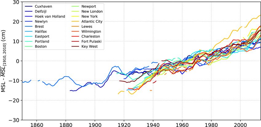
24                                                       L. Pineau-Guillou et al.: Large-scale changes of the semidiurnal tide

Figure 3. Estimated trends in M2 amplitude over the period 1910–2018.

Figure 4. Estimated trends in M2 amplitude over the period 1990–2018.

to modify the tide: (1) the momentum flux (wind stress) and             The NAO index varies from positive to negative phases. Fil-
the gradient of sea level pressure which act on the barotropic          tering the interannual variability, the NAO index tends over-
tide and (2) the water and heat fluxes which induce changes             all to decrease between 1910 and 1970, then increase until
in both temperature and salinity distribution in the ocean. The         1990, and once again decrease. In the same way, M2 ampli-
latter effect acts on the stratification, which in turn could im-       tude tends to decrease up to 1960, then increase until 1990,
pact the tide in two different ways. The first way is the in-           and once again decrease. These similar patterns raise a possi-
ternal tide generation which transfers energy from barotropic           ble connection between NAO and M2 variation, already men-
and baroclinic motion and modifies surface tidal expression             tioned by Müller (2011) on the basis of qualitative criteria. In
(Colosi and Munk, 2006). However, in the present study,                 the following, we provide quantitative insights into the pos-
most of the observations come from coastal stations sheltered           sible influence of NAO.
by wide continental shelves which dampen internal waves.                   We computed the correlations (r value) between normal-
More important is the second way: the stratification acts on            ized M2 and climate indices, NAO and AO (Fig. 7). M2 , NAO
the eddy viscosity profile by modifying current profiles and            and AO are filtered using the same time window (9 years).
bottom drag over continental shelves, which in turn modifies            The correlations are computed since 1910, to have similar
the M2 surface expression (Kang et al., 2002; Müller, 2012;             periods for all the stations. The correlations are considered as
Katavouta et al., 2016).                                                significant only if the p value is lower than 0.05 (95 % sig-
   Here, we focus on the effect of the atmospheric circulation          nificance level). (Note that other statistics to measure the de-
on the tide. We used pressure indices (NAO and AO) that are             gree of association between the M2 and NAO (AO) quantities
relevant to represent atmospheric circulation. The NAO in-              would be worth exploring, for instance, nonlinear association
dex represents the difference of normalized sea level pressure          using Spearman’s correlation coefficient. In this respect, our
between the Azores high pressure system and the Iceland low             study should be regarded as a first step that identifies sites
pressure one (Hurrell, 1995). It indicates the redistribution of        worth considering in future investigations, especially inves-
atmospheric masses between the subtropical Atlantic and the             tigating causal relationships with physics-based modelling.)
Arctic (Hurrell and Deser, 2009). In the North-East Atlantic,           The results are the following: (1) for NAO, 14 stations out of
the similarity between the variations of the low-frequency              18 show significant correlation. Note that at Brest, the corre-
winter NAO index and those of M2 (Fig. 6) suggests a possi-             lation is significant since 1910, but not since 1864 (the NAO
ble impact of large-scale atmospheric circulation on the tide.          index used in this study starts only in 1864). This can be ex-

Ocean Sci., 17, 17–34, 2021                                                                   https://doi.org/10.5194/os-17-17-2021
L. Pineau-Guillou et al.: Large-scale changes of the semidiurnal tide                                                              25

Figure 5. Annual mean sea levels (MSLs), after removing the average over the period 1910–2010. MSL values are filtered using 9-year
windows.

Figure 6. Low-frequency winter NAO and AO indices, obtained with a 9-year mean filter. Normalized annual M2 amplitudes in the North-
East Atlantic (from Fig. 2a) are also plotted in grey.

plained by the M2 larger amplitude over all the 19th century,       sion model (model 2). Models 1 and 2 may be expressed as
which decreases between 1890 and 1910 (Fig. 2a), possi-
                                                                    Model 1 = α1 MSL                                              (2)
bly due to harbour development and construction of dykes
(see Sect. 3.1). (2) In the North-East Atlantic, all the sta-       Model 2 = αMSL + βNAO.                                        (3)
tions are positively correlated with NAO. (3) The strongest            The correlations between M2 and model 1 (MSL) and
correlations (i.e. greater than 0.5) are in the northern part of    model 2 (NAO and MSL) are presented in Fig. 8. We checked
the North Atlantic, with strong positive correlations at Cux-       if there was correlation between NAO and MSL at the sta-
haven and Hoek van Holland and strong negative correlation          tions: there is no correlation at six stations, and r value is be-
at Halifax (−0.55). (4) For AO, we found similar, but overall       tween 0.2 and 0.6 at eight stations; see Fig. 8 and discussion
larger, r values. This is not surprising as these two indices       below. The results are the following: (1) M2 varies at first
are closely related.                                                order with MSL (Fig. 8). (2) The introduction of the NAO
   To go further in the relative contribution of MSL and NAO        (model 2) allows increasing the predictive performance of
in M2 variability, we fitted two linear regression models on        the model, beyond the inherent effect of adding an additional
M2 variations. In the following, M2 , MSL and NAO are fil-          regression parameter. Indeed, on average, the Akaike infor-
tered over 9-year time windows and normalized. At all the           mation criterion (AIC) is 99.9 for model 2, instead of 112.7
stations, we fitted M2 variations with a MSL linear regression      for model 1. On average, the r 2 value is 0.67 for model 2
model (model 1) and a MSL and NAO multiple linear regres-           instead of 0.61 for model 1. At some stations, the increase

https://doi.org/10.5194/os-17-17-2021                                                                 Ocean Sci., 17, 17–34, 2021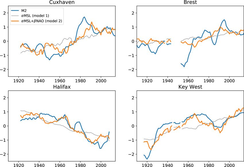
26 L. Pineau-Guillou et al.: Large-scale changes of the semidiurnal tide
Figure 7. Correlation (r value) since 1910 between M2 and (a) North Atlantic Oscillation and (b) Arctic Oscillation. Black dots are stations
with no significant correlation. M2 , NAO and AO are filtered using the same time window (9 years).
(orange bars in Fig. 8). For example, at Hoek van Holland,
the relative NAO contribution is very small, mainly because
MSL and NAO are highly correlated (r = 0.59). Figure 10
shows M2 variations along with the predictions from the two
models, at all four stations where the NAO contribution is
β
significant ( α+β > 0.25), and the correlation between M2
and model 2 is large enough (r > 0.3). At Cuxhaven, Halifax
and Key West, model 2 (MSL- and NAO-dependent) natu-
rally captures the M2 variations better than model 1 (MSL-
dependent); at Brest, the improvement is less significant. The
trend switch observed since 1990 in the North-East Atlantic
could be partly explained by the influence of the NAO on the
tide.
These results suggest that a NAO-related mechanism may
explain part of the variability of M2 . As mentioned by Müller
Figure 8. Variance explained (r 2 value) since 1910 between M2 and
(2011), “it is shown that sea-level, sea surface temperature
NAO, M2 and MSL, M2 and fitted model αMSL + βNAO (model and Arctic ice thickness are correlated with the NAO index.
2), NAO and MSL. M2 , NAO and MSL are filtered using the same Thus, changes in the dynamics of the atmosphere could af-
time window (9 years). Note that there is no orange bar for NAO– fect both M2 and S2 tides by processes discussed under (1),
MSL when the correlation is not significant (p > 0.05). (2) and (3).” An underlying mechanism linked with (2) – sea
surface temperature – could be changes in the ocean strati-
fication. This is one of main possible hypotheses invoked in
is quite large. For example at Cuxhaven, the r 2 value jumps Ray and Talke (2019) to explain secular changes in M2 am-
β
from 0.42 to 0.64 between model 1 and 2. (3) The ratio α+β plitude in the Gulf of Maine; this is also the main hypothesis
represents roughly the relative contribution of the NAO com- in Müller et al. (2014) and Gräwe et al. (2014) to explain
pared to the total effect of MSL and NAO (Fig. 9), as MSL seasonal modulation of M2 in the North Sea. The relation-
and NAO are normalized. We found a significant contribu- ship between the NAO index and stratification is complex
tion at some stations (e.g. more than 30 % at Cuxhaven and and spatially variable across the North-East Atlantic (Fro-
Halifax), whereas it is negligible at others (e.g. only 5 % at mentin and Planque, 1996). In the North Sea, the sea surface
Portland). A total of 8 stations out of 18 show large NAO temperatures are positively correlated with NAO (Becker and
contribution (> 20 %). The North-East Atlantic seems to be Pauly, 1996), while subsurface temperatures show no signif-
more sensitive to the NAO. Note that the interpretation of the icant correlation with NAO (Tian et al., 2016). Stratification
results is tricky when MSL–NAO correlation is significant
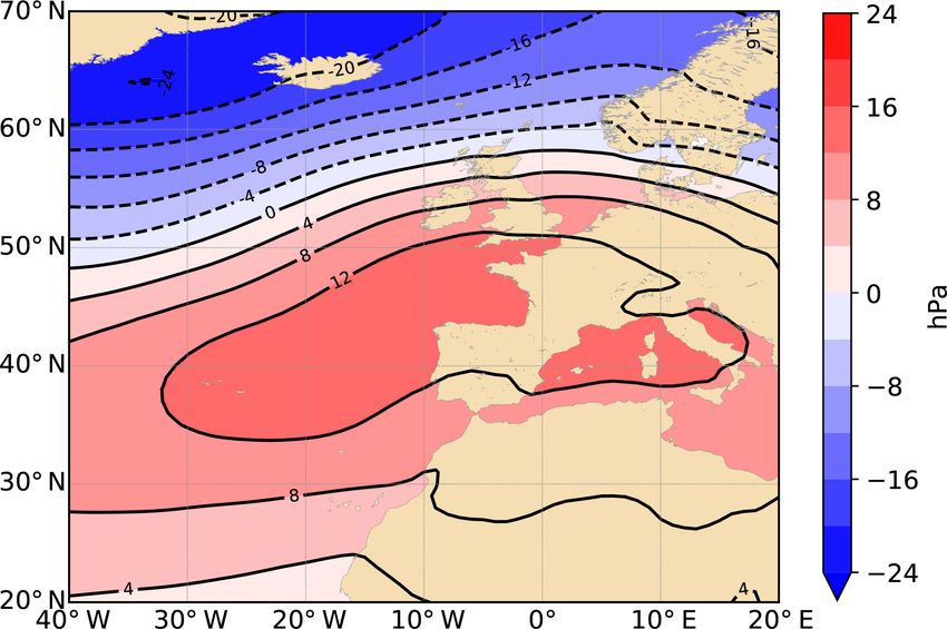
Ocean Sci., 17, 17–34, 2021 https://doi.org/10.5194/os-17-17-2021L. Pineau-Guillou et al.: Large-scale changes of the semidiurnal tide 27 Figure 9. Relative contribution of α compared to β in the fitted model αMSL + βNAO. Black dots are stations with no significant M2 –NAO correlation. The size of each large dot is proportional to the correlation between M2 and the fitted model. Stations with no MSL–NAO correlations are labelled in bold. Figure 10. Variations since 1910 of M2 , αMSL (model 1), αMSL+ βNAO (model 2). M2 , NAO and MSL are filtered using the same time window (9 years). could therefore be (positively) correlated with NAO, but a tides and meteorological fields rather than with tides only. dedicated study, outside the scope of this paper, would be Figure 11a shows the average sea-level pressure during the necessary. Another underlying mechanism linked this time period 1850–2015, derived from the Twentieth Century Re- with (1) – sea level – could be the difference of spatial dis- analysis (20CR) (Compo et al., 2011; Slivinski et al., 2019). tribution of water level, due to different sea-level pressure A positive NAO winter (e.g. 1989) corresponds to a situa- and wind stress patterns. This is the hypothesis invoked in tion with a stronger pressure gradient than average, between Huess and Andersen (2011) to explain the seasonal modula- the two pressure systems of Azores and Iceland (Fig. 11c). tion of M2 in the North Sea. They ran a barotropic model, By contrast, a negative NAO winter (e.g. 1969) corresponds forced with tides only and with both tides and meteorolog- to a weaker gradient pressure than usual (Fig. 11b). (We de- ical fields; their results show that the M2 seasonal modula- fine winter here as December–February.) This way, from one tion is better captured when the model is forced with both year to another, the large-scale atmospheric masses are dis- https://doi.org/10.5194/os-17-17-2021 Ocean Sci., 17, 17–34, 2021
28                                                       L. Pineau-Guillou et al.: Large-scale changes of the semidiurnal tide

tributed differently, and as a consequence, the water volumes       lantic suggests a possible influence of the large-scale atmo-
are also distributed differently in the North Atlantic. In a sit-   spheric circulation on the tide. Our statistical analysis con-
uation of NAO+ , the surface waters are pushed onshore by           firms large correlations at all the stations in the North-East
westerly winds, moving from Iceland to the European coasts          Atlantic. The trend switch observed since 1990 could be
of France, Spain and Portugal. Figure 12 shows the redistri-        the signature of the large-scale atmospheric circulation on
bution of the sea-level pressure, between two years with high       the M2 tide. The underlying mechanism would be a differ-
and low NAO indices (here 1989 and 1969). Note that this is         ent spatial distribution of water level from one year to an-
an extreme situation, as these years have strong positive and       other, depending on the low-frequency sea-level pressure pat-
negative indices. Assuming an inverse barometer response            terns, and impacting the propagation of the tide in the North
of sea level, the changes in terms of water level may vary          Atlantic basin. In the future, dedicated modelling studies
from more than 24 cm in the northwestern part of the area to        should be undertaken to confirm or discard this hypothesis.
around −12 cm in the region that includes most of the North-        These simulations should also allow estimating the effect of
East Atlantic tide gauges considered in this study. This vari-      the wind (through the Ekman current) and currents on M2
ation of a few tens of centimetres is probably negligible off-      changes (Devlin et al., 2018).
shore but may have some impact on tide propagation along               In this study, we focused only on M2 amplitude. A similar
the continental shelves and in shallow waters. It could also        analysis on the phase lag would draw a more complete pic-
shift slightly the amphidromic points. Assuming that these          ture of the M2 variations (Müller, 2011; Woodworth, 2010;
changes have a similar impact (in terms of magnitude) on            Ray and Talke, 2019). Other constituents are also affected.
M2 as MSL changes, that is, ±10 % in shallow waters ac-             Results show that S2 amplitude decreases at all the stations
cording to recent simulations (Pickering et al., 2017; Idier        located in the North-West Atlantic and, in contrast, tends to
et al., 2017), we find that they can yield centimetric changes      increase in the North-East Atlantic (not shown). The large-
in M2 amplitude. In other words, their order of magnitude is        scale decrease of S2 observed in the North-West Atlantic is
roughly in agreement with the changes observed in M2 (Ta-           consistent with previous studies (e.g. Ray, 2006, in the Gulf
ble 1). However, it is difficult to disentangle the effects of      of Maine). Further investigations should be definitely con-
stratification and meteorological forcing (sea-level pressure       ducted to extend this work to more constituents.
and wind stress) in M2 changes, and possibly both mecha-               The historic data show that the changes started long before
nisms coexist. Dedicated simulations should be conducted to         the 20th century. This conclusion would not have been pos-
assess the effects of atmospheric forcing on M2 variability.        sible without the huge work of data rescue undertaken over
                                                                    the past decades (e.g. Pouvreau et al., 2006; Pouvreau, 2008;
                                                                    Bradshaw et al., 2016). This underlines the great importance
5    Conclusions                                                    of sea level data archaeology, which allows extending and
                                                                    improving historical datasets (Pouvreau, 2008; Woodworth
We investigated the long-term changes of the principal tidal        et al., 2010; Marcos et al., 2011; Talke and Jay, 2013, 2017;
component M2 over the North Atlantic coasts. We analysed            Ray and Talke, 2019; Bradshaw et al., 2015, 2020; Haigh
18 tide gauges with time series starting no later than 1940.        et al., 2019). This is essential for studies related to climate
The longest is Brest with 165 years of data. We carefully pro-      change.
cessed the data, particularly to remove the 18.6-year nodal            Finally, we should mention several additional limitations
modulation.                                                         and perspectives in this study. (1) We processed the time se-
   We found that M2 variations were consistent at all the sta-      ries considering that they were quality controlled. A fuller
tions in the North-East Atlantic (Cuxhaven, Delfzijl, Hoek          analysis of the data quality before processing would prob-
van Holland, Newlyn, Brest), whereas variations appear be-          ably be valuable. (2) We did not investigate the history of
tween stations in the North-West Atlantic. The changes              each station. There are probably some local changes (e.g.
started long before the 20th century and are not linear. The        environment or instrumentation) that may explain a part of
trends vary significantly from one station to another; they         the variability of M2 amplitude and some discrepancies be-
are overall positive, up to 2.5 mm/yr, or slightly negative.        tween stations. (3) The tide gauges are located mainly in
Since 1990, in many stations, the trends switch from posi-          harbours. They are affected at the same time by local- and
tive to negative values. The significant differences between        regional/global-scale changes, which are difficult to sepa-
the trends since 1910 and 1990 indicate caution when inter-         rate. Moreover, they may not be representative of changes
preting trends based on short records, i.e. less than 30 years,     offshore. A similar study based on satellite altimetry data
especially if the data are noisy (interannual variability) and      would probably be of great interest, even if temporal scale
the underlying processes non-linear (change points).                for satellite data is still rather short (i.e. < 30 years) com-
   Concerning the causes of the observed changes, M2 varies         pared to climate-scale processes. (4) We focused mainly on
primarily with the MSL, but MSL rise is not sufficient to ex-       the UHSLC dataset, which consists of 249 stations in the At-
plain the variations alone. The similarity between the North        lantic Ocean. Other relevant stations (which are not in this
Atlantic Oscillation and M2 variations in the North-East At-        dataset) may be considered in future studies. (5) We did not

Ocean Sci., 17, 17–34, 2021                                                              https://doi.org/10.5194/os-17-17-2021
L. Pineau-Guillou et al.: Large-scale changes of the semidiurnal tide 29 Figure 11. Winter sea-level pressure over the North-East Atlantic (a) average over 1850–2015 (b) anomaly in 1969 (NAO− ) (c) anomaly in 1989 (NAO+ ). Contour intervals are every 2 hPa. Figure 12. Difference of winter sea-level pressure between 1989 (NAO+ ) and 1969 (NAO− ) over the North-East Atlantic. Contour intervals are every 4 hPa. investigate the impact of storminess on the tide. Dedicated studies are necessary to estimate if changes in storminess could affect significantly tidal constituents. (6) We used only winter AO and NAO indices, which show more variability than annual indices. A similar analysis with annual indices shows similar results for the correlation with AO or NAO (positive correlation on the North-East Atlantic). With an- nual rather than monthly indices, the difference of pressure fields will decrease, and as a consequence, the magnitude of the sea-level response will also decrease. Further investiga- tions should be conducted on this point. https://doi.org/10.5194/os-17-17-2021 Ocean Sci., 17, 17–34, 2021
30 L. Pineau-Guillou et al.: Large-scale changes of the semidiurnal tide
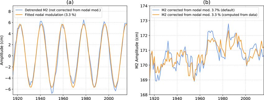
Appendix A: Nodal modulation The negative of the mean longitude of the Moon ascending
node is expressed simply as a function of time (p. 116 in
The M2 component is subject to a 18.6-year modulation, Simon, 2007, p. 112 in Simon, 2013):
separated from a neighbouring line in the tidal potential
(m2 ) whose Doodson number differs in its fifth frequency N 0 = −N = 234.555 + 1934.1363T + 0.0021T 2 , (A4)
(255 555 and 255 545 for M2 and m2 , respectively) (Doodson
and Warburg, 1941; Pugh and Woodworth, 2014). This fifth with N 0 in degrees, and T the time elapsed since 1 January
frequency corresponds to N 0 , the negative of the mean longi- 2000 at 12:00, expressed in Julian centuries (36 525 d).
tude of the Moon ascending node – hence the “nodal” term The tidal program we used (MAS) corrected M2 apply-
– whose period is 18.6 years. Note that there is also another ing the usual 3.7 % nodal modulation (Eq. A3). However,
component close to M2 , whose Doodson number differs only this value may vary significantly from one station to another;
from the fifth frequency (255 565), but it is negligible, its Ray (2006) reported values ranging from 2.3 % to 3.6 % in
amplitude in the tidal potential being only 0.05 % of M2 , the Gulf of Maine. Here, we computed directly fnod from the
whereas m2 amplitude is 3.7 % of M2 (Simon, 2007, 2013). observed data, proceeding as follows. (1) We added the de-
With one year of hourly data, the two components M2 and m2 fault nodal correction 1 + 0.037 cos(N 0 + π ) to the M2 varia-
cannot be separated by a yearly harmonic analysis (at least tions. (2) We detrended the obtained signal removing the last
18.6 years are necessary). As a consequence, M2 amplitude intrinsic mode function (IMF) of an empirical mode decom-
is modulated by m2 . However, we can estimate this modu- position (EMD) (Huang et al., 1998); note that the EMD is
lation and remove it. The harmonic formulation is expressed an analysis tool which partitions a series into “modes” (i.e.
schematically as a sum of harmonic components: IMFs), the last one being the trend of the signal. (3) We fit-
X ted a function am2 cos(N 0 + π ) to this detrended signal to
h(t) = ai cos(Vi (t) − κi ), (A1) estimate am2 , N 0 being expressed as in Eq. (A4). (4) We fi-
i nally computed fnod as the ratio between m2 and M2 ampli-
where h(t) is the sea level height at time t, Vi (t) is the astro- tudes (Eq. A3). Figure A1a shows an example of estimate of
nomical argument (computed from Doodson number) and ai , M2 modulation at Newlyn: the fit leads to a nodal modula-
κi the amplitude and phase lag of each component. Consider- tion of 3.3 %. Note that this value is consistent with Wood-
ing that M2 and m2 are very close in terms of frequency, we worth (2010) (3.2 %), whereas Woodworth et al. (1991) gave
can assume that their phase lags are similar (κM2 ' κm2 ). As a slightly different value (2.8 %). Figure A1b shows the im-
their difference of astronomical arguments is Vm2 − VM2 = pact of this value rather than the default one: oscillations of
N 0 + π , the M2 and m2 contributions to the total water level 18.6 years are clearly reduced. Note that in this study, the
may be expressed as m2 amplitude – and then the nodal correction – could have
been computed from the full time series harmonic analysis,
hM2 (t) + hm2 (t) = hM2 (t)[1 + fnod cos(N 0 + π )], (A2) as records are longer than 18.6 years. However, the method
presented here to compute the nodal correction can be ap-
where fnod , the nodal modulation, is the ratio of the ampli- plied even for time series shorter than 18.6 years.
tude of m2 and M2 . As M2 and m2 are very close in terms of The computed nodal modulations are summarized in Ta-
frequency, fnod is generally considered as close to the ratio ble 1 (column 6). They vary from 0.8 % to 4.1 %. Note that
of their amplitude in the tidal potential, Am2 and AM2 : these values are consistent with those obtained by previous
authors (Ray, 2006; Müller, 2011; Woodworth, 2010; Ray
am2 Am 2
fnod = ' ' 0.037. (A3) and Talke, 2019). Only the value at Charleston differs sig-
aM2 AM2 nificantly: 3.0 % in our study compared to 3.7 % in Müller
(2011).
Figure A1. (a) Estimation of the nodal modulation of M2 amplitude (mean removed) at Newlyn. (b) Impact on M2 amplitude of the nodal
modulation correction at Newlyn. M2 is detrended in (a) to better fit the nodal modulation.
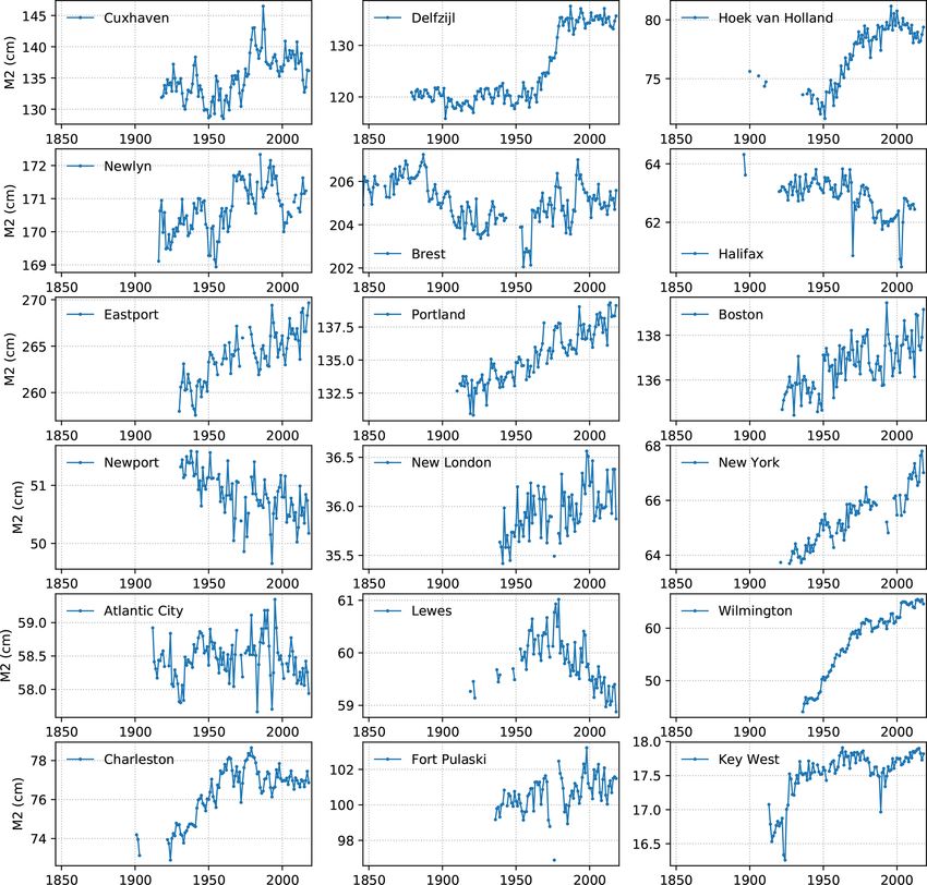
Ocean Sci., 17, 17–34, 2021 https://doi.org/10.5194/os-17-17-2021L. Pineau-Guillou et al.: Large-scale changes of the semidiurnal tide 31 Appendix B: Time series of annual M2 amplitude at all the stations Figure B1. Annual M2 amplitude at the 18 selected tide gauges. https://doi.org/10.5194/os-17-17-2021 Ocean Sci., 17, 17–34, 2021
32                                                          L. Pineau-Guillou et al.: Large-scale changes of the semidiurnal tide

Data availability. The tide gauge data are available at University      Review statement. This paper was edited by Philip Woodworth and
of Hawaii Sea Level Center ftp://ftp.soest.hawaii.edu/uhslc/            reviewed by Stefan Talke and one anonymous referee.
rqds/atlantic (Caldwell et al., 2015). The NAO climate index
is available at https://climatedataguide.ucar.edu/climate-data/
hurrell-north-atlantic-oscillation-nao-index-station-based
(Hurrell and the National Center for Atmospheric Re-                    References
search Staff, 2020). The AO climate index is avail-
able        at       https://climatedataguide.ucar.edu/climate-data/    Araújo, I. B. and Pugh, D. T.: Sea levels at Newlyn 1915–2005:
hurrell-wintertime-slp-based-northern-annular-mode-nam-index              Analysis of trends for future flooding risks, J. Coast. Res., 24,
(National Center for Atmospheric Research Staff, 2020). The               203–212, https://doi.org/10.2112/06-0785.1, 2008.
Twentieth Century Reanalysis Project version 3 dataset is available     Becker, G. A. and Pauly, M.: Sea surface temperature changes in
at     https://www.psl.noaa.gov/data/gridded/data.20thC_ReanV3.           the North Sea and their causes, ICES J. Mar. Sci., 53, 887–898,
monolevel.html#caveat (Slivinski et al., 2019).                           https://doi.org/10.1006/jmsc.1996.0111, 1996.
                                                                        Bradshaw, E., Rickards, L., and Aarup, T.: Sea level data archaeol-
                                                                          ogy and the Global Sea Level Observing System (GLOSS), Geo-
Author contributions. LPG analysed the data and wrote the paper.          resj., 6, 9–16, https://doi.org/10.1016/j.grj.2015.02.005, 2015.
PL contributed to the interpretation of the data and the writing of     Bradshaw, E., Woodworth, P., Hibbert, A., Bradley, L., Pugh, D.,
the paper. GW contributed to the analysis and interpretation of the       Fane, C., and Bingley, R.: A century of sea level measurements
data and the writing of the paper.                                        at Newlyn, Southwest England, Mar. Geodesy, 39, 115–140,
                                                                          https://doi.org/10.1080/01490419.2015.1121175, 2016.
                                                                        Bradshaw, E., Ferret, Y., Pons, F., Testut, L., and Woodworth,
                                                                          P.: Workshop on sea level data archaeology, Technical Report,
Competing interests. The authors declare that they have no conflict
                                                                          Workshop Report No. 287, Intergovernmental Oceanographic
of interest.
                                                                          Commission, Paris, France, 47 pp., 2020.
                                                                        Caldwell, P. C., Merrifield, M. A., and Thompson, P. R.: Sea level
                                                                          measured by tide gauges from global oceans – the Joint Archive
Special issue statement. This article is part of the special              for Sea Level holdings (NCEI Accession 0019568), Version
issue “Developments in the science and history of tides                   5.5, NOAA National Centers for Environmental Information,
(OS/ACP/HGSS/NPG/SE inter-journal SI)”. It is not associ-                 Dataset, ftp://ftp.soest.hawaii.edu/uhslc/rqds/atlantic, 2015.
ated with a conference.                                                 Cartwright, D. E.: Secular changes in the oceanic tides
                                                                          at Brest, 1711–1936, Rev. Geophys., 57, 433–449,
                                                                          https://doi.org/10.1111/j.1365-246X.1972.tb05826.x, 1972.
Acknowledgements. The sea level observations were provided by           Colosi, J. A. and Munk, W.: Tales of the venerable Hon-
the University of Hawaii Sea Level Center – retrieved from ftp://ftp.     olulu tide gauge, J. Phys. Oceanogr., 36, 967–996,
soest.hawaii.edu/uhslc/rqds (last access: April 2020). The sea level      https://doi.org/10.1175/JPO2876.1, 2006.
data at Delfzijl and Hoek van Holland were provided by Rijkswater-      Compo, G. P., Whitaker, J. S., Sardeshmukh, P. D., Matsui, N., Al-
staat (RWS) Service Desk, Netherlands. The climate indices (NAO           lan, R. J., Yin, X., Gleason, B. E., Vose, R. S., Rutledge, G.,
and AO indices) were provided by the Climate Analysis Section,            Bessemoulin, P., Brönnimann, S., Brunet, M., Crouthamel, R. I.,
NCAR, Boulder, USA – retrieved from https://climatedataguide.             Grant, A. N., Groisman, P. Y., Jones, P. D., Kruk, M., Kruger,
ucar.edu/climate-data/ (last access: April 2020). The harmonic anal-      A. C., Marshall, G. J., Maugeri, M., Mok, H. Y., Nordli, Ø., Ross,
ysis program MAS was provided by the French Hydrographic Of-              T. F., Trigo, R. M., Wang, X. L., Woodruff, S. D., and Worley,
fice (SHOM). Support for the Twentieth Century Reanalysis Project         S. J.: The twentieth century reanalysis project, Q. J. Roy. Meteo-
version 3 dataset was provided by the US Department of Energy,            rol. Soc., 137, 1–28, https://doi.org/10.1002/qj.776, 2011.
Office of Science Biological and Environmental Research (BER),          Devlin, A. T., Zaron, E. D., Jay, D. A., Talke, S. A., and Pan, J.: Sea-
by the National Oceanic and Atmospheric Administration Climate            sonality of tides in Southeast Asian waters, J. Phys. Oceanogr.,
Program Office, and by the NOAA Physical Sciences Laboratory.             48, 1169–1190, https://doi.org/10.1175/JPO-D-17-0119.1, 2018.
The authors very warmly thank the two reviewers (Stefan Talke           Doodson, A. T.: Perturbations of harmonic tidal constants, P. R. Soc.
and an anonymous reviewer) and the editor (Philip Woodworth) for          A, 106, 513–526, https://doi.org/10.1098/rspa.1924.0085, 1924.
their careful reading and their many constructive comments, which       Doodson, A. T. and Warburg, H. D.: Admiralty manual of tides,
greatly improved the paper.                                               HMSO, London, UK, 1941.
                                                                        Familkhalili, R. and Talke, S. A.: The effect of chan-
                                                                          nel deepening on tides and storm surge: A case study
Financial support. This research has been supported by the French         of Wilmington, NC, Geophys. Res. Lett., 43, 9138–9147,
Research Institute for Exploitation of the Sea (IFREMER) and by           https://doi.org/10.1002/2016GL069494, 2016.
the research theme “Long-term observing systems for ocean knowl-        Fromentin, J.-M. and Planque, B.: Calanus and environment in the
edge” of the ISblue project “Interdisciplinary graduate school for        eastern North Atlantic. II. Influence of the North Atlantic Oscil-
the blue planet”, co-funded by a grant from the French government         lation on C. finmarchicus and C. helgolandicus, Mar. Ecol. Prog.
under the program “Investissements d’Avenir” (ANR-17-EURE-                Ser., 134, 111–118, https://doi.org/10.3354/meps134111, 1996.
0015).                                                                  Garrett, C.: Tidal resonance in the Bay of Fundy and Gulf of Maine,
                                                                          Nature, 238, 441–443, https://doi.org/10.1038/238441a0, 1972.

Ocean Sci., 17, 17–34, 2021                                                                      https://doi.org/10.5194/os-17-17-2021
You can also read