Abyssal plain hills and internal wave turbulence - Biogeosciences
←
→
Page content transcription
If your browser does not render page correctly, please read the page content below
Biogeosciences, 15, 4387–4403, 2018
https://doi.org/10.5194/bg-15-4387-2018
© Author(s) 2018. This work is distributed under
the Creative Commons Attribution 4.0 License.

Abyssal plain hills and internal wave turbulence
Hans van Haren
Royal Netherlands Institute for Sea Research (NIOZ) and Utrecht University, P.O. Box 59,
1790 AB Den Burg, the Netherlands

Correspondence: Hans van Haren (hans.van.haren@nioz.nl)

Received: 22 March 2018 – Discussion started: 4 April 2018
Revised: 28 June 2018 – Accepted: 2 July 2018 – Published: 19 July 2018

Abstract. A 400 m long array with 201 high-resolution             1   Introduction
NIOZ temperature sensors was deployed above a north-east
equatorial Pacific hilly abyssal plain for 2.5 months. The sen-
sors sampled at a rate of 1 Hz. The lowest sensor was at          The mechanical kinetic energy brought into the ocean via
7 m above the bottom (m a.b.). The aim was to study inter-        tides, atmospheric disturbances and the Earth’s rotation gov-
nal waves and turbulent overturning away from large-scale         erns the motions in the density-stratified ocean interior. On
ocean topography. Topography consisted of moderately ele-         the one hand isopycnals are set into oscillating motions as
vated hills (a few hundred metres), providing a mean bottom       “internal waves”. On the other hand these oscillating motions
slope of one-third of that found at the Mid-Atlantic Ridge        deform non-linearly and eventually irreversibly lose their en-
(on 2 km horizontal scales). In contrast with observations        ergy to turbulent mixing. Breaking internal waves are sug-
over large-scale topography like guyots, ridges and conti-        gested to be the dominant source of turbulence in the ocean
nental slopes, the present data showed a well-defined near-       (e.g. Eriksen, 1982; Gregg, 1989; Thorpe, 2018). This tur-
homogeneous “bottom boundary layer”. However, its thick-          bulence is vital for life in the ocean, as it dominates the di-
ness varied strongly with time between < 7 and 100 m a.b.         apycnal redistribution of components and suspended materi-
with a mean around 65 m a.b. The average thickness ex-            als. It is also important for the resuspension of bottom ma-
ceeded tidal current bottom-frictional heights so that internal   terials. Large-scale sloping ocean bottoms are important for
wave breaking dominated over bottom friction. Near-bottom         both the generation (e.g. Bell, 1975; LeBlond and Mysak,
fronts also varied in time (and thus space). Occasional cou-      1978; Morozov, 1995) and the breaking of internal waves
pling was observed between the interior internal wave break-      (e.g. Eriksen, 1982). Not only the topography around ocean
ing and the near-bottom overturning, with varying up- and         basin edges act as a source–sink of internal waves, but also
down- phase propagation. In contrast with currents that were      the topography of ridges, mountain ranges and seamounts
dominated by the semidiurnal tide, 200 m shear was domi-          distributed over the ocean floor (Baines, 2007). Above suf-
nant at (sub-)inertial frequencies. The shear was so large that   ficiently steep slopes exceeding those of the main internal
it provided a background of marginal stability for the strain-    carrier (e.g. tidal) wave containing the largest energy and
ing high-frequency internal wave field in the interior. Daily     > 1 km (> the internal wavelength) horizontal-scale topogra-
averaged turbulence dissipation rate estimates were between       phy, turbulent mixing averages 10 000 times molecular diffu-
10−10 and 10−9 m2 s−3 , increasing with depth, while eddy         sion (e.g. Aucan et al., 2006; van Haren and Gostiaux, 2012).
diffusivities were of the order of 10−4 m2 s−1 . This most in-    This mixing is considered to have a high potential (Cyr and
tense “near-bottom” internal-wave-induced turbulence will         van Haren, 2016) as the back and forth sloshing of the car-
affect the resuspension of sediments.                             rier wave ensures a rapid re-stratification down to within a
                                                                  metre from the sea floor. Apparently, mixed waters are trans-
                                                                  ported into the interior along isopycnals or perhaps along iso-
                                                                  baths by advective flows. Sloping large-scale topography has
                                                                  received more scientific interest than abyssal “plains” due
                                                                  to the higher turbulence intensity of internal wave breaking.

Published by Copernicus Publications on behalf of the European Geosciences Union.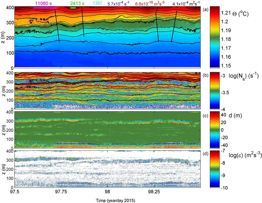
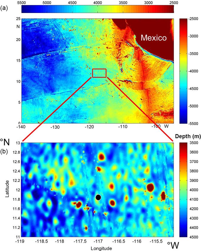
4388                                                         H. van Haren: Abyssal plain hills and internal wave turbulence

However, abyssal plains occupy a large part of the ocean and       intermittent, producing a very step-like, non-smooth, sheet-
the processes that occur there deserve investigation. For ex-      and-layer-structured ocean interior stratification (e.g. Lazier,
ample, hills on the bottom form corrugated topography in-          1973; Fritts et al., 2016). In the near-surface ocean, such in-
stead of the seemingly flat bottom and contribute to inter-        ternal wave propagation and deformation “straining” of strat-
nal wave generation and breaking. These hills are so numer-        ification has been observed to migrate through the density
ous (Baines, 2007; Morozov, 2018) that it may be questioned        field in space and time.
whether the abyssal plain and its overlying waters may be             The lower bound of inertio-gravity wave (IGW) fre-
called a “quiescent zone”.                                         quencies is determined by the local vertical Coriolis pa-
   This is because occasional “benthic storms” have been           rameter, i.e. the inertial frequency, f = 2 sin ϕ, of the
reported to disturb the quiescence, even at great depths           Earth rotational vector  at latitude ϕ. This bound be-
> 5000 m (Hollister and McCave, 1984). The effects can be          comes significantly modified to lower sub-inertial fre-
significant on sediment reworking and particles remain resus-      quencies under weak stratification (∼ N 2 ) when N < 10f .
pended long after the “storm” has passed. Such resuspension        From non-approximated equations, minimum and maximum
has obvious effects on deep-sea benthic biology and reminer-       IGW frequencies are calculated as [σmin , σmax ] = (s ∓ (s 2 −
alization (e.g. Lochte, 1992).                                     f 2 N 2 )1/2 )1/2 using 2s = N 2 + f 2 + fh2 cos2 γ , in which γ is
   In order to avoid semantic problems, the term “benthic          the angle to the north (γ = 0 denotes meridional propaga-
boundary layer” is reserved here for the sediment–water in-        tion) and the horizontal component of the Coriolis parameter
terface (at the bottom of the water phase of the ocean), fol-      fh = 2 cos ϕ becomes important for internal wave dynam-
lowing common practice by sedimentologists and marine              ics (e.g. LeBlond and Mysak, 1978; Gerkema et al., 2008).
chemists (e.g. Boudreau and Jørgensen, 2001). The term                In the present paper, detailed moored observations from
“bottom boundary layer” follows the physical oceanographic         a Pacific abyssal plain confirm the Lazier (1973) sheet-and-
convention to describe the lower part of the water phase of        layer stratification. The new observations are used to inves-
the ocean, which is almost uniform in density, using the           tigate the interplay between motions in the stratified interior
threshold criterion of the large-scale (100 m) buoyancy fre-       and the effects on the bottom boundary layer. The small-scale
quency N < 3 × 10⁻⁴ s−1 . This is the layer of investigation       topography may prove non-negligible for internal waves in
here together with overlying higher density-stratified waters      comparison with large oceanic ridges, seamounts and conti-
in the interior. The amount of homogeneity is also a subject       nental slopes. Following Bell (1975), recent studies demon-
of study. Historic observations have demonstrated the vari-        strate the potential of substantial internal wave generation by
ability of the abyssal plain bottom boundary layer in space        flow over abyssal hills under particular slope and stratifica-
and time (e.g. Wimbush, 1970; Armi and Millard, 1976;              tion conditions (e.g. Nikurashin et al., 2014; Hibiya et al.,
Armi and D’Asaro, 1980).                                           2017). We are interested in the observational details of the
   Similar to the ocean interior, waters above abyssal plains      IGW-induced turbulent processes.
are considered calm ocean regions in terms of weak turbulent
exchange. However, the (bulk) Reynolds number Re = U L/ν
as a measure for the transition from laminar (“molecular”)         2   Methods and data handling
to turbulent flow is not small. With the kinematic viscosity
ν ≈ 1.5 × 10⁻⁶ m2 s−1 to characterize the molecular water          Observations were made from the German R/V Sonne cruises
properties, characteristic velocity U ≈ 0.05 m s−1 and length      SO239 and SO240 above the abyssal hills in the Clarion–
scale L ≈ 30 m of the (internal wave) water flow, Re ≈ 106 ,       Clipperton Fracture Zone of the north-east equatorial Pa-
which is highly turbulent (e.g. Tennekes and Lumley, 1972;         cific Ocean, west of the oriental Pacific Ridge (Fig. 1). The
Fritts et al., 2016) even for the unbounded open-ocean and         data were collected in the German licence area for poly-
atmosphere interiors.                                              metallic nodule exploration. The area is not mountainous
   Both convective instability of the gravitationally unsta-       but also not flat. It is characterized by numerous hills ex-
ble denser over less dense water and shear-induced Kelvin–         tending several hundred metres above the surrounding sea
Helmholtz instability KHi are probable for internal wave           floor. The average bottom slope is 1.2 ± 0.6◦ , computed
breaking; for a recent model see Thorpe (2018). Earlier mod-       from Fig. 1b using the 10 resolution version of the Smith
els (e.g. Garrett and Munk, 1972) suggested KHi was domi-          and Sandwell (1997) sea-floor topography. This slope is
nant over convective instabilities, especially considering the     about 3 times larger than that of the Hatteras Plain (the
construction of the internal wave field of the smallest verti-     area of observations by Armi and D’Asaro, 1980) and
cal scales residing at their lowest frequencies (e.g. LeBlond      about 3 times smaller than that for a similar size area
and Mysak, 1978). Most kinetic energy is found at these fre-       from the Mid-Atlantic Ridge (west of the Azores). Sea-
quencies and thus a large background shear is generated (e.g.      Bird SBE 911plus CTD profiles were collected 1 km around
Alford and Gregg, 2001) through which shorter length-scale         11◦ 50.6300 N, 116◦ 57.9380 W in 4114 ± 20 m of water depth
waves near the buoyancy frequency propagate, break and             on 20–23 March and 6 June 2015. Between 19 March and
overturn. The result is an open-ocean wave field that is highly    2 June a taut-wire mooring was deployed at the above coor-

Biogeosciences, 15, 4387–4403, 2018                                                      www.biogeosciences.net/15/4387/2018/
H. van Haren: Abyssal plain hills and internal wave turbulence                                                                 4389

                                                                     was < 0.02 s and the 400 m profile was measured nearly in-
                                                                     stantaneously. As in the abyssal area temperature variations
                                                                     are extremely small, so severe constraints were put on the de-
                                                                     spiking and noise levels of the data. Under these constraints,
                                                                     35 (17 % of) T sensors showed electronic timing, calibration
                                                                     or noise problems. Their data are no longer considered and
                                                                     are linearly interpolated. This low biases the estimates of tur-
                                                                     bulence parameters like dissipation rate and diffusivity from
                                                                     T-sensor data by about 10 %. Appendix B describes further
                                                                     data processing details.
                                                                        During 3 days around the time of mooring deployment and
                                                                     2 days after recovery, shipborne conductivity–temperature–
                                                                     depth (CTD) profiles were made for the monitoring of the
                                                                     temperature–salinity variability from 5 m below the surface
                                                                     to 10 m a.b. A calibrated CTD was used. The CTD data were
                                                                     processed using the standard procedures incorporated in the
                                                                     SBE software, including corrections for cell thermal mass
                                                                     using the parameter setting of Mensah et al. (2009) and sen-
                                                                     sor time alignment. All other analyses were performed with
                                                                     conservative (∼ potential) temperature (2), absolute salinity
                                                                     (SA) and density anomalies σ4 referenced to 4000 dbar using
                                                                     the GSW software described in IOC et al. (2010).
                                                                        After the establishment of the temperature–density rela-
                                                                     tionship from shipborne CTD profiles (Appendix B), the
                                                                     moored T-sensor data are used to estimate turbulence dis-
                                                                     sipation rate ε = c12 d 2 N 3 and vertical eddy diffusivity Kz =
Figure 1. Bathymetry map of the tropical north-east Pacific based    m1 c12 d 2 N following the method of reordering potentially un-
on the Topo_9.1b 10 version of satellite altimetry-derived data by   stable vertical density profiles in statically stable ones, as
Smith and Sandwell (1997). The black dot in panel (b) indicates      proposed by Thorpe (1977). Here, d denotes the displace-
mooring and CTD positions. Note the different colour ranges be-      ments between unordered (measured) and reordered profiles
tween the panels.                                                    and N is computed from the reordered profiles. We use stan-
                                                                     dard constant values of c1 = 0.8 for the Ozmidov–overturn
                                                                     scale factor and m1 = 0.2 for the mixing efficiency (e.g. Os-
dinates. At this latitude f = 0.299×10⁻⁴ s−1 (≈ 0.4 cpd, cy-         born, 1980; Dillon, 1982; Oakey, 1982). The validity of the
cles per day) and fh = 1.427 × 10⁻⁴ s−1 (≈ 2 cpd). A 130 m           latter is justified after inspection of the temperature-scalar
elevation has its ridge at approximately 5 km west of the            spectral inertial subrange content (being mainly shear driven;
mooring.                                                             compare to Sect. 3) and also considering the generally long
   The mooring consisted of 2700 N of net top buoyancy at            averaging periods over many (> 1000) profiles. The mixing
about 450 m from the bottom. With current speeds of less             efficiency value is close to the tidal mean mixing potential
than 0.15 m s−1 , the buoy did not move more than 0.1 m              observed by Cyr and van Haren (2016), also in layers in
vertically and 1 m horizontally, as was verified using pres-         which stratification is weak. Internal waves not only induce
sure and tilt sensors. The mooring line held three single-           mixing through their breaking but also allow for rapid re-
point Nortek AquaDopp acoustic current meters at 6, 207              stratification, making the mixing rather efficient.
and 408 m a.b. The middle current meter was clamped to a                The moored T-sensor data are thus much more precise
0.0063 m diameter plastic-coated steel cable. To this 400 m          and apt for using Thorpe overturning scales to estimate tur-
long insulated cable 201 custom-made NIOZ4 temperature               bulence parameters than shipborne CTD data. Most of the
sensors were taped at 2.0 m intervals. To deploy the 400 m           concerns raised e.g. by Johnson and Garrett (2004) on this
long instrumented cable it was spooled from a custom-made            method using shipborne CTD data are not relevant here.
large-diameter drum with separate “lanes” for T sensors and          First, instead of a single (CTD) profile, averaging is per-
the cable (Appendix A).                                              formed over 103 –104 profiles, i.e. at least over the buoyancy
   The NIOZ4 T-sensor noise level is < 0.1 mK (verified in           timescale and more commonly over the inertial timescale.
Appendix B), and the precision is < 0.5 mK (van Haren et al.,        Second, the mooring does not move more than 0.1 m verti-
2009; NIOZ4 is an update of NIOZ3 with similar characteris-          cally and if moving it does so on a sub-inertial timescale; no
tics). The sensors sampled at a rate of 1 Hz and were synchro-       corrections are needed for “ship motions” and instrumental
nized via induction every 4 h so that their timing mismatch          and frame flow disturbance, as for CTD data. Third, the noise

www.biogeosciences.net/15/4387/2018/                                                        Biogeosciences, 15, 4387–4403, 2018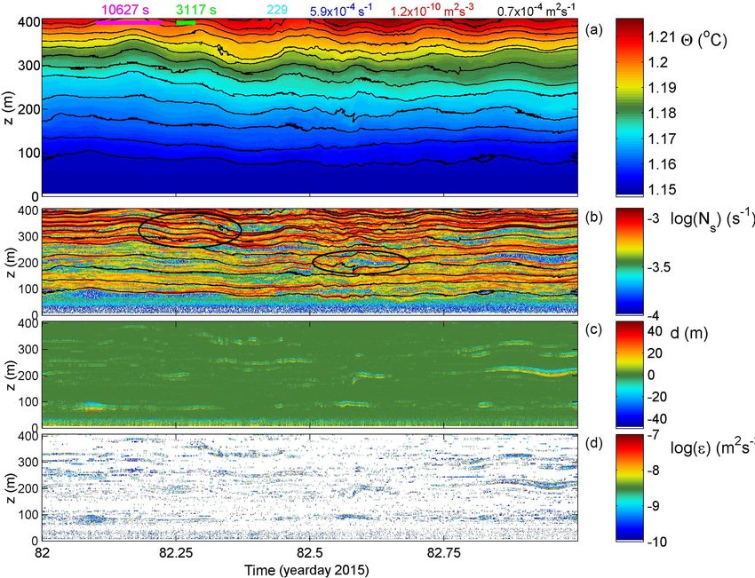
4390                                                           H. van Haren: Abyssal plain hills and internal wave turbulence

level of the moored T sensors is very low, about one-third of           The T sensors have identical instrumental (white) noise
the high-precision sensors used in a Sea-Bird 911 CTD (Ap-           levels at frequencies σ > 104 cpd and near-equal variance
pendix B). Fourth, the environment in which the observations         at sub-inertial frequencies σ < f (Fig. 2c). From the for-
are made is dominated by internal wave breaking (above to-           mer an approximate 1 standard deviation is observed of
pography), in which turbulent mixing is generally not weak           SD ≈ 4 × 10⁻⁵ ◦ C; see also Appendix B. In the frequency
and there is a tight temperature–density relationship. Be-           range in between and especially for f ∼ < σ ∼ < N, the up-
cause of points three and four, complex noise reduction as           per T-sensor data demonstrate the largest variance by up to
in Piera et al. (2002) is not needed for moored T-sensor data.       2 orders of magnitude at σ ≈ N compared with the lower T-
More in general for these data in such environments, Thorpe          sensor data. In this frequency range, the upper T-sensor spec-
overturning scales can be solidly determined using temper-           trum has a slope of about −1 in the log–log domain, which
ature sensor data instead of more imprecise density (T- and          reflects a dominance of smooth quasi-linear ocean interior
S-sensor data), as salinity intrusions are not found important       IGW (van Haren and Gostiaux, 2009). Extending above this
as verified. The buoyancy Reynolds number Reb = ε/νN 2 is            slope is a small near-inertial peak reflecting rarely observed
used to distinguish between areas of weak, Reb < 100, and            low internal wave frequency vertical motions in weakly strat-
strong turbulence.                                                   ified waters (van Haren and Millot, 2005). The steep −3 roll-
   In the following, averaging over time is denoted by [. . . ]      off at super-buoyancy frequencies σ > N is also associated
and averaging over depth range by h. . .i. The specific aver-        with IGW. At frequencies in between and for the lower T-
aging periods and ranges are indicated with the mean values.         sensor data throughout the frequency range, a slope of −5/3
The vertical coordinate z is taken upward from the bottom            is found. This reflects passive scalar turbulence dominated
z = 0. Shear-induced overturns are visually identified as in-        by shear (Tennekes and Lumley, 1972). After sufficient av-
clined S shapes in log(N ) panels, while convection demon-           eraging this passive scalar turbulence is efficient (Mater et
strates more vertical columns (e.g. van Haren and Gostiaux,          al., 2015). At intermediate depth levels and in short fre-
2012; Fritts et al., 2016). It is noted that both types occur si-    quency ranges of the spectral data, slopes vary between −2
multaneously, as columns exhibit secondary shear along the           and −1. Slopes between −5/3 and −1 would point at active
edges and KHi demonstrates convection in the interior core           scalar turbulence of convective mixing (Cimatoribus and van
(Matsumoto and Hoshino, 2004; Li and Li, 2006).                      Haren, 2015), while a slope of −2 reflects fine-structure con-
                                                                     tamination (Phillips, 1971) or a saturated IGW field (Garrett
                                                                     and Munk, 1972).
3     Observations                                                      While the upper T-sensor data contain the most variance
                                                                     and hence the most potential energy in the IGW band, the
High-resolution T-sensor data analysis was difficult because
                                                                     spectrum of estimated turbulence dissipation rate demon-
of the very small temperature ranges and variations of only
                                                                     strates nearly 2 orders of magnitude higher variance for the
a few mK over, especially the lower, 100 m of the observed
                                                                     lowest T-sensor data around σ ≈ f (Fig. 2b). The stratifi-
range. This rate of variation is less than the local adiabatic
                                                                     cation around the upper sensor supports substantial internal
lapse rate. First, a spectral analysis is performed to investi-
                                                                     waves, but weak turbulence provides a flat and featureless
gate the internal wave and turbulence range and slope ap-
                                                                     spectrum of the dissipation rate time series. The lower layer
pearance. Then, particular turbulent overturning aspects of
                                                                     ε spectrum shows a relative peak near σ ≈ 2f besides one
internal wave breaking are demonstrated in magnifications
                                                                     at sub-inertial frequencies, but no peaks at the inertial and
of time–depth series. Finally, profiles of mean turbulence pa-
                                                                     semidiurnal tidal frequencies. The lack of peaks at the lat-
rameter estimates are used to focus on the extent and nature
                                                                     ter frequencies is somewhat unexpected as the kinetic energy
of the bottom boundary layer.
                                                                     (Fig. 2b, blue spectrum) is highly dominated by motions at
3.1    Spectral overview                                             M2 and, to a lesser extent, at just super-inertial 1.04f .
                                                                        In contrast, the “large-scale shear” spectrum computed
The small temperature ranges are reflected in the low val-           between current meters 200 m apart (Fig. 2b, light blue)
ues of the large-scale stratification (Fig. 2a). (Salinity con-      shows a single dominant peak at just sub-inertial 0.99f ,
tributes weakly to density variations; Appendix B.) Typical          with a complete absence of a tidal peak. This reflects large
buoyancy periods are 3 h, increasing to roughly 9 h in near-         quasi-barotropic vertical length scales > 400 m exceeding
homogeneous layers, e.g. near the bottom. In spite of the            the mooring range at semidiurnal tidal frequencies and com-
weak stratification, the IGW band approximately between              monly known “small” ≤ 200 m vertical length scales at
and including f and N is 1 order of magnitude wide. This             near-inertial frequencies. The large-scale shear has an av-
IGW bandwidth is observable in spectra of turbulence dissi-          erage magnitude of h|S|i = 2 × 10⁻⁴ s−1 for 207–408 m a.b.
pation rate (Fig. 2b) and temperature variance (Fig. 2c).            and 1.6 × 10⁻⁴ s−1 for 6–207 m a.b., with peak values of
                                                                     |S| = 6 × 10⁻⁴ s−1 and 4 × 10⁻⁴ s−1 , respectively. Consid-
                                                                     ering mean hNi ≈ 5.5 × 10⁻⁴ s−1 with variations over 1 or-
                                                                     der of magnitude, the mean gradient Richardson number

Biogeosciences, 15, 4387–4403, 2018                                                      www.biogeosciences.net/15/4387/2018/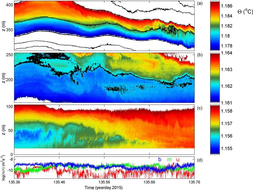
H. van Haren: Abyssal plain hills and internal wave turbulence 4391
Figure 2. Stratification and spectral overview. (a) Vertical profiles of buoyancy frequency scaled with the local horizontal component of the
Coriolis parameter fh and smoothed over 50 dbar (∼ 50 m) from all five CTD stations to within 1 km from the mooring. The blue, green
and red profiles are made around the time of mooring deployment. (b) Weakly smoothed (10 degrees of freedom, DOF) spectra of kinetic
energy (upper current meter; green) and current difference (between upper and middle current meters; light blue). In red and purple are
the spectra of 150 s subsampled time series of 100 m vertically averaged turbulence dissipation rates for the lower (7–107 m a.b.) and upper
(307–407 m a.b.) T-sensor data segments, respectively. The inertial frequency f , fh including several higher harmonics, buoyancy frequency
N including range and the semidiurnal lunar tidal frequency M2 are indicated. Nmax indicates the maximum small-scale buoyancy frequency.
(c) Weakly smoothed (10 DOF) spectra of 2 s subsampled temperature data from three heights representing upper, middle and lower levels.
For reference, several slopes with frequency are indicated.
Ri = N 2 /|S|2 is larger than unity, while marginally stable about 15 m, the stratification is organized in fine-scale layer-
conditions (Ri ≈ 0.5; Abarbanel et al., 1984) occur regu- ing throughout, except for the lower 50 m of the range. De-
larly in “bursts”. Unfortunately, higher-vertical-resolution tailed inspection of sheets (large values of small-scale Ns
acoustic profiler current measurements were not available in Fig. 3b) demonstrates that they gain and lose strength
to establish smaller-scale shear variations associated with “strain” over timescales of the buoyancy period and shorter
higher-frequency internal waves propagating through the and that they merge and deviate (e.g. around 300 m a.b. be-
(large-scale) shear generated by near-inertial motions. Such tween days 82.25 and 82.5 in Fig. 3b; upper left black el-
smaller-scale variations in shear are expected in association lipse) also from the isotherms in association with the largest
with sheet-and-layer variation in stratification observed using turbulent overturns (Fig. 3c) eroding them. This is reflected
the detailed high-resolution T sensors. in non-smooth isotherms (e.g. the interior overturning near
220 m a.b. and day 82.6 in Fig. 3b; right ellipse). The patches
3.2 Detailed periods of interior turbulent overturns, with displacements |d| < 10 m
in this example, are elongated in time–depth space, having
timescales of up to the local buoyancy period but not longer.
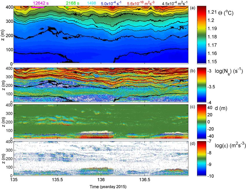
The days shortly after deployment were amongst the qui-
Thus, it is unlikely they represent an intrusion that can have
etest in terms of turbulence during the entire mooring
timescales (well) exceeding the local buoyancy timescale.
period. Nevertheless, some near-bottom and interior tur-
Considering the 0.05 m s−1 average (tidal) advection speed,
bulent overturning was observed occasionally (Fig. 3).
their horizontal spatial extent is estimated to be about 500 m.
For this example, averages of turbulence parameters
This extent is very close to the estimated baroclinic “internal”
for a 1-day time interval and 400 m vertical inter-
Rossby radius of deformation Roi = N H /nπf ≈ 600 m for
val are estimated as [hεi] = 1.2 ± 0.8 × 10⁻¹⁰ m2 s−3 and
vertical length scale H = 100 m and first mode n = 1.
[hKz i] = 7 ± 4 × 10⁻⁵ m2 s−1 . These values are typical for
The near-bottom range is different, with buoyancy periods
open-ocean “weak turbulence” conditions although mean
approaching the semidiurnal period and sometimes longer.
Reb ≈ 200. The shortest isotherm distances are observed far
However, a permanent turbulent and homogeneous bottom
above the bottom (a few hundred metres; Fig. 3a), reflecting
boundary layer is not observed after further detailing (Fig. 4).
the generally stronger stratification (Fig. 3b) there. While the
Examples of the upper, middle and lower 100 m of the
upper isotherms smoothly oscillate with a periodicity close
T-sensor range are presented in magnifications with differ-
to the average buoyancy period of 3.2 h and amplitudes of
www.biogeosciences.net/15/4387/2018/ Biogeosciences, 15, 4387–4403, 2018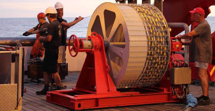
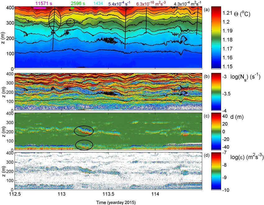
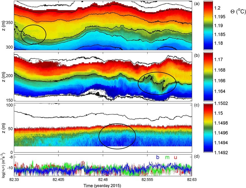
4392                                                              H. van Haren: Abyssal plain hills and internal wave turbulence

Figure 3. A 1-day sample detail of moored temperature observations during relatively calm conditions (on the day of calibration in the
beginning of the record). (a) Conservative temperature. The black contour lines are drawn every 0.005 ◦ C. At the top from left to right are
two time references indicating the mean (purple bar) and shortest (green bar) buoyancy periods found in this data detail. Values for time–
depth–range–mean parameters are given by the buoyancy Reynolds number (light blue), buoyancy frequency (blue), turbulence dissipation
rate (red) and turbulent eddy diffusivity (black). Errors for the latter two are to approximately within a factor of 2. (b) Logarithm of small-
scale (2 dbar) buoyancy frequency from reordered temperature profiles. The black isotherms are reproduced from panel (a). (c) Thorpe
displacements between raw (a) and reordered T profiles. (d) Logarithm of turbulence dissipation rate.

ent colour ranges while maintaining the same isotherm in-                 is quasi-permanently in turbulent overturning but in specific
terval of 5 mK (Fig. 4a–c). For this period, the mean flow is             bands only around 310 m a.b. and around 160 m a.b. (Fig. 5c,
0.04 ± 0.01 m s−1 towards the SE, more or less off slope of               d). The latter is approximately the height of the nearest crest,
the small ridge located 5 km west of the mooring. Between                 still 5 km away from the mooring. RMS vertical overturn
these panels, the high-frequency internal wave variations de-             displacements are 2–3 times larger than in the previous ex-
crease in frequency from upper to lower, but all panels do                ample. Their duration is commensurate with the local buoy-
show overturning (e.g. as indicated by the black ellipses                 ancy periods. The smooth upper range isotherms centred
(around 330 m a.b. and day 82.35 in Fig. 4a, 200 m a.b. and               around 360 m a.b. are reflected in a 75 m, 1-day-wide range
day 82.6 in Fig. 4b, and 35 m a.b. and day 82.5 in Fig. 4c). In           of turbulence dissipation rates below threshold (Fig. 5d).
Fig. 4c the entire T colour range represents only 1 mK. In this           But, above and especially below, turbulent overturning is
depth range, the low-frequency variation in temperature and,              more intense; see also the detailed panels (Fig. 6). While
while not related, stratification vary with a period of about             shear-induced overturning is seen (e.g. in the black ellipses
15.5 h. These variations do not have tidal-harmonic period-               around 350 m a.b. day 98.0 (Fig. 6a) and around 200 m a.b.
icity and thus do not reflect bottom friction of the dominant             day 97.95; Fig. 6b), convective turbulence columns are ob-
tidal currents. Quasi-convective overturning seems to occur               served (e.g. around 60 m a.b. and day 98; Fig. 6c, black el-
after day 82.5. In the interior > 100 m a.b. most overturning             lipse). It is noted, however, that in the presented data we
seems shear induced.                                                      cannot distinguish the fine-detailed secondary overturning,
   The overturning phenomena are more intensely observed                  e.g. shear-induced billow formation, on convection “verti-
during a less quiescent day (Figs. 5, 6) when turbulence val-             cal columns”. In the lower 100 m a.b., overturning occurs
ues are about 5 times larger and mean Reb ≈ 1400. Between                 on large (∼ 50 m, hours) scales but also on much shorter
300 and 400 m a.b. isotherms remain quite smooth with near-               timescales of 10 min. This results in isotherm excursions
linear internal wave oscillations (Fig. 5a, b). The lower 300 m           that are faster than further away from the bottom. A cou-

Biogeosciences, 15, 4387–4403, 2018                                                             www.biogeosciences.net/15/4387/2018/
H. van Haren: Abyssal plain hills and internal wave turbulence                                                                         4393

Figure 4. Magnifications of Fig. 3a using different colour ranges but maintaining the 5 mK distance between isotherms. (a) Upper 100 m
of the temperature sensor range (T range). (b) Approximately the middle 100 m of the T range. (c) Bottom 100 m of the T range; note the
entire colour range extending over 1 mK only. (d) Time series of the logarithm of vertical mean turbulence dissipation rates from Fig. 3d for
panels (a), (b) and (c) labelled u, m and b, respectively.

Figure 5. As Fig. 3 with identical colour ranges, but for a 1-day period with more intense turbulence, especially near the bottom.

www.biogeosciences.net/15/4387/2018/                                                              Biogeosciences, 15, 4387–4403, 2018
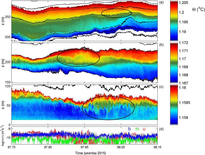
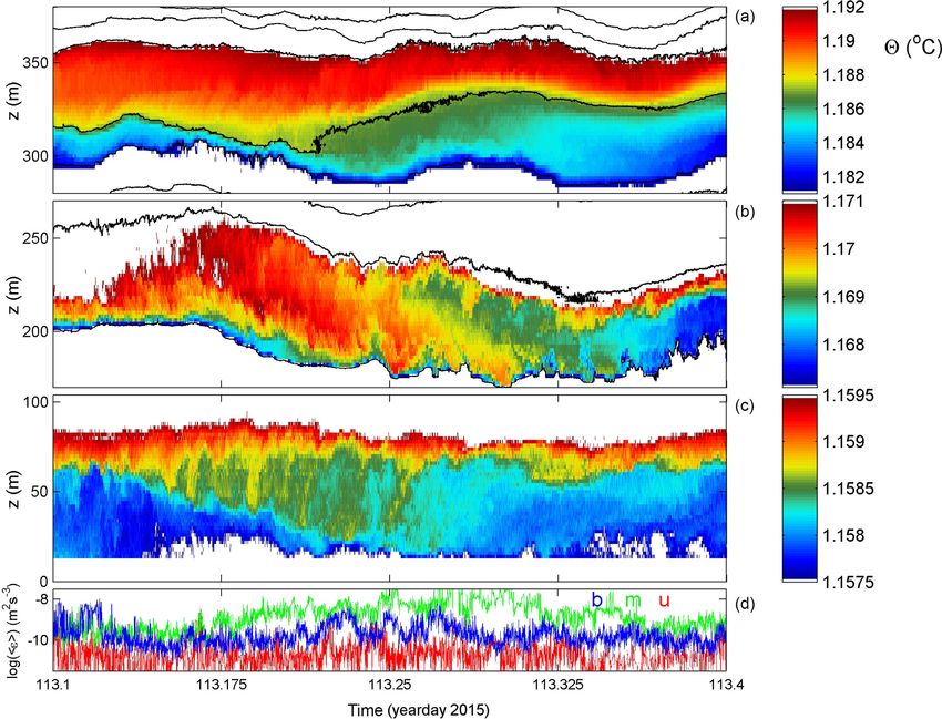
4394                                                              H. van Haren: Abyssal plain hills and internal wave turbulence

Figure 6. As Fig. 4, but associated with Fig. 5 and using different colour ranges.

pling between interior and near-bottom (turbulence and in-                50 m near 200 m a.b. (Fig. 8b). This slanting layer of elon-
ternal wave) motions is difficult to establish. For example,              gated overturns seems originally shear induced, but the over-
short-scale (high-frequency σ  f ) internal wave propaga-                turns show clear convective properties during the observed
tion > 200 m a.b. shows a downward phase (i.e. upward en-                 stage. The largest duration of patches is close to the lo-
ergy) propagation around day 97.75 (Fig. 5a) with no clear                cal mean buoyancy period. The entire layer demonstrates
correspondence with the lower 100 m a.b. Between days 98.2                numerous shorter-timescale overturning. Crossovers, sudden
and 98.5, however, the phase propagation appears upward                   changes in the vertical, are observed in isotherms from thin
(downward energy propagation), with some indication for                   high-Ns above low-Ns turbulent patches to below the low-
correspondence between the upper 200–400 m a.b. and lower                 Ns patches, e.g. day 112.6 in Fig. 7b and vice versa, e.g.
100 m a.b. During this period the mean 0.04 m s−1 flow was                days 113.1 and 113.5. (Recall that small-scale Ns is com-
towards the west (upslope).                                               puted from reordered 2 profiles.) This evidences one-sided,
   Another example (of 2 days) of rather intense turbu-                   rather than two-sided, turbulent mixing eroding a stratified
lence is given in Figs. 7 and 8, with similar average val-                layer either from below or above.
ues as in the previous example. It demonstrates in partic-                   The interior shear-induced turbulent overturning seems to
ular relatively large-amplitude near-N internal waves (e.g.               have some correspondence with the (top of) the near-bottom
day 112.9, 310 m a.b.; Fig. 7a, left black ellipse) and bursts            layer: on days 113.1–113.6 interior mixing is accompanied
of elongated weakly sloping (slanting) shear-induced over-                by similar near-bottom mixing. The status of the near-bottom
turning (e.g. day 113.2, 210 and 50 m a.b.; Fig. 7c, black                layer (z < 75 m a.b.) switches from large-scale convective in-
ellipses). The near-N waves appear quasi-solitary, lasting a              stabilities (day < 113.1) to stratified shear-induced overturn-
maximum of two periods and having about 30 m trough–                      ing (113.1 < day < 113.6) and back to large-scale convection
crest level variation. As before, the vertical phase propaga-             with probably secondary shear instabilities (day > 113.6).
tion of these waves is ambiguous. In addition, very high-                 This is visible in the displacements (Fig. 7c) and dissipation
frequency “internal waves” around the small-scale buoyancy                rate (Fig. 7d), and part of it is visible in detailed temper-
frequency are observed in the present example, with small                 ature (Fig. 8c). The transitions between near-bottom “mix-
amplitudes < 10 m visible in the isotherms around 300 m a.b.              ing regimes” are abruptly marked by near-bottom fronts. The
on day 113.1 (Fig. 7a, right black ellipse).                              mean 0.03 m s−1 flow is south-west directed (more or less on
   The interior turbulent overturning appears more intense                slope).
than in preceding examples, with larger excursions of about

Biogeosciences, 15, 4387–4403, 2018                                                           www.biogeosciences.net/15/4387/2018/
H. van Haren: Abyssal plain hills and internal wave turbulence                                                                  4395

Figure 7. As Fig. 3 with identical colour ranges, but for a 2-day period with occasional long shear turbulence.

Figure 8. As Fig. 4, but associated with Fig. 7 and using different colour ranges.

www.biogeosciences.net/15/4387/2018/                                                              Biogeosciences, 15, 4387–4403, 2018
4396                                                             H. van Haren: Abyssal plain hills and internal wave turbulence

Figure 9. As Fig. 3 with identical colour ranges, but for a 2-day period with some intense convective turbulence also near the bottom.

   A 2-day example of a relatively intensely turbulent near-            lead to some counter-intuitive averaging of displacement val-
bottom layer is given in Figs. 9 and 10. Two periods about 9 h          ues greater than the local distance to the bottom at particular
long (around days 135.9 and 136.8) and 22 h apart demon-                depths. However, it is noted that Prandtl’s concept of overturn
strate > 50 m tall convective overturning extending nearly              sizes never exceeding the distance to a solid boundary was
100 m a.b. In between, large-scale shear-induced overturning            based on turbulent friction of flow over a flat plate. As Ten-
dominates, with a possible correspondence with the interior             nekes and Lumley (1972) indicate, such “mixing length the-
in the form of a large-scale doming of isotherms and mixing             oretical concept” may not be valid for flows with more than
in patches around day 135.4 (lasting 135.25 < day < 135.75,             one characteristic velocity. The present area is not known
generally around 200 m a.b.). The doming interior isotherms             for geothermal fluxes, which are also not observed in the
are not repeated in the lowermost isotherm capping of the               present data. Here, the dominant turbulence generation pro-
near-bottom layer, except perhaps for the down-going flank              cess seems to be induced by internal waves, as the observed
or front. The mean north-east flow is 0.03 m s−1 and directed           turbulence extends well above the layer (of the order of 10 m)
more or less off slope. In this example as well as in previous          of bottom friction.
ones no evidence is found for “smooth” intrusions, as demon-               The mean dissipation rate (Fig. 11a) and diffusivity
strated in the atmospheric DNS model by Fritts et al. (2016).           (Fig. 11b) profiles are observed to be largest between 7 and
                                                                        60 m a.b., with values at least 10 times higher than in the inte-
3.3    Mean profiles                                                    rior. This suggests an internal wave breaking impact on sedi-
                                                                        ment resuspension. Near the bottom, stratification (Fig. 11c)
The different mixing observed in the interior and near the              is low but not as weak as some 15 m higher up. At about
bottom is reflected in the “mean profiles” of estimated tur-            30 m a.b. local minima of [ε] and [Kz ] are found. The av-
bulence parameters (Fig. 11a–c). These plots are constructed            erage top of the weakly stratified N < 3 × 10⁻⁴ s−1 ≈ 4 cpd
from patching together consecutive 1-day portions of data               “bottom boundary layer” is at about 65 m a.b. (Fig. 11d).
that are locally drift-corrected. Time-averaged values of [ε],          This sub-maximum in the PDF distribution is broader than
turbulent flux (providing average [Kz ]) and stratification             a second maximum closer to the bottom, near 10 m a.b. This
(providing average [N]) are computed for each depth level.              smaller bottom boundary layer is probably induced by cur-
Averaging over a day and longer exceeds the buoyancy pe-                rent friction, whereas the larger layer with an average of
riod even in these weakly stratified waters. It is thus consid-         65 m a.b. is probably induced by internal wave turbulence.
ered appropriate for internal-wave-induced mixing. This may             Around 110 m a.b. the maximum of the bottom boundary

Biogeosciences, 15, 4387–4403, 2018                                                            www.biogeosciences.net/15/4387/2018/
H. van Haren: Abyssal plain hills and internal wave turbulence 4397
Figure 10. As Fig. 4, but associated with Fig. 9 and using different colour ranges.
layer is found with few occurrences (Fig. 11d). Around that of the mooring is well outside the baroclinic Rossby radius
height, the profile minimum turbulence values are observed of deformation (Roi ≈ 500 m). It is not likely to influence the
at the depth of a weak local maximum N (Fig. 11c). This near-bottom turbulence here, also because no correlation is
layer separates the interior turbulent mixing with a maximum found between across-slope flow and turbulence intensity.
around 200 m a.b. and the “near-bottom” (< 100 m a.b.) mix- The interior is occasionally found quiescent, with parame-
ing. From the detailed data in Sect. 3.2 correspondence is ob- ter values below the threshold of very weak turbulence at
served between these layers, occurring at least occasionally. about 10 times molecular diffusion values. More commonly
Considering the weaker (mean) turbulence in between, it is the interior is found weakly to moderately turbulent with
expected that the correspondence is communicated via inter- values commensurate with open-ocean values (e.g. Gregg,
nal waves and their shear. As for freely propagating IGW, 1989) following the interaction of high-frequency internal
its frequency band has a 1 order of magnitude width nearly wave breaking and inertial shear.
everywhere, also close to the bottom (Fig. 11c). It is noted The observed dominance of near-inertial shear at the
that inertial waves from all (horizontal) angles can propagate 200 m vertical scale, the vertical separation distance between
through homogeneous, weakly and strongly stratified layers, the current meters, is found far below the depths of atmo-
thus providing local shear (LeBlond and Mysak, 1978; van spheric disturbance generation near the surface. It seems re-
Haren and Millot, 2004). lated to local generation, possibly in association with the
hilly topography (St. Laurent et al., 2012; Nikurashin et al.,
2014; Alford et al., 2017; Hibiya et al., 2017). Also, the
4 Discussion 200 m vertical scale is observed to far exceed the excursion
length (amplitude) of the internal waves, the scale of over-
The observed turbulence at 100 m and higher above the sea turn displacements and the size of most density stratification
floor is mainly induced by (sub-)inertial shear and (small- layering. In contrast, above the Mid-Atlantic Ridge where
scale) internal wave breaking. This confirms suggestions by tidal currents are only twice as energetic as near-inertial mo-
Garrett and Munk (1972) about interior IGW. However, this tions, the vertical length scale of tides equals that of near-
shear is not found to decrease with N (depth) in the present inertial motions around 100–150 m (van Haren, 2007). There
data. The > 100 m a.b. depth range is termed “the interior” and in the open ocean, near-inertial motions dominate shear
here, although perhaps it is not representative of the “mid- at shorter scales with an expected peak around 25 m (e.g.
water ocean” as it is still within the height range of the sur- Gregg, 1989). Like in the present data, the near-inertial shear
rounding hilly topography. The 130 m high ridge 5 km west
www.biogeosciences.net/15/4387/2018/ Biogeosciences, 15, 4387–4403, 20184398 H. van Haren: Abyssal plain hills and internal wave turbulence Figure 11. Profiles of turbulence parameters from entire-record time-averaged estimates using 1-day drift-corrected, 150 s subsampled moored temperature data. (a) Logarithm of dissipation rate. (b) Logarithm of eddy diffusivity. (c) Logarithm of small-scale (2 dbar) buoyancy frequency from the T sensors (black) for comparison with the mean of the five CTD profiles smoothed over 50 dbar vertical intervals from Fig. 2a (red). The green dashed curves indicate the minimum (to the left of the f line) and maximum (to the right of the N profile) inertio- gravity wave bounds for meridional internal wave propagation (see text). (d) Probability density function (PDF) of the “bottom boundary layer height”, the level of the first passage of threshold N > 3 × 10⁻⁴ s−1 , indicating the stratification capping the “near-homogeneous” layer from the bottom upward. Two peaks are visible, one near 10 m a.b. attributable to bottom friction and another around 65 m a.b. attributable to internal-wave-induced turbulence. showed a shift to sub-inertial frequencies (van Haren, 2007). although parameterizations provide 1 order of magnitude Because the shear magnitude was found to be concentrated differences: δ = (2A/f )1/2 , with A the turbulent viscosity in sheets of high N, it was suggested that this red shift was if A = Kz ≈ 10−4 –10−3 m2 s−1 (Fig. 11b), δ ≈ 2.5–8 m or due to the broadening of the IGW band in low-N layers. As a δ = 2 × 10⁻³ U/f ; U ≈ 0.05 m s−1 , δ ≈ 30 m (e.g. Tennekes result, an effective coupling between shear, stratification and and Lumley, 1972). Both are (substantially) less than the the IGW band was established. Considering the similarity in NBTZ found here, which thus seems to be governed by other sheet and layering and (large-scale) shear, such coupling is processes such as IGW breaking. Such a relatively weak con- also suggested in the present observations from the deep sea tribution of bottom friction compared to interior shear and over less dramatic topography. internal wave turbulence was also observed using the in- As for a potential coupling between the interior and the strumentation near the bottom of throughflows like the Ro- observed more intense near-bottom turbulence, internal wave manche Fracture Zone (van Haren et al., 2014) and Kane Gap propagation is found in both the up and down directions. In (van Haren et al., 2013) where current speeds are larger than the lower 50 m a.b. the variability in turbulence intensity, in ∼ 0.25 m s−1 . The throughflow data form a contrast with the turbulence processes of shear and convection, and in strati- present observations because the near-bottom zone is strati- fication demonstrates a non-smooth bottom boundary layer, fied there despite relatively strong shear flow. They are sim- perhaps better defined as an active near-bottom turbulent ilar in showing internal wave convection occasionally pene- zone or NBTZ. As reported by Armi and D’Asaro (1980), trating close to the bottom. the extent above the bottom of turbulent mixing and a near- Sloping fronts are observed near the bottom in Armi and homogeneous mixed layer varies between < 7 and 100 m a.b. D’Asaro (1980), Thorpe (1983) and the present data. How- with a mean of about 65 m a.b. This mean value exceeds the ever, the isopycnal transport of mixed waters seems not common frictional boundary scales that can be computed for to be away from the boundary as proposed in Armi and flow over flat bottoms on a rotating sphere (Ekman, 1905), D’Asaro (1980) but rather into the NBTZ sloping downward Biogeosciences, 15, 4387–4403, 2018 www.biogeosciences.net/15/4387/2018/
H. van Haren: Abyssal plain hills and internal wave turbulence                                                                 4399

with time (present data). This governs the variable height of       5   Conclusions
the NBTZ.
   Although bottom slopes were about 3 times larger in              From the present high-resolution temperature sensor data
the north-east Pacific than above the Hatteras Plain, the           moored up to 400 m above a hilly abyssal plain in the
present observations show many similarities as in Armi and          north-eastern Pacific we find an interaction between small-
D’Asaro (1980). They also show many similarities with               scale internal wave propagation, large-scale near-inertial
equivalent turbulence estimates in both the interior and in         shear and the near-bottom water phase. In an environment
the variable lower 100 m a.b. compared with those from              where semidiurnal tidal currents dominate, 200 m shear is
above the central Alboran Sea, a basin of the Mediter-              the largest at the inertial frequency and near-bottom turbu-
ranean Sea (van Haren, 2015), and with observations                 lence dissipation rates are the largest at twice the inertial
made in the south-east Pacific abyssal hill plains around           frequency. Due to internal wave propagation and occasional
−7◦ 7.2130 S, −88◦ 24.2020 W, east of the oriental Pacific          breaking, stratification in the overlying waters is organized
Ridge (Hans van Haren, unpublished data). Thus it seems             in thin sheets, with less stratified waters in larger layers in
that the precise characteristics (slopes and heights) of the        between, but turbulent erosion occurs asymmetrically. The
hilly topography are not very relevant for the observed in-         average amount of turbulent overturns due to internal wave
ternal wave intensity and turbulence generation as long as          breaking here and there is equal to open-ocean turbulence,
the bottom is not a flat plate and the hills have IGW scales.       with intensities about 100 times larger than those of molec-
This is associated with the suggestion by Baines (2007) and         ular diffusion. The high-frequency internal waves propagate
Morozov (2018) that small-scale topography may prove non-           to near the bottom and likely trigger 10 times larger turbu-
negligible for internal wave generation and dissipation in          lence there as shown in time-averaged vertical profiles. The
comparison with large oceanic ridges, seamounts and conti-          result is a highly variable near-bottom turbulent zone, which
nental slopes. After all, flat bottoms hardly exist in the ocean,   may be near homogeneous over heights of less than 7 and up
depending on the length scale investigated.                         to 100 m above the bottom. This near-bottom turbulence is
   The 10-fold larger turbulence intensity observed here in         not predominantly governed by frictional flows on a rotating
the NBTZ compared to the stratified interior marks a rela-          sphere as in Ekman dynamics that occupy a shorter range
tively extended inertial subrange. Although the near-bottom         (of the order of 10 m) above the bottom. Fronts occur, as
(6 m a.b.) current speeds are typically 0.05 m s−1 up to about      do sudden isotherm uplifts by solitary internal waves. Turbu-
0.10 m s−1 , the estimated turbulence intensity of 103 –104         lence seems shear dominated, but occurs in parallel with con-
times larger than molecular diffusion is sufficient to mix ma-      vection. The shear is quasi-permanent because the dominant
terials up to 100 m a.b., the extent of observed vertical mixing    near-circular inertial motions have a constant magnitude. It is
in the layer adjacent to the bottom. This reflects previous ob-     expected that inertial shear also dominates on shorter scales,
servations of nephels, turbid waters of enhanced suspended          which was not verifiable with the present current meter data,
materials (Armi and D’Asaro, 1980). It is expected that this        possibly added by smaller internal wave shear. In terms of
material is resuspended locally, as the more intensely turbu-       the mean, turbulence dissipation rates exceed the level of
lent, steeper large-scale slopes are too far away horizontally,     10−11 m2 s−3 , except for a 30 m thick layer around 100 m a.b.
far beyond the baroclinic Rossby radius of deformation.             Given the numerous hills distributed over the ocean floor, the
   For the future, modelling may provide better insights into       present observations lend some support to their importance
the precise coupling between near-inertial shear and inter-         for internal wave turbulence generation in the ocean.
nal wave breaking, leading to a combination of convective
and shear-induced overturning. It is expected that interaction
between the semidiurnal tidal current and the hilly topog-          Data availability. Current     meter     and       CTD      data
raphy may generate internal waves near the buoyancy fre-            are stored in the WDC database, PANGAEA, at
                                                                    https://doi.org/10.1594/PANGAEA.891476 (van Haren, 2018). The
quency (Hibiya et al., 2017), while it remains to be investi-
                                                                    moored temperature sensor data are made available upon request to
gated whether the inertial motions and shear are topograph-
                                                                    the author as they need to be computed from the raw data set for
ically or atmospherically driven. The one-sided shear across        any given specific period.
thin-layer stratification, as inferred from observed deviation
of high-N sheets from isotherms and associated with the ver-
tical propagation direction of internal waves, may prove im-
portant for wave breaking.

www.biogeosciences.net/15/4387/2018/                                                       Biogeosciences, 15, 4387–4403, 2018
4400 H. van Haren: Abyssal plain hills and internal wave turbulence
Appendix A: Thermistor string drum: a dedicated Appendix B: Temperature sensor data processing in
instrumented cable spool weakly stratified waters
The deployment of a 1-D T-sensor mooring, a thermistor High-resolution T sensors can be used to estimate verti-
string, is most commonly done for oceanographic moorings. cal turbulent exchange across density-stratified waters un-
Through the aft A frame, the top buoy is put first in the water der particular constraints that are more difficult to account
whilst the ship is slowly steaming forward. The thermistor for under weakly stratified conditions of N < 0.1f . As in
string is coupled between a buoy or other instrument(s) and the present data the full temperature range is only 0.05◦ C
other instrument(s) or acoustic releases before attaching the over 400 m, and careful calibration is needed to resolve tem-
weight that is dropped in free fall. The thermistor string is peratures well below the 1 mK level, at least in relative
put overboard through a wide, relatively large (> ∼ 0.4 m) precision. Correction for instrumental electronic drift of 1–
diameter pulley about 2 m above deck or, preferably, via a 2 mK mo−1 requires shipborne high-precision CTD knowl-
smoothly rounded gunwhale (Fig. A1). Up to a 100 m length edge of the local conditions and uses the physical condition
of string typically holding 100 T sensors can be put over- of static stability of the ocean at timescales longer than the
board manually by one or two people. In that case, the string buoyancy scale (longer than the largest turbulent overturning
is laid on deck in neat long loops. The deployment of a longer timescale). CTD knowledge is also needed to use tempera-
length of string becomes more difficult because of the weight ture data as a tracer for density variations.
and drag. For such strings a 1.48 m inner diameter (1.60 m The NIOZ4 T-sensor noise level is nominally
OD) 1400-pin drum is constructed to safely and fully control < 1 × 10⁻⁴ ◦ C (van Haren et al., 2009; NIOZ4 is an
their overboard operation (Fig. A1). The drum dimensions fit update of NIOZ3 with similar characteristics) and thus po-
in a sea container for easy transportation. The 0.04 m high tentially of sufficient precision. A custom-made laboratory
metal pins guide the cables and separate them from the T tank can hold up to 200 T sensors for calibration against
sensors in “lanes”, while allowing the cables to switch be- an SBE35 Deep Ocean Standards high-precision platinum
tween lanes. The pins are screwed and welded in rows 0.027 thermometer to an accuracy of 2 × 10⁻⁴ ◦ C over ranges of
and 0.023 m apart, the former sufficiently wide to hold the about 25 ◦ C in the domain of [−4, +35] ◦ C. Due to drift
sensors. Up to 18 T sensors can be located in one lane before in the NTC resistors and other electronics of the T sensors,
the next lane is filled. The drum has 14 double lanes and can such accuracy can be maintained for a period of about
store about 230 T sensors and 450 m of cable in one layer. 4 weeks after ageing. However, this period is generally
The longest string deployed successfully thus far held 300 shorter than the mooring period (of up to 1.5 years). During
T sensors and was 600 m long, with about one-quarter of post-processing, sensor drifts are corrected by subtracting
the string doubled on the drum. The doubling did not pose constant deviations from a smooth profile over the entire
a problem, and the sensors were thus well separated so that vertical range and averaged over typical periods of 4–7 days.
entanglement did not occur. For recovery or deployment of Such averaging periods need to be at least longer than the
strings holding up to 150 T sensors, a smooth surface drum buoyancy period to guarantee that the water column is stably
is used of the same dimensions but without pins. stratified by definition (in the absence of geothermal heating
as in the present area). Conservatively, they are generally
taken longer than the local inertial period (here 2.5 days).
In weakly stratified waters as in the present observations,
the effect of drift is relatively so large that the smooth
polynomial is additionally forced to the smoothed CTD
profile obtained during the overlapping time period of data
collection (Fig. B1a). In the present case, this can only be
done during the first few days of deployment. Corrections
for drift during other periods are made by adapting the
local smooth polynomial with the difference of the (smooth
average) CTD profile and the smooth polynomial of the first
few days of deployment. The instrumental noise level can
Figure A1. Photo of thermistor string deployment using the instru- be verified from spectra like in Fig. 2c and, alternatively,
mented cable spooling drum onboard R/V Sonne. from a near-homogeneous period and layer, here between
15 and 50 m a.b. for 1.5 h (Fig. B1b). Its standard deviation
is 4 × 10⁻⁵ ◦ C, which is about one-third of the standard
deviation of the Sea-Bird 911 CTD–T sensor (Johnson and
Garrett, 2004). The calibrated and drift-corrected T-sensor
data are transferred to conservative (∼ potential) temperature
(2) values (IOC et al., 2010) before they are used as a tracer
Biogeosciences, 15, 4387–4403, 2018 www.biogeosciences.net/15/4387/2018/H. van Haren: Abyssal plain hills and internal wave turbulence 4401 for potential density variations δσ4 referenced to 4000 dbar, apparent thermal expansion coefficient is α = δσ4 /δ2 = following the constant linear relationship obtained from −0.223 ± 0.005 kg m−3 ◦ C−1 (n = 5). The resolvable turbu- best-fit data using all nearby CTD profiles over the mooring lence dissipation rate threshold averaged over a 100 m verti- period and across the lower 400 m (Fig. B2). As temperature cal range is approximately 3 × 10⁻¹² m2 s−3 . dominates density variations, this relationship’s slope or Figure B1. Conservative temperature profiles with depth over the lower 400 m a.b. (a) 1-day mean moored sensor data, raw data after calibration (thin black line, yellow filled) and smooth high-order polynomial fit (thick black solid line). In red are three CTD profiles within 1 km from the mooring during the first days of deployment (two solid profiles on day 80–81 coincide in time with moored data mean), and in blue dashed are two CTD profiles after recovery of the mooring. The mean of the two solid red profiles is given by the red dashed-dot profile, 0.015◦ offset for clarity, with its smooth high-order polynomial fit in light blue to which the moored data are corrected. (b) Standard deviation of 1.5 h T-sensor data between days 80.26 and 80.32 when the layer between about 15 and 50 m a.b. is nearly homogeneous. The sensor noise level is indicated by the purple line. Figure B2. Lower 400 m of five CTD profiles obtained near the T-sensor mooring. Red data are from around the beginning of the moored period, blue are from after recovery. (a) Conservative temperature. (b) Absolute salinity with x axis range matching the one in (a) in terms of equivalent relative contributions to density variations. The noise level is larger than for temperature. (c) Density anomaly referenced to 4000 dbar. (d) Density anomaly–conservative temperature relationship (δσ4 = αδ2). The data yielding two representative slopes after linear fit are indicated (the mean of five profiles gives < α > = −0.223 ± 0.005 kg m−3 ◦ C−1 ). www.biogeosciences.net/15/4387/2018/ Biogeosciences, 15, 4387–4403, 2018
You can also read