Detection of repeating earthquakes and their application in characterizing slow fault slip - Progress in Earth and Planetary Science
←
→
Page content transcription
If your browser does not render page correctly, please read the page content below
Uchida Progress in Earth and Planetary Science           (2019) 6:40
https://doi.org/10.1186/s40645-019-0284-z
                                                                                                                              Progress in Earth and
                                                                                                                                 Planetary Science

 REVIEW                                                                                                                                        Open Access

Detection of repeating earthquakes and
their application in characterizing slow fault
slip
Naoki Uchida

  Abstract
  Repeating earthquakes (repeaters) that rupture the same fault area (patch) are interpreted to be caused by repeated
  accumulation and release of stress on the seismic patch in a creeping area. This relationship between repeaters
  with fault creep can be exploited for tracking the fault creep (slow slip) based on the repeaters’ activity. In other
  words, the repeaters can be used as creepmeters embedded on a fault. To do this, it is fundamentally important to
  select earthquakes that definitely re-rupture in the same area. The selections are usually done based on waveform
  similarity or hypocenter location. In hypocenter-location based detection, the precision of the relative location
  compared with the dimension of earthquake sources is critical for confirming the co-location of the source area. On
  the other hand, waveform-similarity-based detection needs to use appropriate parameters including high enough
  frequency components to distinguish neighboring sources. Inter-event timing (recurrence interval) and/or the
  duration of a sequence’s activity are good diagnostic features for finding appropriate detection parameters and
  eliminating non-repeating events, which are important because an inappropriate selection leads to including
  triggered sequences that do not re-rupture the same area. Repeaters provide an independent estimation of creep
  from geodetic data and such estimations are mostly in good agreement when both kinds of data are available.
  Repeater data are especially useful in the deeper part of strike-slip faults and in near-trench areas of subduction
  zones where geodetic data’s resolution is usually limited. The repeaters also have an advantage with geodetic data
  analysis because they are not contaminated by viscoelastic deformation or poroelastic rebound which are
  prominent postseismic process for large earthquakes and occur outside of faults. On the other hand, the
  disadvantages of repeater analysis include their uneven spatial distribution and the uncertainty of the estimates of
  slip amount requiring a scaling relationship between earthquake size and slip. There are considerable variations in
  the inferred slip amounts from different relationships. Applications of repeater analysis illuminate the spatial
  distribution of interplate stable slip, after slip, and spontaneous and cyclic slow slip events that represent important
  components of interplate slip processes in addition to major earthquakes.
  Keywords: Repeating earthquake, Interplate slip, Fault creep, Aseismic slip

Introduction                                                                         very close events have a variety of implications (Uchida
It is well known that earthquakes that occur in close                                and Bürgmann 2019) but co-located events are especially
proximity have similar waveforms (e.g., Omori 1905;                                  useful for estimating slow slip because they can tell us
McEvilly and Casaday 1967; Hamaguchi and Hasegawa                                    the slip history of the same point on the fault plane. In
1975; Poupinet et al. 1984; Geller and Mueller 1980).                                this article, I concentrate on these co-located earth-
These similar earthquakes include those located very                                 quakes and call them repeating earthquakes (repeaters).
near to each other (neighboring) and actually co-located                               Repeaters have been identified in many places, includ-
events (sharing the same slip area). Both co-located and                             ing the USA, Japan, Taiwan, Tonga, Turkey, Indonesia,
                                                                                     and Costa Rica (see Uchida and Bürgmann 2019 and ref-
Correspondence: naoki.uchida.b6@tohoku.ac.jp                                         erences therein). They are used for indicator of slow
Graduate School of Science, Tohoku University, 6-6 Aramaki Aza Aoba,                 fault slip (e.g., Kato et al. 2012; Bouchon et al. 2011;
Sendai, Miyagi 980-8578, Japan

                                      © The Author(s). 2019 Open Access This article is distributed under the terms of the Creative Commons Attribution 4.0
                                      International License (http://creativecommons.org/licenses/by/4.0/), which permits unrestricted use, distribution, and
                                      reproduction in any medium, provided you give appropriate credit to the original author(s) and the source, provide a link to
                                      the Creative Commons license, and indicate if changes were made.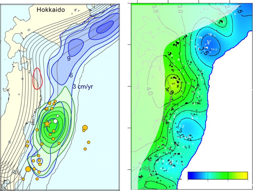
Uchida Progress in Earth and Planetary Science              (2019) 6:40                                                                  Page 2 of 21

Nadeau and McEvilly 1999; Igarashi et al. 2003) and esti-                    discuss how they compare with estimates from geodetic
mating various properties of slow slip including postseis-                   data.
mic slip (e.g., Uchida et al. 2004; Hayward and Bostock
2017), spontaneous slow slip episodes (e.g., Nadeau and                      Review
McEvilly 2004; Uchida et al. 2016b) and preseismic slip                      Model of repeating earthquakes and their relation with
(e.g., Kato et al. 2012). These observations of slow slip                    slow slip
suggest they are essential fault deformation process to-                     Repeating earthquakes are interpreted as representing
gether with regular earthquakes. Therefore, it has be-                       repeated ruptures of a fault patch that are driven to fail-
come increasingly important to clarify the optimal                           ure by loading from aseismic creep on the surrounding
method of selecting repeating earthquakes and obtaining                      fault surface. Therefore, the seismic slip of repeating
reliable measurements of slow slip from repeating                            earthquakes can be related to the fault creep in the sur-
earthquakes.                                                                 rounding area during the interseismic period. Figure 1
  In this article, I first review the general procedure for                  shows the general concept of how repeating earthquake
detecting repeating earthquakes. Then, I discuss appro-                      analysis can be used to estimate fault creep. The cumu-
priate parameters for selecting repeating earthquakes                        lative slip of repeating earthquakes can be assumed to be
based on waveform similarity which suggest the import-                       equal to the creep on the surrounding fault area of the
ance of selecting an appropriate frequency range. I also                     repeater patch. Observations of repeating earthquakes
discuss the triggered sequences and their characteristics                    provide a useful estimate of slow slip based on their ac-
in event intervals. Next, I review the procedure for                         tivity pattern.
quantifying the slow slip associated with repeating se-
quences, including the scaling relationship between                          Detection method
earthquake magnitude and slip. Lastly, I will provide an                     An important condition for repeating earthquakes that
overview of the application of repeating earthquakes for                     can be used to estimate the amount of slow fault slip is
estimating slow fault slip in various tectonic settings and                  whether the earthquakes represent repetitive rupture on

                                                      Similar
                                                      waveforms
                                                                                      creeping area
                                                                               Slip
                                                   Tren
                                                        c

                                                                                                   Time
                                                      h

                                              ep
                                           cre
                                ep
                             cre
                                                                                      seismic patch
                                                                               Slip

                                                                te
                                                             Pla
                                        ep
                                     cre

                                                   repeating
                                                   earthquakes                                    Time

 Fig. 1 Schematic model of the environment where repeating earthquakes occur in a subduction zone. The repeating earthquakes occur on a
 seismic patch (black spots) in the creeping area of the plate boundary. They produce similar waveforms when observed by the same station (left
 top) because the seismic patch is loaded by creep in the surrounding area and repeat rupture at the same place. The creeping area (slip shown
 in red in the right top panel) and repeating earthquake patch (slip shown in red in the right bottom panel) undergo almost the same long-term
 cumulative slip because they are located on neighboring plate boundaries. The dashed line shows slip at neighboring area (seismic patch for
 creeping area and vice versa). Please note the patch for the repeating earthquake may have slip in the interseismic period (Beeler et al. 2001) but
 the relationship between the slip at the creeping area and the slip at patch for repeating earthquakes holds in that case too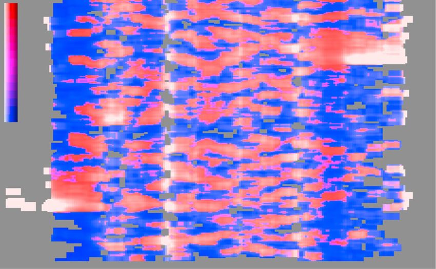
Uchida Progress in Earth and Planetary Science                        (2019) 6:40                                                           Page 3 of 21

a common patch (being co-located) or not. An example                                         (Ellsworth 1995; Waldhauser and Schaff 2008; Yu 2013).
of co-located earthquakes (repeaters) and their wave-                                        Repeating earthquakes have similar waveforms, and thus
forms are shown in Fig. 2. Their location estimates show                                     their time differentials can be obtained accurately from
overlapping source areas (Fig. 2a) and their waveforms                                       waveform cross-spectra or waveform cross-correlations
are very similar (Fig. 2c). Both source areas and wave-                                      (Waldhauser and Ellsworth 2000) (Table 1).
form characteristics can be used to detect repeating                                           The double-difference method (Waldhauser and Ells-
earthquakes, as detailed below.                                                              worth 2000) is one popular method of obtaining precise
                                                                                             locations with an uncertainty of as little as a few meters
Detection of small repeating earthquakes from                                                (Waldhauser et al. 2004). Other methods used to esti-
hypocenter locations                                                                         mate relative locations include a master-event algorithm
Determining hypocenters is a straightforward way to con-                                     which is used by Yu (2013). Conditions for obtaining
firm overlapping source areas and to detect repeating                                        precise locations include good clocks (timing accuracy)
earthquakes. The precision of relative hypocenter loca-                                      and a sufficient number of data (stations) with good
tions, however, should be high enough compared with the                                      spatial distribution. Chen et al. (2008) used a
earthquake source sizes to confirm the co-location. Most                                     double-difference method based on S-P time for estimat-
previous works have utilized waveform-based differential                                     ing location when working on the data with clock
time to obtain precise relative earthquake locations                                         uncertainties.

                140˚                    141˚   142 ˚E
  (a)                                                         East                         (c)   FUT UD   41.4˚N 141.8˚E 66km                 1-15Hz
          N                        -500
                                     -500
                                                              0                           500m
         42˚
                                  500
                                                                                                 1994 0730 1301 M=3.4

         41˚                                                                                     1996 06041459    M=3.5

                              50 km

                                                                                                 19971019 0237    M=3.3
        North

                                  0

                                                                                                 1999 0419 0708 M=3.2

                                                                                                 2000 1012 0549 M=3.2

                                                                         100m

           500m                                                                                  2002 11161244 M=3.5

  (b)
                                                                                                 2004 0314 0019 M=3.4
                Cumulative slip

                                                  20
                                                  0 (cm/yr)
                                                                                                 20051016 0152 M=3.4
                                                                                    100
                                                                                    cm
                                                                                                    P                           S
                                   1992 1994 1996 1998            2000 2002 2004 2006               0        10           20          30      40

                                                         Time (year)                                                  Time (second)
 Fig. 2 An example of a repeating earthquake source locations, b cumulative slip, and c waveforms for one sequence 65 km deep in the
 northeastern Japan subduction zone (see inset in a for the location) (after Uchida et al. (2006)). The centroid locations are based on double-
 difference hypocenter estimation using the cross-spectrum method to find the precise differential time. Source sizes are estimated using a 75
 MPa stress drop. The cumulative slip in b was calculated by using the seismic moment-slip relationship by (Nadeau and Johnson 1998). The
 waveforms in c are the vertical component observed at station FUT (Δ = 190 km) in Honshu, Japan, filtered in the 1–15 Hz range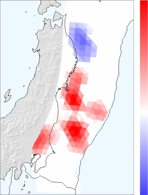
Uchida Progress in Earth and Planetary Science              (2019) 6:40                                                                         Page 4 of 21

Table 1 Comparison of repeating earthquake selection and slip estimation methods for selected papers
References         Region          Detection method          Time window              Frequency        M range              Slip         Comments
                                                                                      range                                 scaling
Nadeau and      Parkfield,         CC ≧ 0.98                 –                        –                N/A (M − 1 to 5      N&J
McEvilly (1999) California                                                                             used)
Igarashi et al.    Tohoku,         CC ≧ 0.95                 40 s                     1–4 hz           4.6 ≧ M > =3         N&J
(2003); Uchida     Japan                                                                               (Igarashi et al.),
et al. (2003)                                                                                          M ≧ 2 (Uchida et
                                                                                                       al.)
Nadeau and      San Andreas        CC, Coh, visual         –                          –                3.4 ≧ M ≧ -0.4       N&J
McEvilly (2004) fault              inspection, relocation,                                                                  (constants
                                   arrival time analysis                                                                    different)
Matsubara et       Hokkaido,       CC ≧ 0.95                 40 s or until 5 s        1–8 Hz           M≧2                  N&J
al. (2005)         Japan                                     after S arrival
Kimura et al.      Kanto, Japan    CC ≧ 0.95                 2 s before P arrival     1–20 Hz          4.56 ≧ M ≧ 2.0       N&J
(2006)                                                       to 5 s after S arrival
Uchida et al.      Miyagi-oki,     Coh ≧ 0.95                40 s                     1–8 Hz           4.8 ≧ M ≧ 2.5        N&J          Upper range of M is
(2006, 2009a,      Tohoku                                                                                                                from Uchida et al.
b, 2011)           Japan                                                                                                                 (2009a, 2009b)
Rau et al.         Longitudinal    waveform (CC) and         10.5 s (CC), 2.5 s       2–18 Hz          4.6 ≧ M ≧ 2.1        N&J          CC has several
(2007)             valley fault,   differential S-P time     (differential S-P)                                                          thresholds
                   Taiwan
Chen et al.        Chihshang       CC and differential S-    10.5 s (CC), 2.5 s       2–18 Hz          3.7 ≧ M ≧ 1.9        N&J          CC has several
(2008)             fault, Taiwan   P time                    (differential S-P)                                                          thresholds
Lengliné and       Parkfield,      Coh≧0.9 and location 1.28 s (P wave)               1.5–18 Hz        M ≧ 1.2              N&J          3 MPa stress drop,
Marsan (2009)      California      (overlapping > 70%)                                                                                   magnitude
                                                                                                                                         difference < 0.2
Igarashi (2010)    Japan           CC ≧ 0.95                 P arrival to 3 s after   1–4, 2–8, and    M≧2                  N&J          Frequency range
                                                             S arrival                4–16 Hz                                            depends on
                                                                                                                                         magnitude.
Li et al. (2011)   Longmen         CC ≧ 0.9 and internal 1 s before a P arrival 1–10 Hz                2.8 ≧ M ≧ 0.9        Crack        Average recurrence
                   Shan fault,     consistency of time   to 5 s after S arrival                                                          interval of > 100
                   China           picking                                                                                               days
Yamashita et       Hyuganada,      CC ≧ 0.95                 40 s                     2–8 Hz           4.3 ≧ M ≧2.5         N&J          Duration < 3 years
al. (2012)         southwest                                                                                                             removed, focal
                   Japan                                                                                                                 mechanism checked
Kato et al.        Tohoku,         Matched filter            P-wave onset to 4 s      1–4, 2–8, and                         N&J          Frequency range
(2012)             Japan           detection and             after direct S-wave      4–16 Hz                                            depends on
                                   CC ≧ 0.95                 arrival.                                                                    magnitude
Uchida et al.    Tohoku,           Coh ≧ 0.95 (1–8 Hz)       40 s                     1–8 Hz or        M ≧ 2.5              N&J
(2013, 2016a, b) Japan             or Coh ≧ 0.8 (1/2–2                                around the
                                   fc)                                                corner
                                                                                      frequency (fc)
Yu et al. (2013) Tonga–            CCC ≧ 0.8                 30 s                     0.8–2.0 Hz       5.7 ≧ M ≧ 4.7        N&J
                 Kermadec–
                 Vanuatu
Taira et al.       San Juan      CC and Coh ≧0 .95           51.2 s (M ≧ 2), 5.12 s 1–8 Hz (M ≧ 2),    3.5 ≧ M ≧ 0.5        N&J
(2014)             Bautista, San                             (M ≦ 2.5)              8–24 Hz
                   Andreas fault                                                    (M ≦ 2.5)
Meng et al.        Northern        CC≧0.95                   3 s before a P arrival 1–8 Hz (3 >        4.8 ≧ Mw ≧ 2.9       N&J
(2015)             Chile                                     to 10 s after S arrival Mw ≧ 2.5)
                                                                                     1–4 Hz
                                                                                     (Mw ≧ 3)
Mavrommatis        Tohoku,         Co ≧ 0.95 (1–8 Hz) or 40 s                         1–8 Hz or        M ≧ 2.5              Beeler       Event selected by
et al. (2015)      Japan           Coh ≧ 0.8 (1/2–2 fc)                               around the                                         M, variation in M
                                                                                      corner                                             and duration
                                                                                      frequency (fc)
Gardonio et al. Kanto, Japan       Coh ≧ 0.90 and            5.12 s                   1.5–8 Hz         M ≧ 1.0              No slip      Magnitude
(2015)                             location (overlapping                                                                    estimate     difference < 0.5
                                   > 50%)
Uchida Progress in Earth and Planetary Science (2019) 6:40 Page 5 of 21
Table 1 Comparison of repeating earthquake selection and slip estimation methods for selected papers (Continued)
References Region Detection method Time window Frequency M range Slip Comments
range scaling
Dominguez et Middle CC and 25.6 s 1–8 Hz 4.5 ≧ M ≧ 2.5 (A), N&J
al. (2016) America Coh ≧ 0.90(threshold 4.5 ≧ M ≧ 3.1 (B)
Trench, A), CC, and
Mexico Coh ≧ 0.95(B)
Schmittbuhl et Marmara CC ≧ 0.9 15 s 1–10 Hz 2.5 > M > 1 Crack
al. (2016) fault, Turkey
Yao et al. Nicoya Matched filter 6s – 3.2 ≧ M ≧ 0.5 Crack Template events
(2017) Peninsula, method (mean have S/N ≧ 5 for
Costa Rica CC ≧ 0.9) more than 9 traces
Materna et al. Mendocino Coh ≧ 0.97 30 s before the P 0.5–15 Hz (S/ 3 ≧ M ≧ 1.5 N&J
2018) Triple arrival to 20 s after N ≧ 5)
Junction the P wave arrival
CC waveform cross-correlation, Coh waveform coherence, N&J Nadeau and Johnson (1998)‘s scaling relationship (Eq. (1)), Beeler: Beeler et al. (2001)’s relationship
(Eq. (2)), Crack crack model (Eq. (3) or others)
After obtaining repeaters’ relative locations, the source exactly the same waveforms if the medium and record-
size is used to evaluate how they overlap. The source ing system has not changed. The similar waveforms at a
size of repeaters can be estimated from the corner fre- particular station indicate small inter-event distances
quency of their waveforms (e.g., Uchida et al. 2012; Ima- and similar focal mechanisms (Menke 1999; Nakahara
nishi et al. 2004) or using waveform inversion (e.g., 2004). This is a less exact way to confirm co-location
Okada et al. 2003; Dreger et al. 2007; Kim et al. 2016). but represents a powerful and relatively robust proced-
These studies use spectrum ratios or empirical Green’s ure if we choose the analysis parameters carefully. The
functions to take into account attenuation and other waveform-similarity based detection is popular than the
path effects. However, these techniques are generally detection from hypocenter locations (see “Detection
complicated and too time-consuming, if we want to method” section column in Table 1) most probably due
utilize them for many possible repeater candidates. A to their relatively smaller requirements for the amount
popular method for obtaining source size is to assume a and quality of data (e.g., the number of stations, station
stress drop based on regional studies and use the rela- distribution, and timing accuracy of station clocks). This
tionship between seismic moment (M0) and source ra- method needs only one station that is available through-
dius (r) (Eshelby 1957), out the analysis period, although using multiple stations
provides a more robust detection.
r ¼ ðð7=16ÞðM 0 =Δσ ÞÞ1=3 : ð1Þ
Figure 2a shows an example of double-difference relo- Quantification of waveform similarity between earthquakes
cations in which a stress drop of 75 MPa was used for Two major methods for evaluating the waveform simi-
the source size. The seismic moment used here was esti- larity are cross-correlation analysis and cross-spectral
mated by the formulas of Hanks and Kanamori (1979): analysis of waveform coherence (Poupinet et al. 1984)
(Table 1). The waveform cross-correlation coefficient is
logðM 0 Þ ¼ 1:5M þ 9:1 ð2Þ P
defined as CðτÞ ¼ N1 N t¼1 f x ðtÞ f y ðt þ τÞ, where fx and fy
Note that the assuming low stress drops results in a are two time series (e.g., waveforms) of earthquakes x
large slip radius and apparent overlapping may occur for and y with N discrete samples and τ is the lag time. We
more distant events. The stress drops used in several can obtain the maximum cross correlation coefficient
studies are listed in Table 1. The minimum source over- (CC) by varying the lag time. Waveform coherence is de-
rffiffiffiffiffiffiffiffiffiffiffiffiffiffiffiffiffiffi
lap used as a condition for repeating earthquakes in pre- jS xy ðωÞj2
fined as cohðωÞ ¼ S xx ðωÞS yy ðωÞ . Here, Sxy(ω) is the cross
vious studies range from 50 to 70% in the previous
studies (Lengliné and Marsan 2009; Waldhauser and spectrum between earthquakes x and y that is calculated
Ellsworth 2002; Gardonio et al. 2015). from the Fourier transform of the original waveforms (fx
and fy). We usually use the average of coherence (Coh)
Detection of small repeating earthquakes from waveform for a certain frequency range. The cross-correlation and
similarities cross-spectrum methods are very similar, other than that
We can select repeating earthquakes by taking advantage the frequency range is set before the calculations for
of the idea that earthquakes that ruptured the same evaluating similarity are done in cross-correlation while
source area with the same rupture process should have selection is done after the calculations in theUchida Progress in Earth and Planetary Science (2019) 6:40 Page 6 of 21
cross-spectrum method (Schaff et al. 2004). The Parameters for better selection of repeating earthquakes
co-location of overlapping sources is judged from the from waveform similarities
values of CC or Coh for a pair of waveforms recorded at Waveform similarity provides less direct evidence for
the same station having the same or equivalent record- overlapping sources than hypocenter colocation and it
ing system throughout the study period (Fig. 1). Note requires careful analysis to obtain a reliable repeater
that changes in the recording system and/or the charac- catalog. In this section, I discuss finding better selection
teristics of the seismometers used may result in apparent parameters including an optimal choice of time windows
changes in waveforms if the responses are not corrected. and lower and upper limits of analysis frequency.
The maximum values of CC and Coh are 1 and a large
CC or Coh value (usually 0.95 or higher are chosen) sug- Analysis time window
gests nearly identical waveforms. In calculating waveform similarity, the length of the
To reduce computation time, evaluations of CC or sample time window is an important factor that affects
Coh are usually done for event pairs within a certain the value of CC or Coh. Time windows are usually set to
inter-event distance based on the routine hypocenter contain both P and S phases to assure the same P-S time
locations of the events. The summation of hypocenter and thus the same hypocentral distance (e.g., Uchida et
location uncertainties for the pair is a good basis for al. 2003; Igarashi et al. 2003). A longer time window re-
determining a search volume because co-located duces the possibility of high cross-correlation or coher-
events may be mislocated at points that are separated ence by chance but may contain low signal-to-noise
by their uncertainties. Search radii in previous studies ratio coda waves. Some studies use a variable window
have been 80 km in the Tonga–Kermadec–Vanuatu length, depending on the S-wave arrival time (e.g.,
subduction zones (Yu 2013), 30 km in the Tohoku Kimura et al. 2006; Taira et al. 2014; Meng et al. 2015),
and Mendocino triple junctions (Igarashi et al. 2003; but the others use a fixed value that is long enough for
Materna et al. 2018), but smaller values may be ap- the target earthquakes (e.g., Matsubara et al. 2005;
propriate in more densely instrumented areas. Most Uchida et al. 2003; Igarashi et al. 2003) (Table 1). The
studies calculate CC or Coh for individual stations signal-to-noise ratio (S/N ratio) is also considered in
that are averaged later (Table 1). The matched filter some cases (Materna et al. 2018).
method (Gibbons and Ringdal 2006; Shelly et al.
2007), which scans continuous waveforms and utilizes Lower limit of analysis frequency range
both waveform similarity and consistency of travel Selection of proper frequency range is important not
times between stations has also been used to detect only to reduce the effect of noise but also to make the
repeaters (Yao et al. 2017). CC/Coh value more informative for judging whether the
sources overlap or not. In general, waveforms at too low
frequencies do not have enough resolution to distinguish
Formation of repeater sequence from pairs of repeaters between nearby non-overlapping and overlapping
Once repeating earthquake pairs are defined from hypo- events.
center locations and/or waveform similarities, a repeat- One method for finding a suitable lower limit of the
ing earthquake sequence can be formed from the pairs. frequency range is to consider the “quarter wavelength
A simple equivalence class algorithm (Press et al. 2007) rule” (Geller and Mueller 1980) for waveform similarity.
is used in many studies (Igarashi et al. 2003; Uchida et Similar seismograms at a given frequency suggest that
al. 2003; Peng and Ben-Zion 2005; Materna et al. 2018; their first-Fresnel zones (the prolate ellipsoidal space be-
Meng et al. 2015; Yao et al. 2017; Kimura et al. 2006; tween two points) overlap (Geller and Mueller 1980;
Nadeau et al. 1995). The algorithm groups pairs that Ellsworth 1995). In other words, two events located
share the same events into the same repeater sequence. within a quarter wavelength cannot be separated based
In other words, if event pairs (A, B) and (B, C) are re- on waveform similarity even if they do not overlap (Gel-
peater pairs, events A, B, and C are grouped into one ler and Mueller 1980). Thus, the use of high-frequency
sequence regardless of the similarity/overlapping be- waveform data whose quarter wavelengths are smaller
tween A and C. Another method employed to com- than their rupture dimension is necessary to reduce the
bine pairs is a clustering algorithm based on the possibility of non-overlapping events. Taking this into
unweighted pair group method with arithmetic mean account, when the frequency (f ) condition that has over-
(Romesburg 2004; Hayward and Bostock 2017). This lapping events with the same source size can be distin-
grouping produces sequences in which the average guishable is f ≥ vs/4r, where vs is shear wave speed and r
CC/Coh of each member event of a sequence with all is the source radius. Since the source size usually de-
other members in the sequence is greater than the pends on the earthquake size (magnitude, seismic mo-
desired CC/Coh threshold. ment), the optimal lower limit of the frequency rangeUchida Progress in Earth and Planetary Science (2019) 6:40 Page 7 of 21
also depends on earthquake size. The recommended are selected for the analysis. The corner frequencies are
minimum frequency to be included in the repeater ana- calculated from the following formula by Sato and Hira-
lysis is shown by the gray line in Fig. 3a. Here, the sawa (1973)
source sizes (radii r) of the events are calculated from
magnitudes (M) assuming the circular crack model and f 0 ¼ Cν=2πr; ð3Þ
stress drops (Δσ) of 10 MPa, using Eq. (2) by Hanks and
Kanamori (1979) and Eq. (1) by Eshelby (1957). and Eq. (1), where ν is the phase velocity (4.4 km/s) and
The effect of the choice of the lower limit for the ana- C is a constant. We assumed C to be 1.9 and the stress
lysis frequency range can be examined from inter-event drop to be 10 MPa. Please note that the frequency range
coherences whose source location and sizes are precisely (1–2 Hz) is below the frequency range appropriate for
estimated. The off-Kamaishi earthquake is one such ex- selecting repeaters for most of the analyzed events of
ample (Fig. 4a) and Fig. 5 demonstrates how coherence magnitudes 2.4–3.6 (Fig. 3a).
changes with inter-event distance for pairs of earth- The relationship between inter-event distance and co-
quakes in the earthquake cluster that contain repeater herence shows that coherence decreases significantly if
sequences. Here, the distances are normalized by the the pairs do not overlap (normalized distance > 1) for
fault radius (inter-event distances are divided by the sum analysis of the frequency range near the corner fre-
of the fault radii of the two earthquakes). The centroids quency (Fig. 5a). It also shows that the radius ratio (the
and source sizes used to calculate the normalized dis- source radius of the smaller event divided by that of the
tance are respectively constrained by the larger event) also affects the value of coherence. The co-
double-difference method using waveform cross-spectra herence threshold (0.8) used in (Uchida and Matsuzawa
and spectral ratio analysis and have uncertainties of less 2013) corresponds to a minimum radius ratio of about
than ~ 30 m and ~ 6%, respectively (Uchida et al. 2012). 0.6. On the other hand, for the low-frequency range (1–
For the coherence calculations, the time window is 40 s 2 Hz, Fig. 5b), coherence does not drop significantly for
and two frequency ranges extend with half to twice the non-overlapping events (normalized distance > 1) and
corner frequency for the smaller event of each pair the coherence at each station (small white circles) is
(Fig. 5a) and a fixed frequency range of 1–2 Hz (Fig. 5b) sometimes large (> 0.95) for non-overlapping events.
(a) (b)
100 High frequency range : 100 Chen Kimura Yamashita
Fr waveform may dissimilar 2008 2005 2012
eq due to rupture
ue Rau 2007
nc
Frequency (Hz)
Frequency (Hz)
complexiety Taira
y
ra
co 2014
rn Matsubara 2005
10 ng
er 10
e Lengline Uchida 2009
ap fre
ra
pr qu 2009 Dominguez
op
di
Gardonio 2016
en
us
re
at cy 2015 Igarashi 2010
=
e Kato 2012
1 fo 1 Materna
vs
r
/4
re 2018
f
pe Uchida 2013
at co
er Schmittbuhl Li Igarashi Meng rn
se 2016 2011 2003 2015 er
Low frequency range: le fre
ra
0.1 ct 0.1 qu
di
waveform similarity io Yu en
us
n cy
=
cannot discriminate 2013
vs
/4
neighbouring events
f
0.01 0.01
0 2 4 6 8 0 2 4 6 8
Magnitude Magnitude
Fig. 3 a Frequency and magnitude ranges suitable for repeater detection from waveform similarity based on considerations of source size and b
ranges used in previous studies. Black and gray lines respectively show the corner frequency and the condition where the resolution is equal to
the fault radius for a 10 MPa stress drop. Dashed black and gray lines are the same but for a 1 MPa stress drop. Frequencies larger than the corner
frequency (blue area) are considered to be inappropriate because the rupture process, including the initiation point and propagation may affect
waveforms’ shape. Having the resolution lower than the fault radius (radius ≤ vs/4f) (red area) is also inappropriate because non-overlapping
events can also have similar waveforms. In b, frequency and magnitude ranges are plotted for the studies listed in Table 1. Note that only the
first author and publication year are shown for each study and some studies used not only waveform similarity but also hypocenter location or
other conditions to confirm repeaters. When the maximum size of detected earthquakes is not reported, the upper bounds of magnitude are
not shownUchida Progress in Earth and Planetary Science (2019) 6:40 Page 8 of 21
(a) 1000 (b)
fc: observed
1.0
500 2001 0.8
A
Coherence
North (m)
C
B
0.6
0
0.4
-500
2008 0.2 2001-2008
event
-1000
0.0
-1000 -500 0 500 1000 1 10
Distance along dip (m) Frequency (Hz)
Fig. 4 a Slip area distribution in the off-Kamaishi earthquake cluster. Circle size denotes rupture dimension estimated from corner frequencies.
Small bars show centroid location uncertainties. The labels 2001 and 2008 indicate M~ 4.8 repeating earthquakes in those years. The earthquakes
labeled A–C are events with magnitudes 2.4–3.6 that occurred from 1995 to 2008. This figure is modified from Uchida et al. (2012). b Coherence
dependence on frequency for the waveforms of the 2001 and 2008 M~ 4.8 repeating earthquakes for 11 stations. A time window of 40 s was
used for the calculation. The vertical line shows the observed corner frequency from spectral ratio analysis (Uchida et al. 2012)
d Radius Ratio (b/a)
a b
0.00 0.25 0.50 0.75 1.00
(a) (b)
1.0 1.0
0.8 0.8
Coherence
0.6 0.6
0.4 0.4
0.2 0.2
Frequency: Frequency:
1/2 fc - 2 fc 1-2 Hz
0.0 0.0
0 1 2 3 4 5 0 1 2 3 4 5
Normalized Distance (d/(a+b)) Normalized Distance (d/(a+b))
Fig. 5 Relationship between normalized distance (distance between the centroids of a pair of earthquakes divided by the summation of the
source radii) and coherence for the off-Kamaishi earthquake cluster in northeastern Japan (Fig. 4a). a, b The results from the frequency range
around the corner frequency of the smaller earthquake (1/2 fc–2 fc) (Uchida and Matsuzawa 2013) and 1–2 Hz, respectively. Normalized distances
0, 1, and > 1 indicate identical centroids, contacting sources, and sources with no overlap as shown in top left insets. Black dots show values at
each station and colored dots are values averaged for each pair of earthquakes. The color represents the radius ratio (the radius of the smaller
earthquake divided by the radius of the larger earthquake). The centroid locations and source sizes used for the calculations are from Uchida et
al. (2012) where the centroids are estimated by the waveform-based double-difference method and the source sizes are estimated from corner
frequencies using stacked spectrum ratios. Uncertainties in the normalized distance and radius ratio are less than 0.2 and 0.12, respectivelyUchida Progress in Earth and Planetary Science (2019) 6:40 Page 9 of 21
This suggests the possibility of selecting Evaluation of the repeater catalog and optimization of
non-overlapping events in this frequency range even if a the repeater selection procedure
large coherence threshold is employed. In summary, an Once repeaters are selected by any method, it is also im-
appropriate lower limit of the frequency range, which is portant to evaluate the catalog and use it to optimize the
dependent on the source size is important in selecting repeater selection method. Since the present aim of
repeaters using waveform similarity. selecting repeating earthquakes is to track the slip his-
tory at a particular point, it is both important to elimin-
Upper limit of analysis frequency range ate triggered sequences that are not overlapping events
The upper limit of the appropriate frequency range is con- and avoid missing events.
sidered to be related to the variability of the rupture process.
The waveforms at high frequencies depend on rupture Triggered sequence in the repeater candidates
process variations within the slip area that can be different Neighboring events are often triggered by each other
for repeating earthquakes even when sharing the same (Rubin et al. 1999; Chen et al. 2013). Rubin et al. (1999)
source area. In other words, the rupture initiation point (hy- studied the microseismicity in the creeping section of
pocenter) within a patch, slip directivity, etc. may change the San Andreas Fault zone based on precise hypocenter
from event to event reflecting heterogeneous stress and locations. They showed that the second events of con-
strength within the patch (Kim et al. 2016; Shimamura et al. secutive event pairs occurred outside the slip area of the
2011; Bouchon 1997; Murray and Langbein 2006; Vidale et first event assuming a 10 MPa stress drop. This suggests a
al. 1994) but this difference in dynamic process does not stress shadow at the slip area of the first event and trigger-
affect the total slip amount within the slip area. Figure 4b ing of the second event outside of the slip area of the first
shows the frequency dependence of coherence between the event (Fig. 6). However, it is sometimes difficult to distin-
waveforms of the 2001 and 2008 M~ 4.8 off-Kamaishi re- guish neighboring events from co-located (repeating)
peating sequence (Fig. 4a). Although these sequences have events because they have both high waveform similarity
almost completely overlapping source areas (Fig. 4a), the and similar locations. For example, Bouchon et al. (2013)
Coh at frequencies larger than the corner frequency signifi- proposed repeated foreshock occurrences for the 1999
cantly decrease from 1. Such a decrease in coherence in fre- Izmit earthquake from the events’ waveform similarity,
quency ranges higher than the corner frequency has also but Ellsworth and Bulut (2018) suggested a triggered cas-
been reported for other repeating sequences (Hatakeyama et cade of rupture for neighboring areas based on their esti-
al. 2016). This means the use of frequency ranges lower than mate of precise location and slip areas.
the corner frequency reduces the possibility of excluding In addition to location or waveform difference, tem-
events with different rupture patterns but co-located (re- poral characteristics of triggered sequences can also be
peating) events. The corner frequency dependence on earth- used to distinguish repeating earthquakes from the trig-
quake magnitude (assuming the circular crack model) is gered sequence. Lengliné and Marsan (2009) clarified
shown in Fig. 3a. Here, I assumed 1 and 10 MPa stress drops features of triggered sequences from repeater candidates
and used Eqs. 1, 2, and 3. This line can be used as the rough selected based on waveform similarity and event over-
standards of the upper limit of analysis frequency range. lapping ratios in Parkfield, CA (Fig. 7). They looked at
Most studies apply band-pass filtering before calculat- the frequency distribution of recurrence intervals. The
ing cross-correlation or selecting a frequency range in frequency distribution of events interval follows a power
evaluating coherence (Table 1) with a single frequency law decay with increasing event interval for events with
range. The frequency and magnitude ranges of detected intervals shorter than 10% of the sequence average. The
repeating earthquakes are shown in Fig. 3b. Since the decay rate of earthquake frequency with increasing inter-
optimal frequency range for repeater selection from val is consistent with Omori’s law and indicative of a
waveform similarity depends on the source size as dis- triggering process. The spatial distribution of
cussed in this and previous sections, the use of a fre- probably-triggered-events (events with interval times
quency range that depends on earthquake size 10% or less of the average recurrence interval) is not
(magnitude) will be better for selecting repeating earth- spatially concentrated (i.e., the events are not co-located)
quakes over a wide magnitude range. Igarashi (2010), (Fig. 7b) whereas events with interval times longer than
Meng et al. (2015), and Taira et al. (2014) used multiple 10% of the average show tightly concentrated event loca-
frequency ranges depending on earthquake magnitude tions (Fig. 7c). This is consistent with the concept that it
(Fig. 3b). Uchida and Matsuzawa (2013) used frequency is difficult to reload a fault patch in a very small time
ranges relative to magnitude dependent corner frequen- interval, except for special conditions such as fast load-
cies (Fig. 3b). These studies succeeded in detecting re- ing caused by postseismic deformation from large earth-
peaters over a relatively wide magnitude range (Table 1, quakes, and we need careful evaluation for very short
Fig. 3b). interval repeater candidates.Uchida Progress in Earth and Planetary Science (2019) 6:40 Page 10 of 21
Optimization of repeater selection
As described in the previous section, an extremely short
event interval can be a useful diagnostic feature for iden-
tifying triggered sequences among the sequences se-
lected from waveform similarity and hypocenter
locations, which have inevitable uncertainty in the detec-
tion (Lengliné and Marsan 2009; Materna et al. 2018; Li
et al. 2011). We want to exclude triggered events that
occur adjacent to each other and that often occurs over
a short time interval. When setting the threshold for re-
peaters, the fraction of earthquakes with very short in-
tervals (minutes to days) becomes unacceptably large if
the selection criterion being used is too loose. Figure 8
shows an example of the frequency distributions of re-
peater candidates’ recurrence intervals using two differ-
ent coherence thresholds (0.8 and 0.95) for off-Tohoku
earthquakes (Uchida and Matsuzawa 2013). The other
detection conditions (calculation of coherence for a fre-
quency range of 1–8 Hz and a time window of 40 s) are
the same. The figure shows that when an inadequately
low coherence threshold of 0.8 is used, the fraction of
very short earthquake intervals becomes large. The fre-
quency of earthquake interval increases with decreasing
time interval in the year scale (Fig. 8a), day scale
Fig. 6 Relationship between the magnitude of the first event and (Fig. 8b), and minutes scale (not shown), suggesting that
distance to the second earthquake for consecutive earthquakes in aftershock (triggered) sequences dominate for
the creeping section of the San Andreas fault (after Rubin et al. short-interval and relatively less-similar pairs. For the
1999). Diamonds indicate that the vertical separation between the larger (preferred) coherence threshold (0.95), the fre-
events exceeds the horizontal separation; crosses indicate the
quency peaks at ~ 1 year and the frequency decreases
reverse. The diagonal line is the estimate of earthquake radius
derived from the moment-magnitude relation of Abercrombie when the interval is short, which probably reflects not
(1996), assuming a stress drop of 10 MPa enough time to load the same fault patch. The drastic
change in the numbers of short-interval events brought
about by increasing the coherence threshold suggests
that most of the short-interval events have relatively low
coherence and can be interpreted as triggered events
(a) (b) (c)
Along depth distance
Probability density
Normarized density
Fig.b Fig.c
Recurrence interval Along fault distance
Fig. 7 Behavior of repeater candidates dependent on recurrence intervals. a Probability density for normalized recurrence intervals. The
normalized recurrence intervals are defined by the interval divided by the averaged recurrence interval for sequences with four or more
earthquakes. The dashed line shows a power law decay. b, c Spatial distribution for b short-term (normalized recurrence intervals < 0.1) and c
long-term (normalized recurrence intervals > 0.1) earthquakes in a repeating sequence compared to the centroid of the sequence. After Lengliné
and Marsan (2009)Uchida Progress in Earth and Planetary Science (2019) 6:40 Page 11 of 21
(a) (b)
700 300
600 threshold = 0.8
500 threshold = 0.95 200
Number
Number
400
300
100
200
100
0 0
0 5 10 0 10 20 30
Time (year) Time (day)
Fig. 8 Frequency distribution of the intervals of successive events using coherence thresholds of 0.8 (gray) and 0.95 (black). a 0 to 10-year range
in 0.25 year bins. b 0 to 31 days in 1-day bins. The frequency range is 1–8 Hz and data used was from 1984 to 2006 offshore Tohoku
that are close but not co-located, although occasionally Nadeau and Johnson (1998) proposed the following
lower-coherence repeaters may occur after large earth- empirical relationship between fault creep (d; cm)
quakes due to their slip dependency on pore pressure and repeater seismic moment (Mo; dyne·cm) which
(Lengliné et al. 2014), fault healing (McLaskey et al. is also shown in Fig. 9.
2012), and loading rate (Hatakeyama et al. 2017).
The dependence of repeater catalogue on selection d ¼ 10−2:36 M o0:17 : ð4Þ
method is extensively examined in Lengliné and Marsan
(2009) and Materna et al. (2018). The inclusion or exclusion
They used observed data of the moment release rate
of short-recurrence (probably triggered) sequences has a
of repeaters and an average regional geodetic creep rates
very large impact on which events are selected as repeaters,
in Parkfield and Stone Canyon to build the empirical re-
and inter-event timing is one of the most important features.
lationship. The Parkfield repeaters are selected by wave-
For the estimation of slow slip from repeaters, the strict
form cross-correlation and visual inspection (Nadeau et
threshold can eliminate triggered sequence but may result
al. 1995; Zechar and Nadeau 2012) and the Stone Can-
in misdetection due to their uncertainty in location or wave-
yon repeaters are selected by hypocenter locations (Ells-
form similarity decrease by noise. To this end, the
worth and Dietz 1990). This relationship has been used
inter-event time can be used to find appropriate repeater se-
to estimate creep from repeating earthquakes in various
lection parameters. Another method to utilize inter-event
areas (Table 1) (Chen et al. 2007; Uchida et al. 2003;
time is to simply discard events with short inter-event times
Igarashi et al. 2003). Variations in the empirical relation-
from repeater candidates to obtain continuous repeating
ship have been posited as d ¼ 10−1:090:2 M o0:1020:3
earthquakes that are more likely reflect long-term fault slow
(Nadeau and McEvilly 2004) who re-estimated the em-
slip. As an example of inter-event time filtering, Igarashi et
pirical scaling constants for larger sections along the San
al. (2003) used a 3-year duration threshold for selecting
burst-type and continuous type events and Li et al. (2011) Andreas fault, and d ¼ 10−1:530:37 Mo0:100:02 (Khoshma-
used a sequence averaged recurrence interval of 100 days to nesh et al. 2015) who re-estimated constants in the
filter out triggered sequences occurring on closely spaced model from high-resolution spatiotemporal modeling of
but not overlapping fault patches. the slip on the San Andreas fault.
The scaling by Nadeau and Johnson (1998) sug-
Estimation of slow fault slip from repeating earthquakes gests that T r ∝M 1=6
o , where T r represents the recur-
Based on identified repeaters, we can estimate the rence interval. This relationship is different from the
cumulative slip of repeating earthquakes that tells us generally accepted relationship T r ∝M 1=3 o which is de-
about the slow slip history in the area surrounding rived from the standard assumption of constant
the repeater patch. There are three types of models stress drop (Nadeau and Johnson 1998) and dis-
that can be used to estimate slip from repeaters. cussed based on laboratory-derived friction lawsUchida Progress in Earth and Planetary Science (2019) 6:40 Page 12 of 21
Fig. 9 Relationship between magnitude (moment) and slip for three models (Eqs. 4, 5, and 6). Note that the Beeler model has three additional
parameters (μ, Δσ, C), and the crack model has two additional parameters (μ, Δσ). Rigidity is fixed to 30 GPa
(e.g., Chen and Lapusta 2009; Cattania and Segall the normalized recurrence interval, Tr and Vf are the
2018) and observations (Chen et al. 2007; Yu 2013; observed recurrence interval and geodetically derived
Dominguez et al. 2016). Chen et al. (2007) showed long-term fault slip rate for different areas and Vpark-
that the Tr−Mo relationship holds not only in Cali- field = 2.3 cm/year is the reference loading rate in
fornia but also in Taiwan and Japan when geodeti- Parkfield. The Tr−Mo relationship with additional
cally derived slip rates are adjusted. The adjustment Japan, Tonga-Kermadec, and Mexico data from fol-
was done by T norr ¼ T r ðV f =V parkfield Þ , where T nor
r is lowing studies also show a mostly consistent Tr−Mo
Magnitude
-2 -1 0 1 2 3 4 5 6 7 8
2.5
California
2.0 NE Japan 100
log Tr (year)
Tr (year)
1.5 Central Taiwan
53
Tonga-Kermadec − 2.
1.0 Mo) 10
Mexico 16* log(
Tr) = 0.
0.5 log(
0 1
-0.5
12 14 16 18 20 22 24 26 28
log Mo (dyne−cm)
Fig. 10 Comparison of the relationship between the sequence-averaged recurrence interval (Tr) and seismic moment (Mo) for different study
areas. Please note that the recurrence interval is normalized by the ratio of plate convergence rates between California and other regions. The
original figures and details can be found in Nadeau and Johnson (1998) (San Andreas fault), Chen et al. (2007) (Central Taiwan), Yu (2013) (Tonga-
Kermadec), and Dominguez et al. (2016) (Mexico). For NE Japan, only the data before the Tohoku-oki earthquake and sequences with 8 or more
recurrences are selected from the catalog of Uchida and Matsuzawa (2013)Uchida Progress in Earth and Planetary Science (2019) 6:40 Page 13 of 21
relationship in world plate-boundary repeaters absolute value of slip estimates from repeating earth-
(Fig. 10). This suggests that Nadeau and Johnson quakes depends largely on the selection of model: they
(1998)’s scaling can be applicable in diverse tectonic differ by more than an order of magnitude although they
settings. Please note that the plate boundary slip rate are dependent on the constants and magnitudes. How-
may change in space and time and the ever, the spatio-temporal patterns derived from these re-
Tonga-Kermadec repeaters that have little longer re- lationships may be similar if the magnitude range of
currence intervals than expected may be caused by repeater sequences is not large.
such effect or inaccurate long-term slip rate esti-
mates (Yu 2013). Estimating spatio-temporal change of slow slip
Another relationship, particularly for repeating earth- The cumulative slip of a particular repeater sequence
quakes, proposed by Beeler et al. (2001) is also used to provides slow-slip information at one point on the fault
estimate the slip of repeating earthquakes (Mavrommatis but multiple repeaters can be used to understand re-
et al. 2015). Beeler et al. (2001) considered the contribu- gional slip and its spatial change. To examine the spatial
tion of aseismic slip during the earthquake cycle and distribution of slow slip, spatial filtering (averaging) is
expressed slip as follows: often used (e.g., Uchida et al. 2003; Nadeau and McEvilly
" # 1999). The spatial filtering also contributes to the ro-
13
1 Mo 1 bustness of slow slip estimates. Previous study used a 2
d ¼ Δσ þ ; ð5Þ km radius at Parkfield (Nadeau and McEvilly 1999), 0.3°
1:81μ Δσ C
by 0.3° window at NE Japan (Uchida et al. 2003) and a
where μ is rigidity, Δσ is stress drop and C is the strain 0.15 by 0.15° window at Chile (Meng et al. 2015) for
hardening coefficient. This amount includes aseismic averaging. Recently, space-time modeling using Bayesian
slip during each earthquake cycle and thus can be used approaches has also been applied to estimate the
to estimate the total slip amount at a repeater source lo- spatio-temporal distribution of creep in California and
cation. The example of the shape of the function is Japan (Nomura et al. 2014; Nomura et al. 2017). In this
shown in Fig. 9. Igarashi et al. (2003) and Mavrommatis method, both spatial and temporal changes are modeled
et al. (2015) suggest that the Nadeau and Johnson (1998) by spline functions.
and Beeler et al. (2001) models yield a similar result if
the strain hardening coefficient used in Beeler’s model is Mechanics of slow slip derived from repeating
appropriately selected. earthquakes
Some studies use a standard crack model with a uni- Interplate slow slip plays an important role in the earth-
form stress drop that is usually assumed for regular quake cycle and in fault deformation (e.g., Bürgmann
earthquakes, 2018; Obara and Kato 2016). Most repeating earth-
quakes identified in previous studies are located on
Mo known creeping sections of plate boundary faults and
d¼ ; ð6Þ
πμa2 provide useful insights into the distribution and tem-
poral changes of fault slow slip. In this section, I review
where a is the crack radius (see Fig. 9 for the shape of the features of slow slip estimates made using repeating
the function). The crack radius can be estimated by as- earthquakes.
suming or estimating the stress drop (Δσ) of the earth-
quake from Eq. (1) (Eshelby 1957). These types of Slow slip in and around the San Andreas fault and other
equations are employed in Schmittbuhl et al. (2016) and inland creeping faults
Yao et al. (2017). The first estimate of the spatio-temporal distribution of
Nadeau and Johnson’s relationship (Eq. (4)) and Bee- interplate creep based on repeaters was performed on a
ler’s relationship (Eq. (5)) are similar for repeater magni- ~ 20 km segment around Parkfield along the San An-
tudes in the range (2.5 ≦ M ≦ 5) in Tohoku when dreas Fault (Nadeau and McEvilly 1999). They found a
appropriate C values (0.5–1.0 MPa/cm, Igarashi et al. slip rate transient from 1988 to 1998 that migrated along
(2001)) are selected (Fig. 9). Beeler’s model tends to con- the segment. During the period, moderate-sized earth-
verge toward the crack model with constant stress drop quakes (4.2 ≤ M ≤ 5.0) also occurred. This work illumi-
for large earthquakes but calculates larger slips for nated the importance of repeater data in constraining
smaller earthquakes depending on C (Fig. 9). The stand- slow slip at depth. Estimations of fault slow slip rates
ard crack model yields relatively small slip compared from repeaters include Bürgmann et al. (2000) who esti-
with Nadeau and Johnson and Beeler’s relationships for mated a creep rate of 5–7 mm/year at 4–10 km depth
small earthquakes (M < 3). I do not discuss the perform- along the north Hayward fault, Materna et al. (2018)
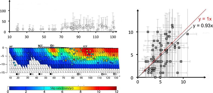
ance of these models, but it should be noted that the who showed the easternmost segment of the transformUchida Progress in Earth and Planetary Science (2019) 6:40 Page 14 of 21 Mendocino Fault Zone displays creep at about 65% of 1984 Morgan Hill earthquake (M6.2). They showed re- the long-term slip rate, and Rau et al. (2007) who esti- peating earthquakes occur preferentially in areas adja- mated 24.9–77.5 mm/year slip rates 10–22 km deep on cent to the coseismic rupture and the activity indicates the northern Longitudinal Valley fault in Taiwan, which accelerated slip and decay. In the case of the 1989 Loma are comparable to the GPS-derived slip rates of 47.5 ± Prieta earthquake (M6.9), the creep rate on the San An- 5.8 mm/year at similar depths. Also, Chen et al. (2008) dreas fault adjacent to the coseismic rupture increased suggested that along its northern half, the 30-km-long dramatically after the earthquake and fell back to its Chihshang fault is creeping at a rate of ~ 3 cm/year at interseismic rate in about 10 years. On the other hand, 7–23 km depth, Schmittbuhl et al. (2016) suggest that the nearly subparallel Sargent fault did not show an im- fault creep occurs in the Marmara Sea along the north mediate response (Turner et al. 2013). It is also interest- Anatolian fault, and Templeton et al. (2008) estimated ing that the creep of the two faults appears correlated, cumulative creep on several strike-slip faults in central suggesting a mutual driving force in the system. Other California over 21 years (Table 1). examples of postseismic deformation include the 2004 The time-dependent creep rate estimated from repeat- Parkfield earthquake (Mw6.0) (Khoshmanesh et al. 2015) ing earthquakes helps reveal the dynamic nature of slow and a large slow-slip transient following the 1998 earth- fault slip. Nadeau and McEvilly (2004) showed a quake near San Juan Bautista (Mw 5.1) (Taira et al. quasi-periodic occurrence of slow slip accelerations 2014) on either end of the creeping section of the San along a ~ 175-km-long section of the central San An- Andreas fault. As the fault surface surrounding these dreas fault. The transient events occurred both in con- two ruptures is generally accommodating slip by fault junction with and independent of transient slip from creep, effective moment release by afterslip appears to larger earthquakes. Recently, Turner et al. (2015), revised have exceeded that of their respective mainshocks. slip rate fluctuations with additional repeater data (1984–2011) and compared them with InSAR data Slow slip in Japan and other subduction zones (Fig. 11). They find that the slip rate fluctuates over ~ 2 Repeaters in subduction zones were first found in the year periods. The distribution of postseismic slip of northeastern Japan subduction zone. They enabled the major earthquakes is also evident from repeater data. estimation of the spatial variation of interplate creep Templeton et al. (2009) examined the distribution of rates beneath the sea (Igarashi et al. 2003; Matsuzawa et postseismic slip on the Calaveras fault following the al. 2002). The spatial heterogeneity of slow slip in Fig. 11 Periodic slip rate change observed along the San Andreas fault (after Turner et al. (2015)). The slip rate is denoted by color and in percent difference from the average long-term rate. Red and blue indicate slip rates higher or lower than the long-term average. White indicates higher uncertainty associated with fewer repeating earthquake sequences or with rapidly changing rates. White bars at the lower right show the spatial and temporal smoothing windows used. Thick and thin horizontal bars show the rupture extent and timing of The Loma Prieta (LP, in green) and Parkfield (PF, in red) earthquakes. Circles show earthquakes along the fault (M ≧ 3.5) that are scaled along with their magnitude (see scale at top left). The yellow highlighted trace shows the slip rate history (given in absolute terms) in the section from 85 to 95 km NW of PF
Uchida Progress in Earth and Planetary Science   (2019) 6:40                                                  Page 15 of 21

northeastern Japan also revealed strong coupling and an        al. (2005) and Uchida et al. (2009b) studied the afterslip
absence of repeaters in the maximum slip area of the           of the 2003 Tokachi-oki earthquake (M8.0) and its mi-
2011 M9.0 Tohoku-oki earthquake (Uchida and Matsu-             gration. They suggest that the migration of afterslip trig-
zawa 2011). Slow slip rates identified using repeaters re-     gered aftershocks and adjacent large earthquakes
vealed contrasts in interplate coupling off Kanto and          (Uchida et al. 2009b). In the case of the 2012 Haida
Tohoku, Japan where the overlying plates are different         Gwaii earthquake in the Queen Charlotte plate boundary
(Philippine Sea plate and Okhotsk plates) (Uchida et al.       zone, the mainshock on the subduction plate interface
2009a). Examples of estimates of spatial changes in sub-       triggered postseismic slip not only on the subduction
duction creep rate variation include Igarashi (2010) who       thrust but also on the strike-slip fault that accommo-
conducted a systematic search of repeaters around Japan        dates trench-parallel motion of the oblique subduction
and found variations of slip rate related to past large        in the area (Hayward and Bostock 2017).
earthquakes’ locations and spatial differences in plate           Quasi-periodic slow slip behavior similar to that ob-
convergence rates. Yamashita et al. (2012) found spatially     served on the San Andreas fault was also found along a
heterogeneous interplate coupling in the southwestern          ~ 900-km-long segment along the Japan and Kuril
Japan subduction zone and Yu (2013) found that inter-          trenches (Uchida et al. 2016b). Its periodicity varied
plate     coupling    is   mostly    weak     along    the     from 1 to 6 years, and slip accelerations often coincided
Tonga-Kermadec-Vanuatu subduction zone except for in           with or preceded clusters of large (M ≥ 5) earthquakes,
the northern section (15°–19° S) of the Tonga arc              including the 2011 M9 Tohoku-oki earthquake. The
(Table 1). These estimates of interplate coupling have         swarm-like activity pattern of small repeating earth-
contributed to the assessment of the potential for mega-       quakes that emerged before some of the largest earth-
thrust earthquakes.                                            quakes suggests that spontaneous slow-slip events are
   Temporal changes in slow slip rates in subduction           involved in the underlying aseismic loading process that
zones revealed that postseismic slip can be resolved for       drives episodic deformation transients and earthquakes.
smaller earthquakes than previously observed (e.g.,               Preseismic slow slip has been reported in several areas.
Uchida et al. 2003). Postseismic slip following earth-         Uchida et al. (2004) reported on the slow slip in the 3
quakes has been observed using repeating earthquakes           days, 1 week, and 8 months before three off-Sanriku,
for many subduction zone earthquakes including the             Japan M~ 7 earthquakes. For the 2011 Tohoku-oki
1994 Sanriku-oki earthquake (M7.6) (Uchida et al.              earthquake, the aftershocks of a M7.3 earthquake that
2004), the 2003 Tokachi-oki earthquake (M8.0) (Matsu-          occurred 2 days before the mainshock contained many
bara et al. 2005), the 2004 Sumatra earthquake (M9.2)          repeating earthquakes suggesting the occurrence of slow
(Yu et al. 2013), the 2005 Nias earthquake (M8.6) (Yu et       slip (Kato et al. 2012; Uchida and Matsuzawa 2013)
al. 2013), the 2011 Tohoku-oki earthquake (Mw 9.0)             (Fig. 12a, Fig. 13a). Kato et al. (2012) showed that re-
(Uchida and Matsuzawa 2013), and the 2012 Nicoya               peaters are included in the seismicity that migrated twice
earthquake (Mw7.6) (Yao et al. 2017) (Table 1). These          in the direction of the hypocenter of the mainshock
results provide independent and useful estimations of          (Fig. 13a). Such indications of slow slip on time scales of
postseismic slip complementary to those obtained from          days to weeks were also found for the 2014 Iquique
geodetic data. Figure 12e, f shows an example of variable      earthquake (M8.1) (Kato and Nakagawa 2014; Meng et
afterslips of the 2011 Tohoku-oki earthquake that de-          al. 2015), a 2016 Mw 6.0 earthquake in central Italy
pends on the location on the plate boundary. In general,       (Vuan et al. 2017) and the 2017 Valparaiso earthquake
the regions close to the Tohoku-oki earthquake’s rupture       in Chile (Ruiz et al. 2017). On the other hand, Mavrom-
area show rapid afterslip (Fig. 12e) while distant places      matis et al. (2015) and Uchida and Matsuzawa (2013)
show small or delayed afterslip (Fig. 12f ). The rupture       showed long-term slip rates increased for several years
area of the Tohoku-oki earthquake shows no afterslip           to a decade around the seismic slip area of the 2011
(Fig. 12d). The Tohoku-oki earthquake also speeds up           Tohoku-oki earthquake (Fig. 13b). Since interplate
slip on the adjacent plate boundary in the Kanto area          non-steady slow slip produces transient stress increases
(regions 16 and 17 in Fig. 12) where there is a different      in the adjacent areas (Mazzotti and Adams 2004; Obara
overlying plate (Philippine Sea plate) than in the source      and Kato 2016), it is important to monitor slow slip
area (Okhotsk plate) (Uchida et al. 2016a). Nomura et al.      from repeating earthquakes.
(2017) studied 13 major earthquakes in the northeastern
Japan subduction zone using the same method and ob-            Toward a better use of repeating earthquake data for
tained a relationship of mainshock magnitude with loga-        estimating slow fault slip
rithms of the duration and total moment of postseismic         Repeater data provide estimates of slow fault slip that
slip. The results show general proportional relationship       are independent from geodetic data. Comparisons of
and illuminated deviations for each event. Matsubara et        slow slip based on geodetic data and on repeaters have
You can also read