THE TRANSFORMER EARTHQUAKE ALERTING MODEL: A NEW VERSATILE APPROACH TO EARTHQUAKE EARLY WARNING - arXiv.org
←
→
Page content transcription
If your browser does not render page correctly, please read the page content below
T HE TRANSFORMER EARTHQUAKE ALERTING MODEL : A NEW
                                                        VERSATILE APPROACH TO EARTHQUAKE EARLY WARNING

                                                                        Jannes Münchmeyer1,2,∗ , Dino Bindi1 , Ulf Leser2 , Frederik Tilmann1,3
arXiv:2009.06316v4 [physics.geo-ph] 11 Jan 2021

                                                                                1
                                                                                  Deutsches GeoForschungsZentrum GFZ, Potsdam, Germany
                                                                         2
                                                                           Institut für Informatik, Humboldt-Universität zu Berlin, Berlin, Germany
                                                                    3
                                                                      Insitut für geologische Wissenschaften, Freie Universität Berlin, Berlin, Germany
                                                                      ∗
                                                                        To whom correspondence should be addressed: munchmej@gfz-potsdam.de

                                                                                                        January 12, 2021

                                                                                                         A BSTRACT
                                                           Earthquakes are major hazards to humans, buildings and infrastructure. Early warning methods
                                                           aim to provide advance notice of incoming strong shaking to enable preventive action and mitigate
                                                           seismic risk. Their usefulness depends on accuracy, the relation between true, missed and false alerts,
                                                           and timeliness, the time between a warning and the arrival of strong shaking. Current approaches
                                                           suffer from apparent aleatoric uncertainties due to simplified modelling or short warning times. Here
                                                           we propose a novel early warning method, the deep-learning based transformer earthquake alerting
                                                           model (TEAM), to mitigate these limitations. TEAM analyzes raw, strong motion waveforms of an
                                                           arbitrary number of stations at arbitrary locations in real-time, making it easily adaptable to changing
                                                           seismic networks and warning targets. We evaluate TEAM on two regions with high seismic hazard,
                                                           Japan and Italy, that are complementary in their seismicity. On both datasets TEAM outperforms
                                                           existing early warning methods considerably, offering accurate and timely warnings. Using domain
                                                           adaptation, TEAM even provides reliable alerts for events larger than any in the training data, a
                                                           property of highest importance as records from very large events are rare in many regions.

                                                  1    Introduction

                                                  The concept of earthquake early warning has been around for over a century, but the necessary instrumentation and
                                                  methodologies have only been developed in the last three decades [1, 2]. Early warning systems aim to raise alerts
                                                  if shaking levels likely to cause damage are going to occur. Existing methods split into two main classes: source
                                                  estimation based and propagation based. The former, like EPIC [3] or FINDER [4], estimate the source properties of an
                                                  event, i.e., its location or fault extent and magnitude, and then use a ground motion prediction equation (GMPE) to
                                                  infer shaking at target sites. They provide long warning times, but incur a large apparent aleatoric uncertainty due to
                                                  simplified assumptions in the source estimation and in the GMPE [5]. Propagation based methods, like PLUM [5],
                                                  infer the shaking at a given location from measurements at nearby seismic stations. Predictions are more accurate, but
                                                  warning times are reduced, as warnings require measurements of strong shaking at nearby stations [6].
                                                  Recently, machine learning methods, particularly deep learning methods, have emerged as a tool for fast assessment of
                                                  earthquakes. Under certain circumstances, they led to improvements in various tasks, e.g., estimation of magnitude
                                                  [7, 8], location [9, 10] or peak ground acceleration (PGA) [11]. Nonetheless, no existing method is applicable to
                                                  early warning because they lack real-time capabilities, instead requiring fixed waveform windows after the P arrival.
                                                  Furthermore, the existing methods are restricted in terms of their input stations, as they use either a single seismic station
                                                  as input [7, 8] or a fixed set of seismic stations, that needs to be defined at training time [9, 11, 12]. While single station
                                                  approaches miss out on a considerable amount of information obtainable from combining waveforms from different
                                                  sources, fixed stations approaches have limited adaptability to changing networks. The latter is of particular concern as
                                                  for large, dense networks the stations of interest, i.e., the stations closest to an event, will change on a per-event basis.
                                                  Finally, existing methods systematically underestimate the strongest shaking and the highest magnitudes, as these are
The transformer earthquake alerting model

Figure 1: Map of the station (left) and event (right) distribution in the Japan dataset. Stations are shown as black
triangles, events as dots. The event color encodes the event magnitude. There are ∼20 additional events far offshore,
which are outside the displayed map region in the catalog.

rare and therefore underrepresented in the training data (Fig. 6, 8 in [11], Fig. 3, 4 in [8]). However, early warning
systems must also be able to provide reliable warnings for earthquakes larger than any previously seen in a region.
Here, we present the transformer earthquake alerting model (TEAM), a deep learning method for early warning,
combining the advantages of both classical early warning strategies while avoiding the deficiencies of prior deep
learning approaches. We evaluate TEAM on two data sets from regions with high seismic hazard, namely Japan and
Italy. Due to their complementary seismicity, this allows to evaluate the capabilities of TEAM across scenarios. We
compare TEAM to two state-of-the-art warning methods, of which one is prototypical for source based warning and
one for propagation based warning.

2     Data and Methods

2.1   Data

For our study we use two nation scale datasets from highly seismically active regions with dense seismic networks,
namely Japan (13,512 events, years 1997-2018, Figure 1) and Italy (7,055 events, years 2008-2019, Figure 2). Their
seismicity is complementary, with predominantly subduction plate interface or Wadati-Benioff zone events for Japan,
many of them offshore, and shallow, crustal events for Italy. We split both datasets into training, development and test
sets with ratios of 60:10:30. We employ an event-wise split, i.e., all records for a particular event will be assigned to the
same subset. We do not explicitly split station-wise but due to temporary deployments there are a few stations in the
test set which have no records in the training set (Figure 2). We use the training set for model training, the development
set for model selection, and the test set only for the final evaluation. We split the Japan dataset chronologically, yielding
the events between August 2013 and December 2018 as test set. For Italy, we test on all events in 2016, as these are of
particular interest, encompassing most of the central Italy sequence with the MW =6.2 and Mw =6.5 Norcia events [13].
Especially the latter event is notably larger than any in the training set (Mw = 6.1 L’Aquila event in 2007), thereby
challenging the extrapolation capabilities of TEAM.
Both datasets consist of strong motion waveforms. For Japan each station comprises two sensors, one at the surface and
one borehole sensor, while for Italy only surface recordings are available. As the instrument response in the frequency
band of interest is flat, we do not restitute the waveforms, but only apply a gain correction. This has the advantage that
it can trivially be done in real-time. The data and preprocessing are further described in the supplement text S1.

                                                             2
The transformer earthquake alerting model

Figure 2: Map of the station (left) and event (right) distribution in the Italy dataset. Stations present in the training set
are shown as black triangles, while stations only present in the test set are shown as yellow triangles. Events are shown
as dots with the color encoding the event magnitude. All events with magnitudes above 5.5 are shown as stars. The red
stars indicate large training events, while the yellow stars indicate large test events. The inset shows the central Italy
region with intense seismicity and high station density in the test set. Moment magnitudes for the largest test events are
given in the inset.

2.2   The transformer earthquake alerting model

The early warning workflow with TEAM encompasses three separate steps (Figure 3): event detection, PGA estimation
and thresholding. We do not further consider the event detection task here, as it forms the base of all methods discussed
and affects them similarly. The PGA estimation, resulting in PGA probability densities for a given set of target locations,
is the heart of TEAM and described in detail below. In the last step, thresholding, TEAM issues warnings for each target
locations where the predicted exceedance probability p for fixed PGA thresholds surpasses a predefined probability α.
TEAM conducts end-to-end PGA estimation: its input are raw waveforms, its output predicted PGA probability
densities. There are no intermediate representations in TEAM that warrant an immediate geophysical interpretation.
The PGA assessment can be subdivided into three components: feature extraction, feature combination, and density
estimation (Figure S1). Input to TEAM are three, respectively six (3 surface, 3 borehole), component waveforms at 100
Hz sampling rate from multiple stations and the corresponding station coordinates. Furthermore, the model is provided
with a set of output locations, at which the PGA should be predicted. These can be anywhere within the spatial domain
of the model and need not be identical with station locations in the training set.
TEAM extracts features from input waveforms using a convolutional neural network (CNN). The feature extraction is
applied separately to each station, but is identical for all stations. CNNs are well established for feature extraction from
seismic waveforms, as they are able to recognize complex features independent of their position in the trace. On the
other hand, CNN based feature extraction usually requires a fixed input length, inhibiting real-time processing. We
allow real-time processing through the alignment of the waveforms and zero-padding: we align all input waveforms in
time i.e., all start at the same time t0 and end at the same time t1 . We define t0 to be 5 s before the first P wave arrival at
any station, allowing the model to understand the noise characteristics. For t1 we use the current time, i.e., the amount
of available waveforms. We obtain constant length input, by padding all waveforms after t1 with zeros up to a total
length of 30 s. The feature extraction is described in more detail in supplementary text S2.
TEAM combines the feature vectors and maps them to representations at the targets using a transformer [14]. Trans-
formers are attention-based neural networks for combining information from a flexible number of input vectors in a
learnable way. To encode the location of the recording stations as well as of the prediction targets, we use sinusoidal
vector representations. For input stations, we add these representations component-wise to the feature vectors, for
target stations we directly use them as inputs to the transformer. This architecture, processing a varying number of
inputs, together with the explicitly encoded locations, allows TEAM to handle dynamically varying sets of stations and

                                                               3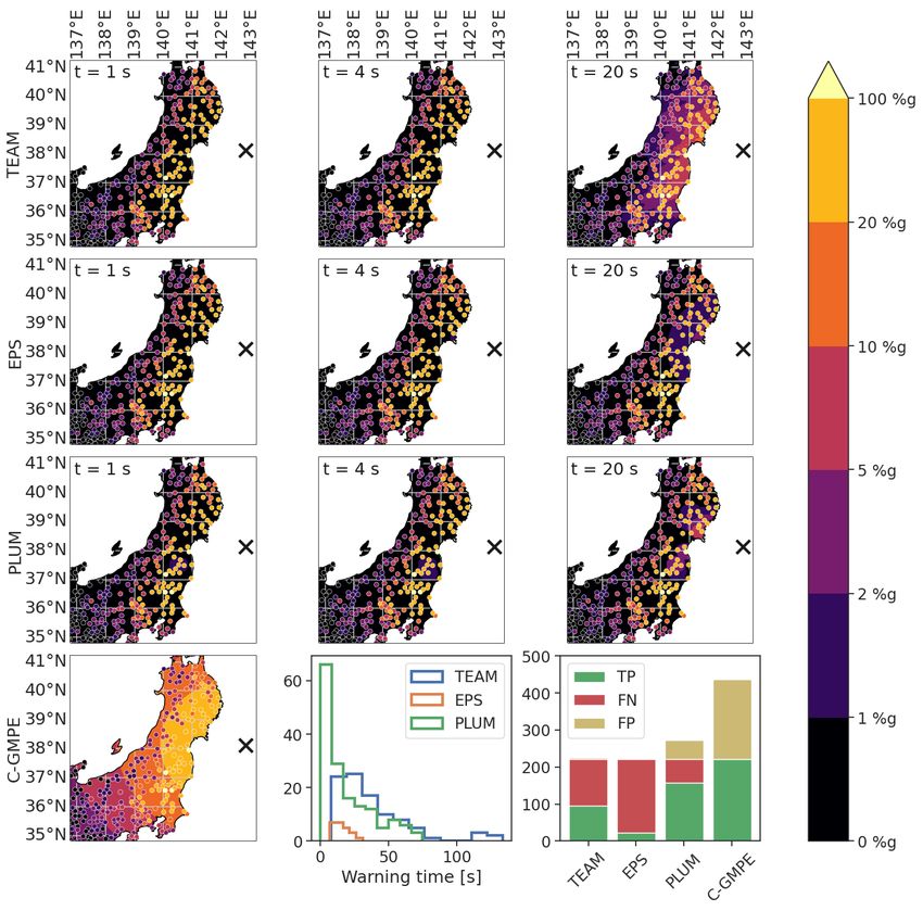
The transformer earthquake alerting model

Figure 3: Schematic view of TEAM’s early warning workflow for the October 2016 Norcia event (Mw = 6.5) 2.5 s
after the first P wave pick (∼3.5 s after origin time). a. An event is detected through triggering at multiple seismic
stations. The waveform colors correspond to the stations highlighted with orange to magenta outlines. The circles
indicate the approximate current position of P (dashed) and S (solid) wavefronts. b. TEAM’s input are raw waveforms
and station coordinates; it estimates probability densities for the PGA at a target set. A more detailed TEAM overview
is given in Figure S1. c. The exceedance probabilities for a fixed set of PGA thresholds are calculated based on the
estimated PGA probability densities. If the probability exceeds a threshold α, a warning is issued. The figure visualizes
a 10%g PGA level with α = 0.4, resulting in warnings for the stations highlighted. The colors correspond to the
stations with green outlines in a. d. The real-time shake map shows the highest PGA levels for which a warning is
issued. Stations are colored according to their current warning level. The table lists all stations for which warnings have
already been issued.

targets. The transformer returns one vector for each target representing predictions at this target. Details on the feature
combinations can be found in supplementary text S3.
From each of the vectors returned by the transformer, TEAM calculates the PGA predictions at one target. Similar to
the feature extraction, the PGA prediction network is applied separately to each target, but is identical for all targets.
TEAM uses mixture density networks [15] returning Gaussian mixtures, to computes PGA densities. Gaussian mixtures
allow TEAM to predict more complex distributions and better capture realistic uncertainties than a point estimate or a
single Gaussian. The full specifications for the final PGA estimation are provided in supplementary text S4.
TEAM is trained end-to-end using a negative log-likelihood loss. To increase the flexibility of TEAM and allow for
real-time processing, we use training data augmentation. We randomly select the stations used as inputs and targets in
each training iteration. In addition, again in each training iteration, we randomly replace all waveforms after a time t
with zeros, matching the input representation of real time data, to train TEAM for real-time application. These data
augmentations as well as the complete training procedure are further described in supplementary text S5.
To mitigate the systematic underestimation of high PGA values observed in previous machine learning models, TEAM
oversamples large events and PGA targets close to the epicenter during training, which reduces the inherent bias in
data towards smaller PGAs. When learning from small catalogs or when applied to regions where events substantially
larger than all training events can be expected, e.g., because of known locked fault patches or historic records, TEAM
additionally can use domain adaptation. To this end the training procedure is modified to include large events from
other regions that are similar to the expected events in the target region. While records from those events will differ in
certain aspects, e.g., site responses or the exact propagation patterns, other aspects, e.g., the average extent of strong

                                                            4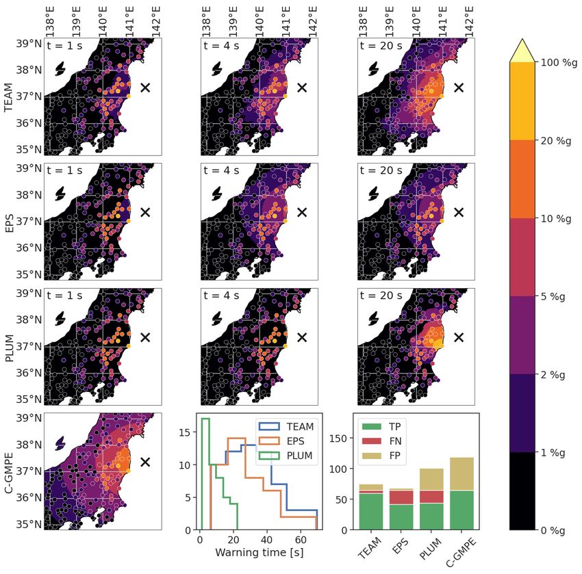
The transformer earthquake alerting model
shaking or the duration of events of a certain size, will mostly be independent of the region in question. The domain
adaptation aims to enable the model to transfer the region immanent aspects of large events, at the cost of a certain
blurring of the specific regional aspects of the target region. TEAM aims to mitigate the blurring of regional aspects by
the choice of training procedure.
Our Italy dataset is an example of this situation. Accordingly, TEAM applies domain adaptation to this case: It first
trains a joint model using data from Japan and from Italy, which is then fine-tuned using the Italy data on its own,
except for the addition of a few large, shallow, onshore events from Japan. We chose these events, as for Italy one also
expects large, shallow, crustal events due to its tectonic setting and earthquake history. As we use events from Italy in
both training steps and in particular in the second step the overwhelming number of events are from Italy, we expect
that this scheme only results in a small degradation in the modelling of the regional specifics of the Italy region.
2.3 Baselines
We compare TEAM to two state-of-the-art early warning methods, one using source estimation and one propagation
based. As source estimation based method we use the estimated point source approach (EPS), which estimates
magnitudes from peak displacement during the P-wave onset [16] and then applies a GMPE [17] to predict the PGA.
For simplicity, our implementation assumes knowledge of the final catalog epicentre, which is impossible in real-time,
leading to overoptimistic results for EPS. As propagation based method we chose an adaptation of PLUM [5], which
issues warnings if a station within a radius r of the target exceeds the level of shaking. In contrast to the original PLUM,
which operates on the Japanese seismic intensity scale, IJM A [18], our adaptation applies the concept of PLUM to PGA,
thereby making it comparable to the other approaches. Whereas IJM A is also a measure of the strongest acceleration
and is thus strongly correlated with PGA, it considers a narrower frequency band and imposes a mimum duration of
strong shaking. As such, although the perfomance might vary slightly for our PLUM-like approach compared to the
original PLUM, it still exhibits its key features, in particular the effects of the localized warning strategy. Additionally
we apply the GMPE used in EPS to catalog location and magnitude as an approximate upper accuracy bound for point
source algorithms (Catalog-GMPE or C-GMPE). C-CMPE is a theoretical bound that can not be realized in real-time.
It can be considered as an estimate of the modeling error for point source approaches. A detailed description of the
baseline methods can be found in supplementary text S6.
3 Results
3.1 Alert performance
We compare the alert performance of all methods for PGA thresholds from light (1%g) to very strong (20%g) shaking,
regarding precision, the fraction of alerts actually exceeding the PGA threshold, and recall, the fraction of issued
alerts among all cases where the PGA threshold was exceeded [19, 20]. Precision and recall trade-off against each
other depending on α. While the PGA predictions of TEAM, EPS and the C-GMPE are probabilistic, the thresholding
transforms the predictions into alerts or non-alerts. The probability distribution describes the uncertainty of the models,
e.g., for the GMPE the apparent aleatoric uncertainty from aspects not accounted for, which makes false and missed
alerts inevitable. The threshold value controls the trade-off between both types of errors, and its appropriate value
will depend on user needs, specifically the costs associated with false and missed alerts. Therefore, to analyze the
performance of the models across different user requirements, we look at the precision recall curves for different
thresholds α. In addition to precision and recall, we use two summary metrics: F1 score, the harmonic mean of
precision and recall, and AUC, the area under the precision recall curve. The evaluation metrics and full setup of the
evaluation are defined in detail in supplement text S7.
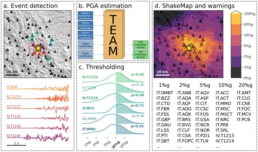
TEAM outperforms both EPS and the PLUM-like approach for both datasets and all PGA thresholds, indicated by the
precision-recall-curves of TEAM lying to the top-right of the baseline curves (Figure 4a). For any baseline method
configuration, there is a TEAM configuration surpassing it both in precision and in recall. Improvements are larger for
Japan, but still substantial for Italy. To compare the performance at fixed α, we selected α values yielding the highest
F1 score separately for each PGA threshold and method. Again, TEAM outperforms both baselines on both datasets,
irrespective of the PGA level (Figure 4b). Performance statistics in numerical form are available in tables S1 and S2.
All methods degrade with increasing PGA levels, particularly for Japan. This degradation is intrinsic to early warning
for high thresholds due to the very low prior probability of strong shaking [6, 20, 19]. Furthermore, shortage of training
data with high PGA values results in less well constrained model parameters.
Using domain adaptation techniques, TEAM copes well with the Italy data, even though the largest test event (Mw = 6.5)
is significantly larger than the largest training event (Mw = 6.1), and three further test events have MW ≥ 5.8. To
assess the impact of this technique, we compared TEAM’s results to a model trained without it (Figures S2, S3).
5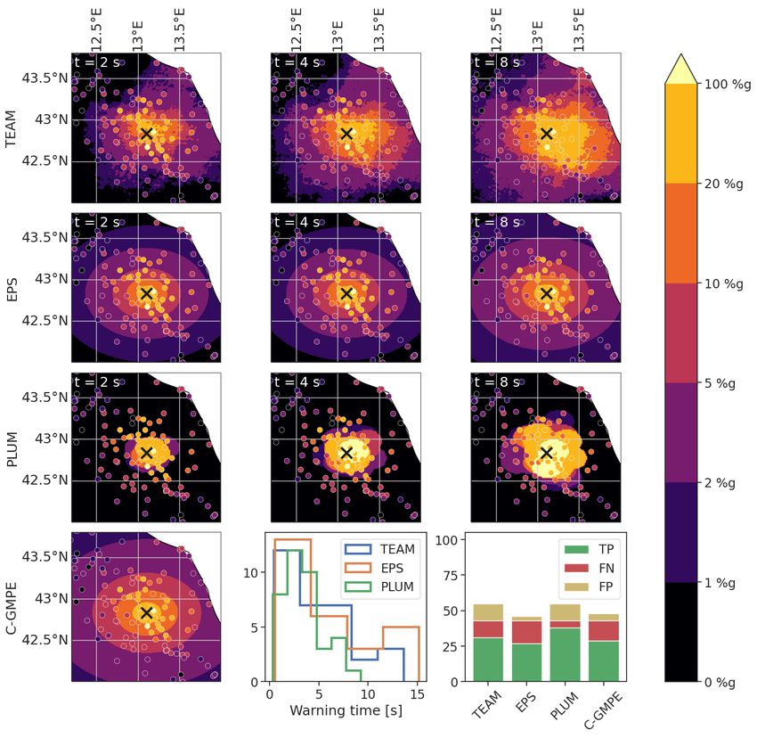
The transformer earthquake alerting model

Figure 4: Warning statistics for the three early-warning models (TEAM, EPS, PLUM) for the Japan and Italy datasets.
In addition, statistics are provided for C-GMPE, which can only be evaluated post-event due to its reliance on catalog
magnitude and location. a. Precision and recall curves across different thresholds α = 0.05, 0.1, 0.2, . . . , 0.8, 0.9, 0.95.
As the PLUM-like approach has no tuning parameter, its performance is shown as a point. Enlarged markers show
the configurations yielding the highest F1 scores. Numbers in the corner give the area under the precision recall curve
(AUC), a standard measure quantifying the predictive performance across thresholds. b. Precision, recall and F1 score
at different PGA thresholds using the F1 optimal value α. Threshold probabilities α were chosen independently for
each method and PGA threshold. c. Number of events and traces exceeding each PGA threshold for training and test
set. Training set numbers include development events and show the numbers before oversampling is applied. For Italy
training and test event curve are overlapping due to similar numbers of events.

                                                              6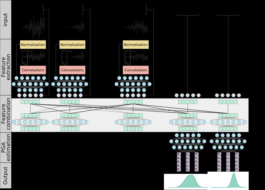
The transformer earthquake alerting model

Figure 5: Warning time statistics. a. Area under the precision recall curve for different minimum warning times. All
alerts with shorter warning times are counted as false negatives. b. Warning time histograms showing the distribution
true alerts across distances for the different methods. Please note that the total number of true alerts differs by method
and is not shown in this subplot. Therefore the values of different methods can not be directly compared, but only the
differences in the distributions. TEAM and EPS are shown at F1-optimal α, chosen separately for each threshold and
method. Warning time dependence on hypocentral distance is shown in Figure S4.

While for low PGA thresholds differences are small, at high PGA levels they grow to more than 20 points F1 score.
Interestingly, for large events, TEAM strongly outperforms TEAM without domain adaptation even for low PGA
thresholds. This shows that domain adaptation does not only allow the model to predict higher PGA values, but also to
accurately assess the region of lighter shaking for large events. Domain adaptation therefore helps TEAM to remain
accurate even for events quite far from the training distribution.

3.2   Warning times

In application scenarios, a user will usually require a certain warning time, which is the time between issuing of
the warning and first exceedance of the level of shaking, as this time is necessary for taking action. As the previous
evaluation considered prediction accuracy irrespective of the warning time, we now compare the methods while
imposing a certain minimum warning time. Actually, TEAM consistently outperforms both baselines across different
required warning times and irrespective of the PGA threshold (Figure 5a). While the margin for TEAM compared to
the baselines is smaller for Italy than for Japan, TEAM shows consistently strong performance across different warning
times. In contrast, EPS performs clearly worse at short warning times, the PLUM-based approach at longer warning
times. The latter is inherent to the key idea of PLUM and makes the method only competitive at high PGA thresholds,
where potential maximum warning times are naturally short due to the proximity between stations with strong shaking
and the epicenter [21]. We further note that while the PLUM-like approach shows slightly higher AUC than TEAM for
short warning times at 20 %g, this is only a hypothetical result. As PLUM does not have a tuning parameter between
precision and recall, this performance can actually only be realised for a specific precision/recall threshold, where it
performs slightly superior to TEAM (Figure 4a bottom right).

                                                            7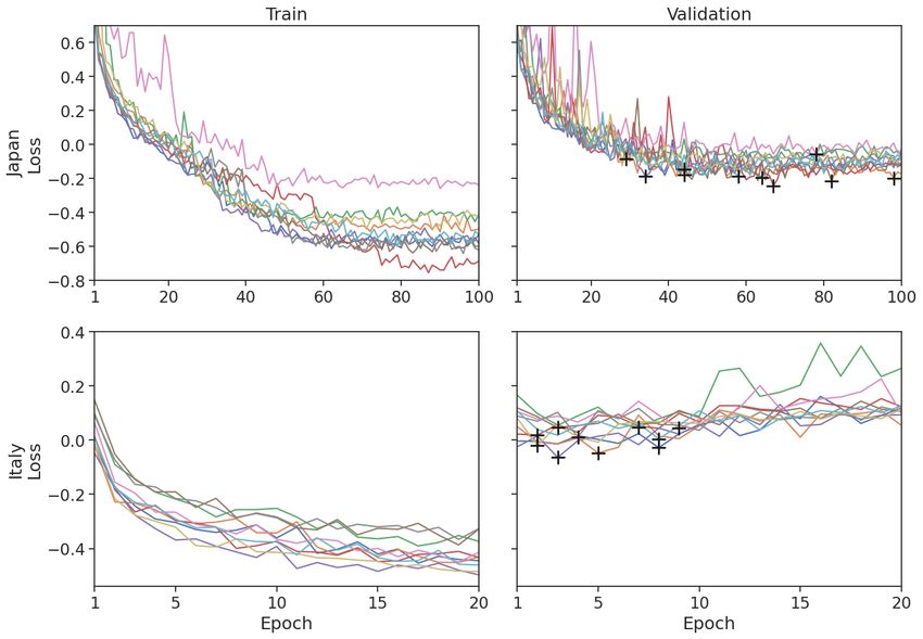
The transformer earthquake alerting model

Warning times depend on α: a lower α value naturally leads to longer warning times but also to more false positive
warnings. At F1-optimal thresholds α, EPS and TEAM have similar warning time distributions (Figure 5b, Table S3),
but lowering α leads to stronger increases in warning times for TEAM. For instance, at 10%g, lowering α from 0.5 to
0.2 increases average warning times of TEAM by 2.3 s/1.2 s (Japan/Italy), but only by 1.1 s/0.1 s for EPS. Short times
as measured here are critical in real applications: First, they reduce the time available for counter measures. Second,
real warning times will be shorter than reported here due to telemetry and compute delays. However, compute delays
for TEAM are very mild: analysing the Norcia event (25 input stations, 246 target sites) for one time step took only
0.15 s on a standard workstation using non-optimized code.

4     Discussion
4.1   Calibration of probabilities

Even though TEAM and EPS give probabilistic predictions, it is not clear whether these predictions are well-calibrated,
i.e., if the predicted confidence values actually correspond to observed probabilities. Calibrated probabilities are
essential for threshold selection, as they are required to balance expected costs of taking action versus expected costs of
not taking action. We note that while good calibration is a necessary condition for a good model, it is not sufficient, as a
model constantly predicting the marginal distribution of the labels would be always perfectly calibrated, yet not very
useful.
To assess the calibration, we use calibration diagrams (Figures S9 and S10) for Japan and Italy at different times after
the first P arrival. These diagrams compare the predicted probabilities to the actually observed fraction of occurrences.
In general, both models are well calibrated, with a slightly better calibration for TEAM. Calibration is generally better
for Japan, where only EPS is slightly underconfident at earlier times for the highest PGA thresholds. For Italy, EPS
is generally slightly overconfident, while TEAM is well calibrated, except for a certain overconfidence at 20%g. We
suspect that the worse calibration for the largest events is caused by the domain adaptation strategy, but the better
performance in terms of accuracy clearly weighs out this downside of domain adaptation.

4.2   Insights into the transformer earthquake alerting model

We analyze differences between the methods using one example event from each dataset (Japan: Figure 6, Italy: Figure
S5). All methods underestimate the shaking in the first seconds (left column Figures 6, S5). However, TEAM is
the quickest to detect the correct extent of the shaking. Additionally, it estimates even fine-grained regional shaking
details in real-time (middle and right columns). In contrast, shake maps for EPS remain overly simplified due to the
assumptions inherent to GMPEs (right column and bottom left panel). For the Japan example, even late predictions of
EPS understimate the shaking, due to an underestimation of the magnitude. The PLUM-based approach produces very
good PGA estimates, but exhibits the worst warning times.
Notably, TEAM predictions at later times correspond even better to the measured PGA than C-GMPE estimates,
although these are based on the final magnitude (top right and bottom left panels). For the Japan data, this is not only
the case for the example at hand, but also visible in Figure 4, showing higher accuracy of TEAM’s prediction compared
to C-GMPE for all thresholds except 20%g on the full Japan dataset. We assume TEAM’s superior performance is
rooted in both global and local aspects. Global aspects are the abilities to exploit variations in the waveforms, e.g.,
frequency content, to model complex event characteristics, such as stress drop, radiation pattern or directivity, and to
compare to events in the training set. Local aspects include understanding regional effects, e.g., frequency dependent
site responses, and the ability to consider shaking at proximal stations. We note that for our Italy experiments, the
modelling of local aspects resulting from regional characteristics might be slightly degraded by the domain adaptation.
However, the first-order propagation effects such as, e.g., amplitude decay due to geometric spreading, are similar
between regions and therefore not negatively affected by the domain adaptation. In conclusion, combining a global
event view with propagation aspects, TEAM can be seen as a hybrid model between source estimation and propagation.

4.3   TEAM performance on the Tohoku sequence

We evaluated TEAM for Japan on a chronological train/dev/test split, as this split ensures the evaluation closest to the
actual application scenario. On the other hand, this split put the M = 9.1 Tohoku event in March 2011 into the training
set. To evaluate the performance for this very large event and its aftershocks, we trained another TEAM instance using
the year 2011 as test set and the remainder of the data for training and validation. Figure 7 shows the precision recall
curves for the chronological split and the year 2011 as test set. In general, the performance of all models stays similar
when evaluated on the alternative split. A key difference between the curves is, that TEAM, in particular for high
PGA thresholds, does not reach similar levels of recall for 2011 as for the chronological split, while achieving higher

                                                             8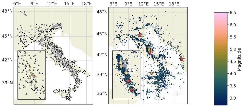
The transformer earthquake alerting model

Figure 6: Scenario analysis of the 22nd November 2016 MJ = 7.4 Fukushima earthquake, the largest test event located
close to shore. Maps show the warning levels for each method (top three rows) at different times (shown in the corner,
t = 0 s corresponds to P arrival at closest station). Dots represent stations and are colored according to the PGA
recorded during the full event, i.e., the prediction target. The bottom row shows (left to right), the catalog based GMPE
predictions, the warning time distributions, and the true positives (TP), false negatives (FN) and false positives (FP) for
each method, both at a 2%g PGA threshold. EPS and GMPE shake map predictions do not include station terms, but
they are included for the bottom row histograms.

                                                            9
The transformer earthquake alerting model

Figure 7: Precision recall curves for the Japanese dataset using the chronological split (top) and using the events in
2011 as test set (bottom). The year 2011 contains the Mw = 9.1 Tohoku event as well as its aftershocks.

precision. As we will describe in the next paragraph, this trend probably results from a tendency to underestimate true
PGA amplitudes, which will naturally reduce recall and boost precision. Nevertheless, the performance of TEAM
as quantified by the AUC actually improves, and significantly so for the highest thresholds. We suspect that this
tendency for underestimation is either caused by the higher number of large events in the 2011 test set compared to the
chronological split, or by the lower number of high PGA events in the training set without 2011.
Figure S6 presents a scenario analysis for the Tohoku event. All models underestimate the event considerably, with the
strongest underestimation for the EPS method. Even 20 s after the first P wave arrival, all methods underestimate both
the severity and the extent of shaking. Do to its localized approach, the PLUM-based model achieves the highest number
of true warnings, albeit at short warning times and a certain number of false positives, which due to the underestimation
are totally absent from TEAM and EPS predictions. The performance of both EPS and TEAM is likely degraded by the
slow onset of the Tohoku event as described by [22]. According to [22] the main subevent with a displacement of 36 m
only initiated 20 s after the onset of the Tohoku event. Therefore only the first P waves for EPS or at most the first 25 s
of waveforms for TEAM is most likely insufficient to correctly estimate the size of the Tohoku event.
For Italy, we showed that underestimation for large events can be mitigated using transfer learning. However, the
Tohoku event clearly shows the limitations of this strategy, as nearly no training data for events of comparable size
are available, even when using events across the globe. Therefore, for the largest events alternative strategies need to
be developed, e.g., training using simulated data. Furthermore, the 25 s of waveforms used by TEAM in the current
implementation may, for a very large event, not capture the largest subevent. While we decided to use only 25 s of event
waveforms, as there is only insufficient training data of longer events, this window could be extended when developing
training strategies and models for the largest events.

5   Conclusion

In this study we presented the transformer earthquake alerting model (TEAM). TEAM outperforms existing early
warning methods in terms of both alert performance and warning time. Using a flexible machine learning model, TEAM
is able to extract information about an event from raw waveforms and leverage the information to model the complex
dependencies of ground motion. We point out two further aspects that make TEAM appealing to users. First, TEAM
can adapt to various user requirements by combining two thresholds, one for shake level and one for the exceedance
probability. As TEAM outputs probability density functions over the PGA, these thresholds can easily be adjusted by
individual users on the fly, e.g., by setting sliders in an early warning system. Second, deep learning models typically
exhibit large performance improvements from larger training datasets [23] due to the high number of model parameters.
In our study this reflects in the better performance on the twofold larger Japan dataset. This indicates that TEAM’s
performance can be improved just by collecting more comprehensive catalogs, which happens automatically over time.

                                                            10
The transformer earthquake alerting model
Acknowledgements
We thank the National Research Institute for Earth Science and Disaster Resilience (NIED) for providing the catalog and
waveform data for our Japan dataset. We thank the Istituto Nazionale di Geofisica e Vulcanologia and the Dipartimento
della Protezione Civile for providing the catalog and waveform data for our Italy dataset. J. M. acknowledges the
support of the Helmholtz Einstein International Berlin Research School in Data Science (HEIBRiDS). We thank Matteo
Picozzi for discussions on earthquake early warning that helped improve the study design. We thank Hiroyuki Goto and
an anonymous reviewer for their comments which helped to improve the manuscript. An implementation of TEAM and
the baselines is available at https://github.com/yetinam/TEAM. The Italy dataset has been published as [24]. The
Japan dataset can be obtained using the scripts in the code repository.
References
[1] R. M. Allen, P. Gasparini, O. Kamigaichi, and M. Bose. The Status of Earthquake Early Warning around the
World: An Introductory Overview. Seismological Research Letters, 80(5):682–693, September 2009.
[2] Richard M. Allen and Diego Melgar. Earthquake Early Warning: Advances, Scientific Challenges, and Societal
Needs. Annual Review of Earth and Planetary Sciences, 47(1):361–388, 2019.
[3] Angela I. Chung, Ivan Henson, and Richard M. Allen. Optimizing Earthquake Early Warning Performance:
ElarmS-3. Seismological Research Letters, 90(2A):727–743, March 2019.
[4] M. Böse, D. E. Smith, C. Felizardo, M.-A. Meier, T. H. Heaton, and J. F. Clinton. FinDer v.2: Improved
real-time ground-motion predictions for M2–M9 with seismic finite-source characterization. Geophysical Journal
International, 212(1):725–742, January 2018.
[5] Yuki Kodera, Yasuyuki Yamada, Kazuyuki Hirano, Koji Tamaribuchi, Shimpei Adachi, Naoki Hayashimoto,
Masahiko Morimoto, Masaki Nakamura, and Mitsuyuki Hoshiba. The Propagation of Local Undamped Motion
(PLUM) Method: A Simple and Robust Seismic Wavefield Estimation Approach for Earthquake Early WarningThe
Propagation of Local Undamped Motion (PLUM) Method. Bulletin of the Seismological Society of America,
108(2):983–1003, April 2018.
[6] Men-Andrin Meier, Yuki Kodera, Maren Böse, Angela Chung, Mitsuyuki Hoshiba, Elizabeth Cochran, Sarah
Minson, Egill Hauksson, and Thomas Heaton. How Often Can Earthquake Early Warning Systems Alert Sites
With High-Intensity Ground Motion? Journal of Geophysical Research: Solid Earth, 125(2):e2019JB017718,
2020.
[7] Anthony Lomax, Alberto Michelini, and Dario Jozinović. An Investigation of Rapid Earthquake Characteriza-
tion Using Single-Station Waveforms and a Convolutional Neural Network. Seismological Research Letters,
90(2A):517–529, 2019.
[8] S. Mostafa Mousavi and Gregory C. Beroza. A Machine-Learning Approach for Earthquake Magnitude Estimation.
Geophysical Research Letters, 47(1):e2019GL085976, 2020.
[9] Marius Kriegerowski, Gesa M. Petersen, Hannes Vasyura-Bathke, and Matthias Ohrnberger. A Deep Convolutional
Neural Network for Localization of Clustered Earthquakes Based on Multistation Full Waveforms. Seismological
Research Letters, 90(2A):510–516, 2019.
[10] S. Mostafa Mousavi and Gregory C. Beroza. Bayesian-Deep-Learning Estimation of Earthquake Location from
Single-Station Observations. arXiv:1912.01144 [physics], December 2019.
[11] Dario Jozinović, Anthony Lomax, Ivan Štajduhar, and Alberto Michelini. Rapid prediction of earthquake ground
shaking intensity using raw waveform data and a convolutional neural network. Geophysical Journal International,
222(2):1379–1389, 2020.
[12] Ryota Otake, Jun Kurima, Hiroyuki Goto, and Sumio Sawada. Deep Learning Model for Spatial Interpolation of
Real-Time Seismic Intensity. Seismological Research Letters, 91(6):3433–3443, November 2020.
[13] Mauro Dolce and Daniela Di Bucci. The 2016–2017 Central Apennines Seismic Sequence: Analogies and
Differences with Recent Italian Earthquakes. In Kyriazis Pitilakis, editor, Recent Advances in Earthquake
Engineering in Europe: 16th European Conference on Earthquake Engineering-Thessaloniki 2018, Geotechnical,
Geological and Earthquake Engineering, pages 603–638. Springer International Publishing, Cham, 2018.
[14] Ashish Vaswani, Noam Shazeer, Niki Parmar, Jakob Uszkoreit, Llion Jones, Aidan N Gomez, Łukasz Kaiser,
and Illia Polosukhin. Attention is all you need. In Advances in neural information processing systems, pages
5998–6008, 2017.
[15] Christopher M Bishop. Mixture density networks. Technical report, Aston University, 1994.
11The transformer earthquake alerting model
[16] Huseyin Serdar Kuyuk and Richard M. Allen. A global approach to provide magnitude estimates for earthquake
early warning alerts. Geophysical Research Letters, 40(24):6329–6333, 2013.
[17] Georgia Cua and Thomas H. Heaton. Characterizing Average Properties of Southern California Ground Motion
Amplitudes and Envelopes. EERL Report, Earthquake Engineering Research Laboratory, Pasadena, CA, 2009.
[18] Khosrow T Shabestari and Fumio Yamazaki. A proposal of instrumental seismic intensity scale compatible with
mmi evaluated from three-component acceleration records. Earthquake Spectra, 17(4):711–723, 2001.
[19] Men-Andrin Meier. How “good” are real-time ground motion predictions from Earthquake Early Warning
systems? Journal of Geophysical Research: Solid Earth, 122(7):5561–5577, 2017.
[20] Sarah E. Minson, Annemarie S. Baltay, Elizabeth S. Cochran, Thomas C. Hanks, Morgan T. Page, Sara K.
McBride, Kevin R. Milner, and Men-Andrin Meier. The Limits of Earthquake Early Warning Accuracy and Best
Alerting Strategy. Scientific Reports, 9(1):2478, February 2019.
[21] Sarah E. Minson, Men-Andrin Meier, Annemarie S. Baltay, Thomas C. Hanks, and Elizabeth S. Cochran. The
limits of earthquake early warning: Timeliness of ground motion estimates. Science Advances, 4(3):eaaq0504,
March 2018.
[22] Kazuki Koketsu, Yusuke Yokota, Naoki Nishimura, Yuji Yagi, Shin’ichi Miyazaki, Kenji Satake, Yushiro Fujii,
Hiroe Miyake, Shin’ichi Sakai, Yoshiko Yamanaka, et al. A unified source model for the 2011 tohoku earthquake.
Earth and Planetary Science Letters, 310(3-4):480–487, 2011.
[23] Chen Sun, Abhinav Shrivastava, Saurabh Singh, and Abhinav Gupta. Revisiting unreasonable effectiveness of data
in deep learning era. In Proceedings of the IEEE international conference on computer vision, pages 843–852,
2017.
[24] Jannes Münchmeyer, Dino Bindi, Ulf Leser, and Frederik Tilmann. Fast earthquake assessment and earthquake
early warning dataset for italy, 2020.
[25] Jasper Snoek, Yaniv Ovadia, Emily Fertig, Balaji Lakshminarayanan, Sebastian Nowozin, D Sculley, Joshua
Dillon, Jie Ren, and Zachary Nado. Can you trust your model’s uncertainty? evaluating predictive uncertainty
under dataset shift. In Advances in Neural Information Processing Systems, pages 13969–13980, 2019.
[26] Kazi R. Karim and Fumio Yamazaki. Correlation of JMA instrumental seismic intensity with strong motion
parameters. Earthquake Engineering & Structural Dynamics, 31(5):1191–1212, 2002.
[27] Elizabeth S. Cochran, Julian Bunn, Sarah E. Minson, Annemarie S. Baltay, Deborah L. Kilb, Yuki Kodera, and
Mitsuyuki Hoshiba. Event Detection Performance of the PLUM Earthquake Early Warning Algorithm in Southern
California. Bulletin of the Seismological Society of America, 109(4):1524–1541, August 2019.
[28] National Research Institute For Earth Science And Disaster Resilience. Nied k-net, kik-net, 2019.
[29] Istituto Nazionale di Geofisica e Vulcanologia (INGV), Istituto di Geologia Ambientale e Geoingegneria (CNR-
IGAG), Istituto per la Dinamica dei Processi Ambientali (CNR-IDPA), Istituto di Metodologie per l’Analisi
Ambientale (CNR-IMAA), and Agenzia Nazionale per le nuove tecnologie, l’energia e lo sviluppo economico
sostenibile (ENEA). Centro di microzonazione sismica network, 2016 central italy seismic sequence (centromz),
2018.
[30] Universita della Basilicata. Unibas, 2005.
[31] RESIF - Réseau Sismologique et géodésique Français. Resif-rlbp french broad-band network, resif-rap strong
motion network and other seismic stations in metropolitan france, 1995.
[32] University of Genova. Regional seismic network of north western italy. international federation of digital
seismograph networks, 1967.
[33] Presidency of Counsil of Ministers - Civil Protection Department. Italian strong motion network (ran), 1972.
[34] Istituto Nazionale di Geofisica e Vulcanologia (INGV), Italy. Rete sismica nazionale (rsn), 2006.
[35] Dipartimento di Fisica, Università degli studi di Napoli Federico II. Irpinia seismic network (isnet), 2005.
[36] MedNet Project Partner Institutions. Mediterranean very broadband seismographic network (mednet), 1990.
[37] OGS (Istituto Nazionale di Oceanografia e di Geofisica Sperimentale) and University of Trieste. North-east italy
broadband network (ni), 2002.
[38] OGS (Istituto Nazionale di Oceanografia e di Geofisica Sperimentale). North-east italy seismic network (nei),
2016.
[39] RESIF - Réseau Sismologique et géodésique Français. Réseau accélérométrique permanent (french ac-
celerometrique network) (rap), 1995.
12The transformer earthquake alerting model
[40] Geological Survey-Provincia Autonoma di Trento. Trentino seismic network, 1981.
[41] Istituto Nazionale di Geofisica e Vulcanologia (INGV). Ingv experiments network, 2008.
[42] EMERSITO Working Group. Seismic network for site effect studies in amatrice area (central italy) (sesaa), 2018.
[43] David J. Wald, Vincent Quitoriano, Thomas H. Heaton, and Hiroo Kanamori. Relationships between Peak
Ground Acceleration, Peak Ground Velocity, and Modified Mercalli Intensity in California. Earthquake Spectra,
15(3):557–564, August 1999.
[44] Mikhail Belkin, Daniel Hsu, Siyuan Ma, and Soumik Mandal. Reconciling modern machine-learning practice and
the classical bias–variance trade-off. Proceedings of the National Academy of Sciences, 116(32):15849–15854,
2019.
[45] Vidya Muthukumar, Kailas Vodrahalli, Vignesh Subramanian, and Anant Sahai. Harmless interpolation of noisy
data in regression. IEEE Journal on Selected Areas in Information Theory, 2020.
13The transformer earthquake alerting model
A Data and Preprocessing
For our study we use two datasets, one from Japan, one from Italy. The Japan dataset consists of 13,512 events between
1997 and 2018 from the NIED KiK-net catalog [28]. The data was obtained from NIED and consists of triggered
strong motion records. Each trace contains 15 s of data before the trigger and has a total length of 120 s. Each station
consists of two three component strong motion sensors, one at the surface and one borehole sensor. We split the dataset
chronologically with ratios of 60:10:30 between training, development and test set. The training set ends in March 2012,
the test set begins in August 2013. Events in between are used as development set. We decided to use a chronological
split to ensure a scenario most similar to the actual application in an early warning setting.
The Italy dataset consists of 7,055 events between 2008 and 2019 from the INGV catalog. We use data from the 3A
[29], BA [30], FR [31], GU [32], IT [33], IV [34], IX [35], MN [36], NI [37], OX [38], RA [39], ST [40], TV [41]
and XO [42] networks. We use all events from 2016 as test set and the remaining events as training and development
sets. The test set consists of 31% of the events, a similar fraction as in the Japan dataset. We shuffle events between
training and development set. While a chronological split would have been the default choice, we decided to use 2016
for testing, as it contains a long seismic sequence in central Italy containing several very large events in August and
October. Further details on the statistics of both datasets can be found in Table S4.
Before training we extract, align and preprocess the waveforms and store them in hdf5 format. As alignment requires
the first P pick, we need approximate picks for the datasets. For Japan we use the trigger times provided by NIED.
Our preprocessing accounts for misassociated triggers. For Italy we use an STA/LTA trigger around the predicted P
arrival. While triggering needs to be handled differently in an application scenario, we use this simplified approach as
our evaluation metrics depend only very weakly on the precision of the picks.
B TEAM - Feature extraction network
The feature extraction of TEAM is conducted separately for each station. Nonetheless the same convolutional neural
network (CNN) for feature extraction is applied at all stations, i.e., the same model with the same model weights.
As amplitudes of seismic waveforms can span several orders of magnitude, the first layer of the network normalizes
the traces by dividing through their peak value observed so far. All components of one station are normalized jointly,
such that the amplitude ratio between the components stays unaltered. Notably, we only use the peak value observed
so far, i.e., the waveforms after t1 , which have been blinded with zeros, are not considered, as this would introduce a
knowledge leak. As the peak amplitude of the trace is likely a key predictor, we logarithmize the value and concatenate
it to the feature vector after passing through all the convolutional layers, prior to the fully connected layers.
We apply a set of convolutional and max-pooling layers to the waveforms. We use convolutional layers as this allows
the model to extract translation invariant features and as convolutional kernels can be interpreted as modeling frequency
features. We concatenate the output of the convolutions and the logarithm of the peak amplitude. This vector is fed into
a multi-layer perceptron to generate the final features vector for the station. All layers use ReLu activations. A detailed
overview of the number and specifications of the layers in the feature extraction model can be found in Table S5.
C TEAM - Feature combination network
The feature extraction provides one feature vector per input station representing the waveforms. As additional input the
model is provided with the location of the stations, represented by latitude, longitude and elevation. The targets for the
PGA estimation are specified by the latitude, longitude and elevation as well.
We use a transformer network [14] for the feature combination. Given a set of n input vectors, a transformer produces
n output vectors capturing combined information from all the vectors in a learnable way. We use transformers for two
main reasons. First, they are permutation equivariant, i.e., changing the order of input or output stations does not have
any impact on the output. This is essential, as there exists no natural ordering on the input stations. Second, they can
handle variable input sizes, as the number of parameters of transformers is independent of the number of input vectors.
This property allows application of the model to different sets of stations and a flexible number of target locations.
To incorporate the locations of the stations we use predefined position embeddings. As proposed by [14], we use
pairs of sinusoidal functions, sin( 2π 2π
λi x) and cos( λi x), with different wavelength λi . We use 200 dimensions for
latitude and longitude, respectively, and the remaining 100 dimensions for elevation. We anticipate two advantages
of sinusoidal embeddings for representing the station position. First, keeping the position embeddings fixed instead
of learnable reduces the parameters and therefore likely provides better representations for stations with only few
input measurements or sites not contained in the training set. Second, sinusoidal embeddings guarantee that shifts
14The transformer earthquake alerting model
can be represented by linear transformations, independent of the location it applies to. As the attention mechanism in
transformers is built on linear projections and dot products, this should allow for more efficient attention scores at least
in the first transformer layers. As proposed in the original transformer paper [14], the position embeddings are added
element-wise to the feature vectors to form the input of the transformer. We calculate position embeddings of the target
locations in the same way.
As in our model input and output size of the transformer are identical, we only use the transformer encoder stack
[14] with six encoder layers. Inputs are the feature vectors with position embeddings from all input stations and the
position embeddings of the output locations. By applying masking to the attention we ensure that no attention weight is
put on the vectors corresponding to the output locations. This guarantees that each target only affects its own PGA
value and not any other PGA values. As the self-attention mechanism of the transformer has quadratic computational
complexity in the number of inputs, we restrict the maximum number of input stations to 25 (see training details for the
selection procedure). Further details on the hyperparameters can be found in Table S6. The transformer returns one
output vector for each input vector. We discard the vectors corresponding to the input stations and only keep the vectors
corresponding to the targets.
D TEAM - Mixture density output
Similar to the feature extraction, the output calculation is conducted separately for each target, while sharing the same
model and weights between all targets. We use a mixture density network to predict probability densities for the PGA
[15]. We model the probability as a mixture of m = 5 Gaussian random variables. Using a mixture of Gaussians
instead of a single Gaussian allows the model to predict more complex distribution,
Pm like non-Gaussian distributions,
e.g., asymmetric distributions. The functional form of the Gaussian mixture is i=1 αi ϕµi ,σi (x). We write ϕµi ,σi for
the density of a standard normal with mean Pµ m
i and standard deviation σi . The values αi are non-negative weights for
the different Gaussians with the property i=1 αi = 1. The mixture density network uses a multi-layer percepton to
predict the parameters αi , µi and σi . The hidden dimensions are 150, 100, 50, 30, 10. The activation function is ReLu
for the hidden layers, linear for the µ and σ outputs and softmax for the α output.
E TEAM - Training details
We train the model end-to-end using negative log-likelihood as loss function. All components are trained jointly
end-to-end. The model has about 13.3 million parameters in total. To increase the amount of training data and to
train the model on shorter segments of data we apply various forms of data augmentation. Each data augmentation is
calculated separately each time a particular waveform sample is shown, such that the effective training samples vary.
First, if our dataset contains more stations for an event than the maximum number of 25 allowed by the model, we
subsample. We introduce a bias to the subsampling to favor stations closer to the event. We use up to twenty targets for
PGA prediction. Similarly to the input station, we subsample if more targets are available and bias the subsampling to
stations close to the event. This bias ensures that targets with higher PGA values are shown more often during training.
Second, we apply station blinding, meaning we zero out a set of stations in terms of both waveforms and coordinates.
The number of stations to blind is uniformly distributed between zero and the total number of stations available minus
one. In combination with the first point this guarantees that the model also learns to predict PGA values at sites where
no waveform inputs are available.
Third, we apply temporal blinding. We uniformly select a time t that is between 1 s before the first P pick and 25 s
after. All waveforms are set to zero after time t. The model therefore only uses data available at time t. Even though we
never apply TEAM to times before the first P pick, we include these in the training process to ensure TEAM learns a
sensible prior distribution. We observed that this leads to better early predictions. As information about the triggering
station distribution would introduce a knowledge leak if available from the beginning, we zero out all waveforms and
coordinates from stations that did not trigger until time t.
Fourth, we oversample large magnitude events. As large magnitude events are rare, we artificially increase their number
in the training set. An event with magnitude M ≥ M0 is used λM −M0 times in each training epoch with λ = 1.5 and
M0 = 5 for Japan and M0 = 4 for Italy. This event-based oversampling implicitly increases the number of high PGA
values in the training set, too.
We apply all data augmentation on the training and the development set, to ensure that the development set properly
represents the task we are interested in. As this introduces stochasticity into the development set metrics, we evaluate
the development set three times after each epoch and average the result. In contrast, at test time we do not apply any
15The transformer earthquake alerting model data augmentation, except temporal blinding for modelling real-time application. If more than 25 stations are available for a test set event, we select the 25 station with the earliest arrivals for evaluation. We train our model using the Adam optimizer. We emphasize that the model is only trained on predicting the PGA probability density and does not use any information on the PGA thresholds used for evaluation. We start with a learning rate of 10−4 and decrease the learning rate by a factor of 3 after 5 epochs without a decrease in validation loss. For the final evaluation we use the model from the epoch with lowest loss on the development set. We apply gradient clipping with a value of 1.0. We use a batch size of 64. We train the model for 100 epochs. To improve the calibration of the predicted probability densities we use ensembles [25]. We use an ensemble size of 10 models and average the predicted probability densities. We weight each ensemble member identically. To increase the entropy between the ensembles, we also modify the position encodings between the ensemble members by rotating the latitude and longitude values of stations and targets. The rotations for the 10 ensemble members are 0◦ , 5◦ , . . . , 40◦ , 45◦ . For the Italy model we use domain adaptation by modifying the training procedure. We first train a model jointly on the Italy and Japan data set, according to the configuration described above. We use the resulting model weights as initialization for the Italy model. For this training we reduce the number of PGA targets to 4, leading to a higher fraction of high PGA values in the training data, and the learning rate to 10−5 . In addition, we train jointly on an auxilary data set, comprised of 77 events from Japan. The events were chosen to be shallow, crustal and onshore, having a magnitude between 5.0 and 7.2. We shift the coordinates of the stations to lie in Italy. We use 85% of the auxiliary events in the training set and 15% in the development set. We implemented the model using Tensorflow. We trained each model on one GeForce RTX 2080 Ti or Tesla V100. Training of a single model takes approximately 5 h for the Japan dataset, 10 h for the joint model and 1 h for the Italy data set. We benchmarked the inference performance of TEAM on a common workstation with GPU acceleration (Intel i7-7700, Nvidia Quadro P2000). Running TEAM with ensembling at a single timestep took 0.15 s for all 246 PGA targets of the Norcia event. As our implementation is not optimized for run time, we expect an optimized implementation to yield multifold lower run times, enabling a real-time application of TEAM with high update rate and low compute latency. Figure S7 shows the training and validation loss curves for the Japan TEAM model and the fine-tuning step of the Italy TEAM model. While there is some variation between the ensemble members, all show similar characteristics. We note, that the early appearance of the optima for the Italy fine-tuning is expected, because of the transfer learning applied. We validated through a comparison of the fine-tuned and the non-fine-tuned models, that the fine-tuning step still leads to considerable improvement in the model performance. As visible from the by far lower training than validation loss, all models exhibit overfitting. This is expected, as the number of model parameters (13.3M) is very high in comparison to the number of training examples (
You can also read