Interaction of Hippocampal Ripples and Cortical Slow Waves Leads to Coordinated Large-Scale Sleep Rhythm - bioRxiv
←
→
Page content transcription
If your browser does not render page correctly, please read the page content below
bioRxiv preprint first posted online Mar. 5, 2019; doi: http://dx.doi.org/10.1101/568881. The copyright holder for this preprint (which
            was not peer-reviewed) is the author/funder, who has granted bioRxiv a license to display the preprint in perpetuity.
                                           All rights reserved. No reuse allowed without permission.

        Interaction of Hippocampal Ripples and Cortical Slow Waves Leads to
                        Coordinated Large-Scale Sleep Rhythm
        Pavel Sanda1,2 , Paola Malerba1,3 , Xi Jiang4 , Giri P. Krishnan1 , Sydney Cash5 , Eric Halgren4,6 ,
                                               Maxim Bazhenov1,4,∗

1
  Department of Medicine, University of California, San Diego, La Jolla, CA, United States
2
  Institute of Computer Science, Czech Academy of Sciences, Prague, Czech Republic
3
  Department of Cognitive Sciences, University of California Irvine, Irvine, United States
4
  Neurosciences Graduate Program, University of California at San Diego, La Jolla, United States
5
  Departments of Neurology, Massachusetts General Hospital and Harvard Medical School, Boston, MA, United States
6
  Department of Radiology, University of California, San Diego, La Jolla, CA, United States
* Corresponence: mbazhenov@ucsd.edu.

                                                                         Abstract
        The dialogue between cortex and hippocampus is known to be crucial for sleep dependent consolidation of long lasting
     memories. During slow wave sleep memory replay depends on slow oscillation (SO) and spindles in the (neo)cortex and sharp
     wave-ripple complexes (SWR) in the hippocampus, however, the mechanisms underlying interaction of these rhythms are poorly
     understood. Here, we examined the interaction between cortical SOs and hippocampal SWRs in a computational model of
     hippo-cortico-thalamic network and compared the results with human intracranial recordings during sleep. We observed that
     ripple occurrence peaked following the onset of SO (Down-to-Up-state transition) and that cortical input to hippocampus
     was crucial to maintain this relationship. Ripples influenced the spatiotemporal structure of cortical SO and duration of the
     Up/Down-states. In particular, ripples were capable of synchronizing Up-to-Down state transition events across the cortical
     network. Slow waves had a tendency to initiate at cortical locations receiving hippocampal ripples, and these "initiators" were
     able to influence sequential reactivation within cortical Up states. We concluded that during slow wave sleep, hippocampus
     and neocortex maintain a complex interaction, where SOs bias the onset of ripples, while ripples influence the spatiotemporal
     pattern of SOs.

Introduction
Coordination between thalamo-cortical and hippocampal (TC-HP) networks during slow-wave sleep is implicated in the process
of memory consolidation. The theory of two stage memory formation [Squire and Alvarez, 1995] assumes that newly acquired
memory traces created during recent experience initially depend on the hippocampal structures but become hippocampus
independent during the following stage of consolidation [McClelland et al., 1995, Frankland and Bontempi, 2005]. Hippocampus
may still preserve an index code to link together elements of more complex memories [Teyler and DiScenna, 1986, Nadel et al.,
2007, Winocur et al., 2010]. The underlying mechanisms mediating memory consolidation during sleep are not well understood,
but hippocampal sharp-wave ripples (SWR) coordinated by the cortical slow oscillations (SO) were shown to participate in the
consolidation process [Girardeau et al., 2009, Nakashiba et al., 2009, Ego-Stengel and Wilson, 2010, Wang et al., 2015]. Indeed,
a complex nesting of different sleep graphoelemensts was recently reported in vivo [Staresina et al., 2015, Latchoumane et al.,
2017]. While a phase preference for SWR with respect to ongoing SO was reported in several studies [Sirota et al., 2003, Isomura
et al., 2006, Mölle et al., 2006, Peyrache et al., 2011], SWR complexes can be detected at any SO phase and it remains unclear if
SWRs happening at different phase of the SO cycle are performing different functions [Maingret et al., 2016]. In this new study,
we ask two related questions: how ongoing SOs affect ripple occurrences and vice-versa how ripples shape the spatiotemporal
patterns of Up and Down cortical states, the alternating activity in cortical neurons underlying sleep SO [Steriade et al., 1993b,
Sanchez-Vives and McCormick, 2000].
    To study the interaction of SWRs and SOs, we bring together biophysical models of the thalamo-cortical network [Bazhenov
et al., 2002, Krishnan et al., 2016, Wei et al., 2018] which reproduces SO-like activity during NREM stage-3 sleep, and hippocam-
pal CA3-CA1 circuitry producing sharp-ware ripple events [Malerba et al., 2016, Malerba and Bazhenov, 2018]. Both networks
were connected within a TC-HP synaptic feedback loop. We observed that the cortical input was driving SO-ripple coupling.
At the same time, ripples influenced the structure of SOs subtly – depending on the phase of SO, ripple could either anticipate
or postpone transitions between Up and Down-states, as well as change the initiation site and synchronization properties of the
slow waves in the population of cortical neurons. We also observed that a cortical site receiving ripple input at a given cycle of
SO, would influence the cortical spatiotemporal pattern in subsequent SO cycles. At the end, we show that the SO-ripple inter-

                                                                               1
bioRxiv preprint first posted online Mar. 5, 2019; doi: http://dx.doi.org/10.1101/568881. The copyright holder for this preprint (which
            was not peer-reviewed) is the author/funder, who has granted bioRxiv a license to display the preprint in perpetuity.
                                           All rights reserved. No reuse allowed without permission.
action can influence cortical synaptic plasticity, and hence shape sequential spike reactivation among cortical cells, as reported
previously in vivo [Euston et al., 2007, Ji and Wilson, 2007, Peyrache et al., 2009].

Results
Organization of the network
SO are generated in the thalamocortical network [Steriade et al., 1993b,a, Timofeev et al., 2000, Volgushev et al., 2006, Mohajerani
et al., 2010, Sheroziya and Timofeev, 2014] and significantly interact and coordinate with hippocampal SWRs [Buzsáki, 2015].
Our model builds up on the two major network blocks (see Fig. 1) – oscillating thalamocortical (TC) network generating slow
(~0.7 Hz) cortical oscillation [Bazhenov et al., 2002, Krishnan et al., 2016, Wei et al., 2018] and hippocampal (HP) network
spontaneously generating SWRs with an average frequency of ripples ~155 Hz [Malerba and Bazhenov, 2018]. Single layer of
cortical neurons (CX) displays alternating Up and Down states and is further synchronized by activity of thalamic TC-RE cells
[Lemieux et al., 2014]. The connectivity between cortex and hippocampus in the model resembles the biological circuitry where
global Up-states tend to travel from medial prefrontal cortex to the medial temporal lobe and hippocampus [Nir et al., 2011]. The
output side of hippocampal processing – CA1/subiculum - then projects one of its streams back to mPFC via the fornix system
[Cenquizca and Swanson, 2007] (apart from major feedback connectivity back to the entorhinal cortex, which we do not model
here). Thus, in our implementation restricted region of the cortical network projects to a subset of CA3 cells in hippocampus
and affects probability of sharp-wave generation there. CA3 region is consequently connected to CA1 region displaying ripple
events as a follow-up of large excitatory events occurring in CA3. Major part of CA1 output is then feed back to cortical region
opposite to the region projecting back to CA3. For specific details of the connectivity see Methods. We did not specifically tuned
the network so that the Up-state starts at a specific region, however, as we show later, the ‘frontal’ part of the cortex tends to
start Up-states as a result of CA1 output activity targeting this region.

Figure 1: Model connectivity. A. The model consists of the thalamocortical loop which is responsible for generating slow
oscillation (SO) and hippocampal circuit (consisting of CA1 and CA3 regions) which is responsible for generating sharp wave
- ripple (SWR) events. The two components are connected via cortical input to CA3 and hippocampal output from CA1. B.
Details of network connectivity. (1) Cortex->CA3: a small contiguous population of cortical excitatory cells targeted a restricted
part of CA3 that was highly responsive to incoming excitability. Both CA3 excitatory (blue dots) and inhibitory cells (red dots)
were targeted. (2) CA3->CA1 (Schaffer collaterals). CA3 pyramidal cells broadly target CA1 E/I cells. (3) CA1->Cortex. Each
small patch of CA1 cells project to a small focal region in Cortex. Globally, the cells with low index within the network project
to cells with high index and vice versa. (4) CortexThalamus. Cortical pyramidal neurons target both thalamic RE and
TC cells, TC cells project back to both pyramidal and inhibitory interneurons of cortex. C-E. Intra-area connectivities. Blue
circles/arrows are excitatory cells/connections, the red are inhibitory ones. The shaded area designates the target region of a
projecting neuron. Connectivity of the thalamocortical circuity closely follows [Wei et al., 2018], hippocampal connectivity is
similar to the connectivity used in [Malerba and Bazhenov, 2018].

                                                                               2
bioRxiv preprint first posted online Mar. 5, 2019; doi: http://dx.doi.org/10.1101/568881. The copyright holder for this preprint (which
            was not peer-reviewed) is the author/funder, who has granted bioRxiv a license to display the preprint in perpetuity.
                                           All rights reserved. No reuse allowed without permission.
    Fig. 2 shows the spiking rastergrams and LFPs of all the network components when coupled into a “close-loop” large-scale
network. The most prominent hippocampal features are sharp-wave events internally generated in CA3 and ripples in CA1. By
design, the neurons in the bottom region (i.e. with low index number) of CA3 had higher strength of lateral connections and
thus were more prone to be part of a sharp-wave event (note Fig. 2, top right panel, with majority of excitatory spikes located
in the bottom region during the sharp-wave). Due to the connectivity from CA3 to CA1, CA3 SWs triggered CA1 ripples in the
topologically equivalent (in terms of cell indexes, see Fig. 1B) region of the CA1 (Fig. 2, second right panel). Fig. 2, left top,
shows detailed view of a single ripple event and a histogram of probability of CA1 cell to become part of a ripple. In order to
avoid a problem that the same region of cortex both receives majority of ripple events from CA1 (see histogram in Fig. 2 top
left) and targets CA3 network, CA1->CX connections were initially “flipped” (see Fig. 1B), such that low CA1 region projected
to the upper region of the cortical network and vice versa (we consider network model without flipping in later sections).
    Cortical network generated regular slow oscillatory pattern (Fig. 2, third right panel) in which pyramidal cells alternated
between Up and Down-states with approximate frequency of 0.7 Hz. Single Up-state is detailed in Fig. 2, left bottom, and shows
nested oscillatory spindle-like activity sequentially traveling throughout the network.

Figure 2: Close-loop network dynamics. Spiking activity of pyramidal (black) and local inhibitory cells (red), LFP traces (blue).
Left panels: representative ripple event in CA1 (top) and Up-state in cortical network (bottom), correspond to the violet region
on the right. Histogram next to the ripple event shows average spike count of CA1 excitatory cells during ripples. Right panels
from top to bottom: 10 seconds of full network activity. Spiking rastergrams for CA3, CA1, cortical network, and thalamic
network (RE and TC cells). All LFPs from 100 neurons (green areas). LFP for CA1 was filtered in the range of [120:200] Hz,
CA3 [90:200] Hz, both cortical and thalamic cells [0.5:2] Hz.

Coordination of SO-SWR in model and experimental data
To measure coordination between the network activities we used three reference points – Up-to-Down transition (UDt), Down-
to-Up transition (DUt) and SWR event time – and we compared model simulations with experimental data. Recordings were
done in long-standing drug-resistant epileptic patients with intracranially implanted electrodes (see details in Methods). Two

                                                                               3
bioRxiv preprint first posted online Mar. 5, 2019; doi: http://dx.doi.org/10.1101/568881. The copyright holder for this preprint (which
was not peer-reviewed) is the author/funder, who has granted bioRxiv a license to display the preprint in perpetuity.
All rights reserved. No reuse allowed without permission.
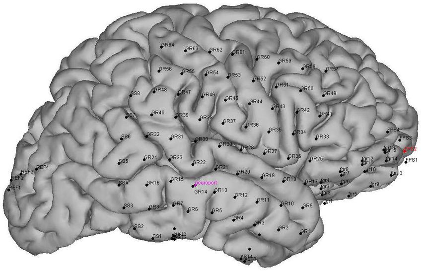
representative electrodes were chosen - one in the hippocampal region (Fig. 3A, left) and one close to the prefrontal part of the
cortex (Fig. 3A, right), which is known to receive direct hippocampal input (for details see Discussion) and is prone to initiate
Up-state [Nir et al., 2011, Sheroziya and Timofeev, 2014]. Recordings from the NREM phase of sleep were analyzed. SO were
detected in the frontal electrode (example shown in Fig. 3, top), while SWR were detected in the hippocampal electrode, see
example in Fig. 3B, bottom. We compared the locking between SWR and transition points of slow rhythm for both model and
experimental data. Several features were observed. First, there was increase of transitions from Up to Down state after SWR
(Fig. 3C, top), but not from Down to Up (Fig. 3C, bottom). Second, number of SWRs increased after transition to Up state
(Fig. 3D, bottom panels), but not after transition to Down state (top panels). The peak of SWRs in 3C, top corresponds to
peak of UDt in 3D, top. These empirical results were well captured by the model (compare Data and Model panels in each plot).
However, we observed more significant variations in number of events in the model vs recording data. This can be explained
by lower baseline activity in model simulations and it can be a results of much more synchronized activity between directly
connected cortical and hippocampal areas in the model.
Figure 3: A. Position of electrodes on the subject MG67. Left. Hippocampal depth electrodes image (RAT). Right. ECoG
electrodes positions on the same subject. B. Top. Raw LFP trace from ECoG, frontal pole electrode (FPS2, red circle at panel
A, right) showing alternating Up/Down states. Bottom. Raw LFP trace from depth electrode (in bipolar montage) from anterior
hippocampus (red circle on panel A, right) showing ripple following DUt at the top panel. The inset shows signal filtered at the
range of 80-120 Hz showing the ripple. Both panels are centered at the ripple (red vertical line, highest point in the analytical
amplitude envelope of the filtered signal). C&D. Comparison of model (20 independent trials, each simulating 50s of real time)
and experimental data (~16 h of NREM sleep). C. Ripple-triggered DUt/UDt histogram for the model and in the signal from
electrodes selected in the panel A. To get a smoother distribution, the transition event in each cell is measured separately in
the model; global transition in LFP is used for experimental data (see methods) D. DUt/UDt-triggered ripple histogram for the
model and in the signal. Global transition is used for both model and data. Red vertical line aligns with t = 0 ms.
4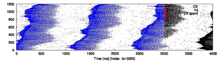
bioRxiv preprint first posted online Mar. 5, 2019; doi: http://dx.doi.org/10.1101/568881. The copyright holder for this preprint (which
            was not peer-reviewed) is the author/funder, who has granted bioRxiv a license to display the preprint in perpetuity.
                                           All rights reserved. No reuse allowed without permission.
Global coordination of SO-SWR rhythms is set by cortical drive
Next we set to investigate the mechanisms driving the relationships between cortical and hippocampal events reported in the
previous section. In Fig. 4A1 we again plot the DUt-triggered ripple-count histogram in which most of the ripples follow onset of
an Up-state. To find what determines this relationship, we considered two open-loop model configurations – one where only CX
targets HP and no connections are fed back from HP to CX (column B) and another one where only HP targets CX (column C).
As Fig. 4B1 shows, the network model with CX targeting HP preserves the phenomenon of DUt preceding the ripple event. In
contrast, in the model where HP targets CX but no feedback projections were implemented, no obvious coordination pattern was
observed (Fig. 4C1). We thus conclude that the global coordination of rhythms is set by the cortical drive to the HP network.
Still some differences to the closed loop model were observed. Removing HP->CX projections simplified the distribution that
only revealed one peak (compare Fig. 4 B1 and A1). Two sample Kolmogorov-Smirnov test comparing the distributions of
time-lags confirmed that the lags were derived from different distributions, p
bioRxiv preprint first posted online Mar. 5, 2019; doi: http://dx.doi.org/10.1101/568881. The copyright holder for this preprint (which
            was not peer-reviewed) is the author/funder, who has granted bioRxiv a license to display the preprint in perpetuity.
                                           All rights reserved. No reuse allowed without permission.
(red dots – high count of DUt events) can be explained by the fact that DUt transition increases the probability of the ripple
events and CA3 receives input from CX in this region (Fig. 1B, left). Therefore, ripples could likely be triggered by DUt events.
Consistent UDt activity (blue dots – high count of UDt events) in the same network region just follows the fact that Up-state
duration tends to be consistent across different cycles of SO. What makes Figs. 4 A3, B3 visibly distinct is the pattern of events
in the top region (high cell indexes). This pattern is very consistent in the closed-loop network (Fig. 4A3), where UDt (blue
dots) typically followed a ripple in the region receiving most of the CA1 input. This structure disappeared in the open-loop
network (Fig. 4B3) suggesting that hippocampal input to CX was able to synchronize the UDt events across neurons and across
many cycles of SO. In the following section we will discuss the mechanism that may lead to increased synchrony of UDt in the
closed loop network model.

Hippocampal influence on the slow oscillation

To better understand the impact of a ripple event on the dynamics of the cortical slow-wave we tested a simplified scenario.
The thalamocortical network was simulated in isolation with an input that was identical to a single hippocampal ripple (the
exact spiking of CA1 neurons was saved from simulation of the full TC-HP model) and that was applied at different times
corresponding to different phases of SO. Thus, for each trial, the cortical network was targeted only at one specific phase of slow
oscillation. We ran a set of such trials that uniformly spaced a full cycle of SO and we repeated this for many cycles of SO to
get average response. Fig. 5A shows an example of six trials when stimulation was applied at a different phase to the same cycle
of SO (so as to allow for a direct comparison between trials). Cortical spiking before (after) ripple injection is labeled in black
(blue); red spikes schematically interleaved in the region receiving HP input. Comprehensive animation of this experiment is
provided in SI Fig. 8. As we performed this experiment for many cycles of SO, several consistently repeating phenomena could
be observed. First, the ripple arriving at the very end of the Up-state was capable to increase its duration (compare Fig. 5 A5 vs
A1). Second, the ripple arriving approximately in the middle of the Down-state phase was capable of shortening that Down-state
and to cause DUt to start sooner (compare Fig. 5 A3 vs A1). Finally, the ripple arriving in the middle of the Up-state phase
was improving synchronization of DUt and mildly shorten it (compare Fig. 5 A6 vs A1). We confirmed these observations by
quantification across many different simulations of cortical dynamics (Fig. 5 B-D), including (1) an increase of Up-state duration
(the peak in Fig. 5B), (2) a decrease of Down-state duration (the dip in Fig. 5C) and (3) a decrease of standard deviation for
UDt times across neurons in the region receiving the ripple input (the dip in Fig. 5D).
The dip in the midst of a Down-state (Fig. 5C) suggests that ripples arriving during middle or later phase of a Down-state
(note that Down-state duration curve is skewed to the right) can increase probability of the network transition to an Up state.
This effect was not visible in the full closed-loop network analysis (Figs. 3,4), likely because of a sharp increase in the ripple
probability during Up-states has a hiding effect of a small number of ripples that occurred during Down-states (in other words
since most of the ripples occurred during the Up-state, statistically a single ripple was much more likely to be followed by a
Down-state than an Up-state; note however a small peak in DUt probability ~200 msec after ripple in Fig. 3C).
The dip in the midst of Up-state and the peak around UDt in Fig. 5D correspond to the dip/peak in Fig. 5B and another way
how they can be interpreted is that ripple occurring during an Up-state generally promotes synchronous transition to the Down
state except when precisely targeted at the very end of a Down state when it can extend its duration (see animations in SI Fig.
8). Increase in synchrony of UDt across cortical neurons during this simplified open-loop experiment suggests the possible cause
of the network synchronization observed in the close-loop model – i.e. highlighted blue region in Fig. 4 A3 showing synchronized
UDt in the area of network receiving ripple input (~#600-1000) following a ripple triggered in the late part of Up-state.
The last observation from simplified model was, furthermore, confirmed by running the following experiment. In complete
closed-loop TC-HP simulation we varied the delay from CA1 to CX pyramidal cell, thus effectively changing the phase of SO at
which cortex tends to receive a ripple. As a result, we observed that the pronounced (synchronized) structure of UDt in the top
region of the network (blue dots in Fig. 4A3) appeared mainly for short synaptic delays between CA1 to cortical pyramidal cells
(see SI Fig. 4 second/third column, row 1) but disappeared for longer delays (SI Fig. 9 second/third column, e.g., row 3). It is
worth noting that UDt-triggered ripple-count histogram in the scenario of shorter delays reveals a peak of ripples ahead of UDt
(see Fig. 4A2) suggesting “ripple as a cause of the Down-state”. However, at least in the case of our model, it was mainly the
synchronization of transition times to the Down state across population of cortical cell rather than transition to the Down-state
itself (which would occur nevertheless just with higher dispersion) which created the sharper peak in the ripple distribution.
The observation that ripples arriving in the midst of a Down-state shortened its duration (“triggered DUt”) from the simplified
model (Fig. 5) was also found in the closed-loop model (SI Fig. 4). When CA1->CX axonal delay became (unrealistically) long
so that most of the ripples tended to arrive at the midst of the Down-state following the Up-state (which helped to initiate the
sharp-wave events), we observed a highly synchronized region of DUt (SI Fig. 4, first column, e.g., 4th row, red dots) initiated
by the ripple event occurring in the late phase of the Down-state.

                                                                               6
bioRxiv preprint first posted online Mar. 5, 2019; doi: http://dx.doi.org/10.1101/568881. The copyright holder for this preprint (which
            was not peer-reviewed) is the author/funder, who has granted bioRxiv a license to display the preprint in perpetuity.
                                           All rights reserved. No reuse allowed without permission.

Figure 5: Ripple effect within a single SO oscillatory cycle, open loop scenario. A. A trace of a single representative ripple
event was saved from the closed loop simulation and delivered to the isolated thalamocortical network at the different phases
of the SO oscillatory cycle. Red dots show spikes of CA1 cells projected to the region of the cortical network. Blue dots are
spikes of cortical cells in the network without ripple stimulation, black dots are cortical spikes after the ripple was delivered.
The effect of a ripple on the spatiotemporal pattern of DUt/UDt transitions depended on the exact timing of the event. We
tested 100 independent trials with identical networks (each trial started with the same initial values of all variables) with the
ripple delivered at different times: Ti = i ∗ 20 ms for i-th trial. Each trial was repeated 10 times using different initial seed
values hereby creating different cortical dynamics; the results were averaged. Animation showing the described experiment is
shown in SI Fig. 8. To focus on the effect of a ripple, duration/synchronization effects and SO oscillatory cycle were defined by
cortical activity in the region receiving most of the ripple input (top 601-1200 cortical cells). B. Effect of ripple on the Up-state
duration. Top. Schematic diagram of cortical activity showing two Up-states (shaded) and single Down-state. Duration of the
first Up-state (blue envelope lines) was measured for each trial (different stimulation phase). Bottom. Average effect on Up-state
length from 10 runs. X-axis - timing of ripple rescaled to SO cycle (reference cycle for each trial was defined by the run where no
ripple was delivered). C. Effect of ripple on the Down-state duration. Top. Schematic diagram of of cortical activity. Duration
of the Down-state (blue-line envelope) was measured. Bottom. Average effect on the Down-state duration from 10 runs. D.
Effect of ripple on the synchrony of the UDt events. Top: Schematic diagram of cortical activity. Timing of the UDt events
(blue-line envelope) across population of cortical neurons was measured. Bottom: Average effect of ripple on the synchronization
of Up-state termination measured as a standard deviation of UDt events timing in the cortical neurons.

Ripples influence initiation probability
We found that ripple events targeting cortical neurons during specific phase of slow oscillation are capable of influencing the
structure and duration of Up and Down-states. To better understand the cumulative effect of the ripples targeting a specific
region of the cortical network, we considered two versions of synaptic wiring different by the connectivity pattern between the
hippocampus and cortex (Fig. 6 A1, B1). This included the original wiring (Fig. 6A1) in which a majority of the hippocampus-
triggered ripple output targets the region of cortex distant from the cortical region projecting to CA3 (and thus influencing
sharp-wave generation) – mirror mapping - and its plain version, in which ripple-active CA1 region projects to roughly the
same region which targets CA3 (Fig. 6 B1) – direct mapping. Simulations of both models revealed that the region receiving
most of the ripple input tended to become (after sufficient time; 50s of simulated time in total) a global initiator of the cortical

                                                                               7
bioRxiv preprint first posted online Mar. 5, 2019; doi: http://dx.doi.org/10.1101/568881. The copyright holder for this preprint (which
            was not peer-reviewed) is the author/funder, who has granted bioRxiv a license to display the preprint in perpetuity.
                                           All rights reserved. No reuse allowed without permission.
Up-states. Figures 6 A2/B2 show histogram profiles of the global Up-state initiation (two sample Kolmogorov-Smirnov test
comparing the distributions of global initiators confirmed that they were derived from different distributions, pcortical connections (X-axis) decreases. The mean spatial profile of the DUt is displayed as a heatmap on
Fig. 6 A3/B3 where for each DUt “wave” a zero time lag indicates global ignition site (i.e. the first cortical cell which pass
through DUt transition in a given SO cycle). Since in the mirror (direct) mapping model Up-states are more likely to start
in the top (bottom) region of the cortex, this defines a preferred direction of the traveling DUt wave. This observation was
further confirmed by measuring an average gradient of the traveling wave for each local neighborhood of neurons that revealed
an opposite traveling wave direction for the two network topologies (Fig. 6 A3/B3, histograms). This phenomenon was robust
with respect to the phase of SO being hit by the ripple, see SI Fig. 9, 4th column, since varying the time delay of CA1->CX
projections did not change the overall shape of DUt traveling wave.
    Preferential direction of the DUt activity propagation could have an impact on the synaptic strength if we consider the spike-
time dependent plasticity (STDP) form of learning. Indeed, the cortical network model used in our study reveals spindle-like
activity in the beginning of each Up-state which was generated by the thalamic component of the model [Bazhenov et al., 2000,
Wei et al., 2018], see zoom-in of the spike waves in Fig. 2 bottom left. Spindles provide suitable time window for the STDP rule
to be effective [Muller et al., 2016]. In our network model, each cortical pyramidal neuron was connected symmetrically to both
sides of its close neighborhood. Thus, for each preferred direction of wave traveling, this would lead to synaptic connections
decreasing strength in one direction and increasing it in the opposite direction. We estimated synaptic changes by calculating
STDP offline from spike traces recorded in the simulation. Figure 6 A4/B4 shows changes to synaptic weights in close vicinity
(X-axis) of each pyramidal neuron (Y-axis) for mirror (left) and direct (right) connectivity models. In the mirror model (Fig.
6A4), synapses from neurons with higher index to the neurons with lower index (corresponding to the traveling wave direction)
were generally increased and opposite synapses decreased. When comparing Fig. 6 A4 and B4 we found that two wiring scenarios
tend to produce symmetrically opposite synaptic changes as consequence of opposite direction of the traveling wave.

                                                                               8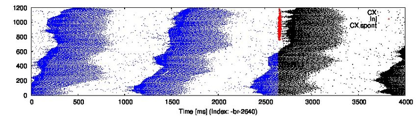
bioRxiv preprint first posted online Mar. 5, 2019; doi: http://dx.doi.org/10.1101/568881. The copyright holder for this preprint (which
was not peer-reviewed) is the author/funder, who has granted bioRxiv a license to display the preprint in perpetuity.
All rights reserved. No reuse allowed without permission.
A1 B1
A2 B2
1200 1200
1000 1000
Cortical neuron
800
Cortical neuron 800
600 1200
P(Initiation) x 10−3
2 600
1.8
1000
1.6
Cortical neuron
1.4
800
400 1.2
400
600 1
0.8
400
0.6
0.4
200 200
0.2
200
0
125% 100% 75% 50% 25% 0%
Connectivity strength
0 0
0 0.5 1 1.5 2 2.5 0 0.5 1 1.5 2 2.5
Global initiation x 10
−3 Global initiation x 10
−3
A3 B3
1200 1200
1000 1000
1050 1050
Cortical neuron
Cortical neuron
800 800
750 750
600 600
400
450 400
450
200 150 200 150
0 500 1000 −0.5 0 0.5 0 500 1000 −0.5 0 0.5
Lag to global initiation [ms] Gradient Lag to global initiation [ms] Gradient
A4
1200
B4
1200
0.1 0.1
1000 1000
Cortical neuron
Cortical neuron
0.05 0.05
800 800
600 0 600 0
400 400
−0.05 −0.05
200 200
−0.1 −0.1
−15 −11 −7 −3 0 3 7 11 15 −15 −11 −7 −3 0 3 7 11 15
Distance to neighbouring neuron Distance to neighbouring neuron
Figure 6: Hippocampal ripples shape slow wave spatiotemporal pattern. A1, B1. Two wiring models (A1, mirror) and (B1,
direct) reveal different spatiotemporal patterns of cortical slow waves. A2, B2. Probability of global initiation for each neuron in
the network. In A1 ripples target the ‘top’ region of the cortex (cells [601-1200]) and cause higher Up-state initiation likelihood
in that region (A2, blue). In B1 ripples target the ’bottom’ region ([1-600]) and cause higher initiation in that region (B2, blue).
Averages across 20 trials, dotted lines show standard error of the mean. A2 inset: Impact of ripples depends on the strength
of CA1->CX connections. Color map codes probability of global Up state initiation for each neuron in a A1 wiring scenario.
The preference for the upper region initiation dissolves as CA1->CX connectivity strength decreases (100% corresponds to the
A2 case, 0% corresponds to cortical dynamics without CA1 input). A3,B3. The change of the Up-state initiation probability is
reflected in the shape of the DUt traveling wave. A3/B3, left. Probability of DUt for each neuron as a function of time (lag)
with respect to the time moment of a global DUt (zero lag). A3/B3 right. Difference of the gradient (“slope” in radians) of the
DUt traveling wave in the mirror and direct map models compared to the cortex-only model (cortex receives no hippocampal
input), each bar corresponds to restricted region of 100 neurons. Positive values indicate a higher tendency of waves to propagate
from the bottom to the top of network when compared to the cortex-only model, while the negative values show the opposite
tendency. A4,B4. Change of “incoming” synapses strength (X-axis - relative index of a presynaptic neuron in respect to the
index of a fixed postsynaptic neuron) calculated using offline STDP. The neurons in the middle of the network show an opposite
trend for strengthening/weakening of synapses, corresponding to preferred slope gradients as shown A3/B3. The effect starts
weakening around the distance of 10 neighboring neurons (X-axis) which is due to the increasing time delay.
9
bioRxiv preprint first posted online Mar. 5, 2019; doi: http://dx.doi.org/10.1101/568881. The copyright holder for this preprint (which
            was not peer-reviewed) is the author/funder, who has granted bioRxiv a license to display the preprint in perpetuity.
                                           All rights reserved. No reuse allowed without permission.
Discussion
Hippocampo-cortical dialogue is critical for consolidation of memory [Preston and Eichenbaum, 2013]. Coordination between
the prominent oscillations during sleep – cortical slow oscillations and hippocampal ripples – was proposed to be the primary
orchestrating mechanism in this dialogue [Buzsáki, 1996, Maingret et al., 2016]. In this new study, we investigated the reciprocal
influence of two major sleep rhythms in the large-scale model implementing slow oscillations in the thalamo-cortical network
[Bazhenov et al., 2002, Wei et al., 2018] and SWRs in the CA3-CA1 hippocampal network [Malerba et al., 2016, Malerba and
Bazhenov, 2018]. Out study revealed a complex pattern of interaction between the rhythms where hippocampal ripples were able
to bias cortical network to initiate Down to Up state transitions at specific cortical network locations as well as to synchronize
Up to Down state transitions. This prediction may explain the mechanism behind the role of hippocampal ripples in defining
cortical spike sequences replay during sleep related memory consolidation [Inostroza and Born, 2013].
    Many specific details of the functional connectivity between (m)PFC and hippocampus are not fully known. Anatomically, the
existence of connections from hippocampus to PFC is well established - CA1/subiculum connections to PFC were independently
described in mice [Parent et al., 2009], rhesus monkey [Goldman-Rakic et al., 1984, Barbas and Blatt, 1995, Averbeck and
Seo, 2008], cat [Irle and Markowitsch, 1982, Cavada et al., 1983] and in greater detail in rats (for review see Cenquizca and
Swanson [2007]), where CA1 makes monosynaptic connections to (m)PFC to both excitatory and inhibitory cells [Gabbott et al.,
2002] with latency in the order of 15-20 ms [Ferino et al., 1987, Laroche et al., 1990, Dégenètais et al., 2003, Tierney et al.,
2004]. In line with anatomical findings, recordings during the sleep found that CA1-mPFC unit interactions were distributed
widely but not uniformly across the cells and showed about 10 ms latency between CA1 and mPFC followers [Wierzynski et al.,
2009]. Furthermore, there is a converging evidence that hippocampo-cortical pathway is plastic and activated during memory
consolidation [Laroche et al., 2000].
    Projections from PFC (anterior cingulate, ACC) back to CA1 were found in mice [Rajasethupathy et al., 2015] but parallel
recording of ACC and CA1 units during SWS suggested a rather multisynaptic pathway [Wang and Ikemoto, 2016]. Weak
projection between (o)PFC and CA1 was also described in rhesus monkey [Carmichael and Price, 1995] but it’s existence
remains questionable [Cavada et al., 2000]. Thus, communication from PFC to hippocampus is likely to be mediated through
the main input gate – entorhinal cortex [Lavenex and Amaral, 2000, Preston and Eichenbaum, 2013].
    In agreement with these empirical studies, in our model the CA1 region projected widely into the ‘prefrontal’ cortex network,
but the connectivity was not uniform, instead CA1 was parceled into small regions which targeted specific focal points in the
cortical network (see diagram in Fig. 1B). In the opposite direction a small patch of the cortical network projected directly to
CA3. Thus, effectively during slow-wave sleep, cortical input to the hippocampus was activated only when a traveling wave of
Down to Up state transition [Massimini et al., 2004, Luczak et al., 2007, Murphy et al., 2009, Nir et al., 2011] reached that
cortical patch. Without explicit modeling of dentate gyrus/rhinal cortices we considered this simplified model as a functional
approximation of the intricate mechanism of how cortical input enters and affects hippocampus in vivo [Hahn et al., 2007].
    Other important pathways omitted in the model included the nucleus reuniens (NR) targeting both CA1 & mPFC [Hoover
and Vertes, 2012, Varela et al., 2014] and mPFC -> NR -> CA1 pathways [Vertes, 2006, Vertes et al., 2007] possibly gating
mPFC->hippocampal flow which was shown to be important for memory consolidation [Ito et al., 2015].
    Hippocampal SWRs were hypothesized to be a mediator of the hippocampo-cortical dialogue during deep sleep Buzsáki
[1996] and indeed experimental studies revealed that cortical cells may fire in coordination with hippocampal ripples [Siapas and
Wilson, 1998]. Unlike short SWR events (50-100 msec), cortical slow waves (0.2-1 Hz) are characterized by relatively smooth
transitions between Up and Down states, so direct comparison of the timing of the SWR and SO events across the published
studies is difficult. In many studies SWR preferably occurs during an Up-state [Mölle et al., 2006, Isomura et al., 2006, Nir
et al., 2011], but see also [Battaglia et al., 2004, Hahn et al., 2007]. Another common reference points of the SO are transitions
between Up and Down states; it was reported that SWRs commonly follow transition from Down to Up state in the cortical
network [Sirota et al., 2003, Battaglia et al., 2004, Isomura et al., 2006, Mölle et al., 2006]. There is also evidence that SWRs
precede cortical Down-state [Peyrache et al., 2009, Maingret et al., 2016, Peyrache et al., 2011].
    To study interaction between SO and SWRs ripples, we used the biophysical TC-hippocampal model and observed realistic
coupling behaviour between cortically generated slow oscillation and hippocampally generated ripples. In agreement with [Iso-
mura et al., 2006], we observed clear biasing of the SWR probability by DUt; UDt transition probability increased following the
ripple and causal effect of ripples was confirmed by cutting CA1->CX projections in open-loop experiment. While only a small
fraction of SWRs occurred in the model during cortical Down-states, these events could still bias network location of UP-state
initiation site. Open-loop (CA1->CX) simulations, where SWR was artificially triggered at different pre-defined phases of SO,
revealed that the effect of SWR fundamentally depends on the phase of SO, namely we observed that i) UDt events could be
both delayed or advanced by SWR; ii) synchronization of UDt events could be both improved or reduced; iii) DUt events could
be only advanced; and iv) in general Up-state initiation could not be directly triggered by a single SWR event unless it occurred
in very close proximity to DUt where local initiation could be observed. That is in line with experimental findings [Isomura
et al., 2006] where SWR event during the Down-state was sometimes capable to trigger spiking but the network returned back
to the Down state without transition to the Up-state. Similar observations led Buzsáki [2015] to suggest that in anesthesia SWR
do not routinely bias the phase of slow oscillations. Our simulations suggest that while no immediate Up-state typically follows
SWR events occurring during Down state, the duration of the ongoing Down state changes and thus the phase of SO may be
affected as well. The model prediction that the ripple, occurring in the mid-late phase of an Up-state, is capable of advancing
and synchronizing UDt, may explain data showing visible peak of ripple probability before Down-state in the UDt-triggered

                                                                              10
bioRxiv preprint first posted online Mar. 5, 2019; doi: http://dx.doi.org/10.1101/568881. The copyright holder for this preprint (which
was not peer-reviewed) is the author/funder, who has granted bioRxiv a license to display the preprint in perpetuity.
All rights reserved. No reuse allowed without permission.
ripple count histogram [Peyrache et al., 2011, Maingret et al., 2016] and may shed light on the mechanisms behind apparently
more synchronized UDt compared to DUt events in vivo [Volgushev et al., 2006, Chen et al., 2012]. The dependence of the
SWR effect on the SO phase reported here is also in line with the experimental work of [Batterink et al., 2016], showing the
existence of optimal time (with respect to SO phase) for the auditory input in targeted memory reactivation that improves
memory consolidation in sleep.
We omitted in our model analysis of spindles - a very important component of the SPW-SO interaction. Studies show
ripple-spindle locking [Sirota et al., 2003, Mölle et al., 2006, Clemens et al., 2007, Wierzynski et al., 2009]; a recent work reported
phase-locking between SWR, SO and spindles [Latchoumane et al., 2017] and their nesting within hippocampus [Staresina et al.,
2015]. While it is clear that spindle density is an important marker for memory consolidation processes [Mednick et al., 2013],
the exact functional role is not clear. A recent proposal suggests SO as the leader of active memory consolidation while spindle
functionally deafferenting cortical circuitry from SWR input [Genzel et al., 2014] thus helping (selective) reorganization during
Up-state following SWR reactivation-Down state complex [Maingret et al., 2016].
The question about temporal coordination of DUt/UDt and SWRs is directly related to the hypothesis of the cortical and
hippocampal spike sequence replay during sleep, which is believed to be necessary for stabilizing recent memory traces [Wilson
and McNaughton, 1994, Nakashiba et al., 2009, van de Ven et al., 2016, Valero et al., 2017]. Cortical replay occurs during
Up-state [Johnson et al., 2010], peaking close to the transition points [Isomura et al., 2006, Peyrache et al., 2011]. Hippocampal
replay occurs in CA1 during the ripple events [Kudrimoti et al., 1999], it is known to be concurrent with cortical replay and both
pre-cortical (PFC)[Peyrache et al., 2009] and post-cortical (visual cortex) [Ji and Wilson, 2007] coupling was observed, leading
to the discussion whether the CA1 sequences are driven by SO or SWR drives replay in PFC [Genzel et al., 2014, Buzsáki, 2015].
In [Rothschild et al., 2017] it was shown that there is a bilateral dialogue between the auditory cortex (AC-CX) and CA1, where
AC-CX pre-SWR firing predicted SWR content, which in turn predicted post-SWR AC-CX activity, thus suggesting a possible
scenario in which a single ripple is first triggered by the cortex and intermediately influences the cortex back within a single
oscillation cycle.
In this study, we did not attempt to model sequence replay. We observed, however, that repeated ripple events targeting
a specific cortical region can reshape spatiotemporal patterns of Up-state initiation. This leads to consistent change in how
Up-state waves travel across the cortical network. SWS firing patterns were found to be supportive for induction of long-term
synaptic plastic changes [Chauvette et al., 2012], so we tried to assess how spike-time dependent plasticity [Bi and Poo, 2001]
during slow-waves would shape the synaptic connectivity on the cortical site. We found that spatial location/distance to the
cortical cells which are targets of the ripple determined whether STDP would render the synapses weakened or strengthened,
thus allowing the mechanism which selects the ripple content to influence plasticity on the cortical site. Different hippocampal
assemblies representing distinct sequences participating in the ripple event(s) could project into various cortical targets leading
to parallel reorganization at different cortical sites. Observed reorganization by SWR is consistent with experimental results of
[Maingret et al., 2016] in which proper timing of SWR (with respect to cortical Down-state) is able to reorganize mPFC firing
patterns, which would otherwise stay stable [Luczak et al., 2007].
Methods
Hippocampal module
The model is tuned to show appropriate stochasticity in the spontaneous occurrence of sharp-wave ripples and large irregular
activity in the interleaning times. The firing rates of excitatory and inhibitory cells in the system are consistent with experimental
in vivo data, and the CA3-CA1 model activity in isolation from cortical input was studied in terms of the ripple mechanism
[Malerba et al., 2016], the synaptic connections role on reactivation during ripples [Malerba and Bazhenov, 2018] and the
relation between reactivation during sleep and synaptic changes induced by awake learning [Malerba et al., 2017b]. Technically,
the model closely follows that of [Malerba et al., 2016, Malerba and Bazhenov, 2018] with a slight difference in CA3 connectivity
and projections to CA1, which leads to a single main excitable region in CA3 generating all the sharp waves, rather than
stochastically evolving locations in CA3 which were observed otherwise. Here we briefly describe the basic properties of the
model. CA1 model consists of 800 excitatory and 160 interneurons, CA3 has 1200 excitatory cells and 240 interneurons. Each
neurons is described by the following equations
v − Vt
C v̇ = −gL (V − EL ) + gL ∆ exp − w + I(t)
∆
τw ẇ = a(v − EL ) − w
v(t) = Vthr ⇒ v(t + dt) = Vr , w(t + dt) = w(t) + b
I(t) = IDC + Isyn (t) + gN Iη
where v is membrane potential and w slow variable. For CA1 pyramidal cells C = 200 pF, gL = 7 nS, EL = −58 mV,
∆ = 2 mV, Vt = −50 mV, τw = 120 ms, a = 2, Vthr = 0 mV, Vr = −46 mV, b = 100 pA; for CA3 pyramidal cells b = 40 pA; for
both CA1/CA3 inhibitory neurons these parameter change: gL = 10 nS, EL = −70 mV, b = 10 pA, Vr = −58 mV, τw = 30 ms.
11bioRxiv preprint first posted online Mar. 5, 2019; doi: http://dx.doi.org/10.1101/568881. The copyright holder for this preprint (which
was not peer-reviewed) is the author/funder, who has granted bioRxiv a license to display the preprint in perpetuity.
All rights reserved. No reuse allowed without permission.
IDC input is a constant different for each cell selected from Gaussian distribution, mean µ (in pA) and standard deviation p %
expressed as a percent of the mean value was different for each population of pyramidal (µCA1 = 40, pCA1 = 10%, µCA3 = 22.5,
pCA3 = 30%) and inhibitory (µCA1 = 180, pCA1 = 10%, µCA3 = 130, pCA3 = 30%) cells.
We construct the background noise by generating two incoming surrogate spike trains (one excitatory and one inhibitory)
and convolving each spike train with an exponential decay, and finally combining the two into a current signal Iη . The two
spike trains are built as memoryless, by finding the time of the next surrogate spike using an exponential random variable (note
that exponential inter-arrival times are markings of memoryless Poisson Processes). To numerically obtain the exponential inter-
arrival times of the surrogate spikes, we used a well known conversion from uniform random variables to random variables of a
given distribution (inverse transform sampling). Practically, the next time a surrogate spike was generated as R = t − log(S)/λ,
where λ = 0.5 ms−1 was the rate of incoming spikes, t was the current simulation time, and S a uniformly sampled random
variable. Hence, we had two surrogate spike trains (with the same high rate), we convolved each of them with a exponential
decay time (τD = 1 ms), shaping two noisy signals with a small standard deviation. Finally, we subtracted the inhibitory signal
from the excitatory signal, and scaled the resulting signal (noisy, with one pole decay after the λ rate, and with small standard
deviation) by a constant coefficient which was tuned to induce, when the current was added to a mildly hyperpolarized single
cell, a standard deviation in voltage fluctuations of about 2 mV. Technically, this was obtained by scaling the noise added to
excitatory cells by gN = 110.08, and to inhibitory cells by gN = 92.88.
The synaptic current from excitatory (SAM P A ) and inhibitory(SGABA ) synapses to neuron n was defined as:
X X
g j→n sj→n (t) ∗ (vn − EGABA ) + g j→n sj→n (t) ∗ (vn − EAM P A )
Isyn (t) = −
j∈SGABA j∈SGABA
t−tk
t−tk
H H
X
sj→n = F e τd
−e τd
tk
where reversal potentials were EGABA = −80 mV and EAM P A = 0 mV, tk are the spikes times from the presynaptic cell j.
F is a normalization coefficient, set so that every spike in the double exponential within parentheses peaks at one, and H is
the Heaviside function, ensuring that the effect of each presynaptic spike affects the post-synaptic current only after the spike
AM P A AM P A AM P A
has happened. Decay and rise constants were τr (P y −→ P y) = 0.5, τd (P y −→ P y) = 3.5, τr (P y −→ In) = 0.9,
AM P A GABA GABA GABA GABA
τd (P y −→ In) = 3.0, τr (In −→ P y) = 0.3, τd (In −→ P y) = 3.5, τr (In −→ In) = 0.3, τd (In −→ In) = 2.0; CA3
AM P A AM P A
P y → In synapses had distinct constants τr (P yCA3 −→ InCA3 ) = 0.5, τd (P yCA3 −→ InCA3 ) = 3.0.
Synaptic weights were sampled from Gaussian distributions with variance σ given by percent of the mean µ: N AM P A (µ =
P yCA3 −→ P yCA3
22, σ = 0.3µ), N AM P A (µ = 50, σ = 0.3µ), N GABA (µ = 35, σ = 0.3µ), N GABA (µ = 40, σ = 0.3µ),
P yCA3 −→ InCA3 InCA3 −→ InCA3 InCA3 −→ P yCA3
N AM P A (µ = 66, σ = 0.04µ), N AM P A (µ = 275, σ = 0.04µ).
P yCA3 −→ P yCA1 P yCA3 −→ InCA1
The rationale for the choice of the equations and parameters is in length discussed in [Malerba et al., 2016, 2017a, Malerba
and Bazhenov, 2018].
Thalamo-cortical module
Our TC-CX module is similar to previous models Bazhenov et al. [2002], Krishnan et al. [2016], Wei et al. [2018] aimed at
modeling stage 3 sleep. Neuromodulatory changes for different sleep stages and STDP plasticity at synapses were not employed
in this model.
All neurons follow Hodgkin-Huxley kinetics, cortical neurons included dendritic and axo-somatic compartments:
dVd
Cm = −IdK−leak − Idleak − IdN a − IdN ap − IdKm − IdKCa − IdCa − I syn
dt
gcs (Vd − Vs ) = −IsN a − IsK − IsN ap
2
where the subscripts s and d correspond to axo-somatic and dendritic compartments. Cm = 0.75 µF/cm , I K−leak is
the potassium leak current, Idleak Cl− leak currents, IdN a fast Na+ currents, IdN ap persistent sodium current, I K fast delayed
rectifier K+ current, I Km slow voltage-dependent non-inactivating K+ current, I KCa slow Ca2+ dependent K+ current, I Ca
high-threshold Ca2+ current, and I syn is the sum of all synaptic currents to the neuron. The intrinsic currents had generally
the form I current = g current (V − E current ). Details of individual currents can be found in the previous publications [Bazhenov
2
et al., 2002, Chen et al., 2012, Wei et al., 2016]. The conductances of the leak currents were g K−leak = 0.004 mS/cm and
2 2
g leak = 0.012 mS/cm . The maximal conductances for the voltage and ion-gated intrinsic currents were gdN ap = 2.1 mS/cm ,
Na 2 Ca 2 KCa 2 Km 2 Na 2 K 2
gd = 0.8 mS/cm , gd = 0.012 mS/cm , gd = 0.05 mS/cm , gd = 0.02 mS/cm , gs = 3000 mS/cm , gs = 200 mS/cm ,
2
gsN ap = 15 mS/cm . For inhibitory neurons persistent sodium current was not present (I N ap = 0) and conductances of the
2 2
leak currents were: g K−leak = 0.003 mS/cm and g leak = 0.01 mS/cm . The maximal conductances for the voltage and
2 2 2 2
ion-gated intrinsic currents were gdN a = 0.8 mS/cm , gdCa = 0.012 mS/cm , gdKCa = 0.05 mS/cm , gdKm = 0.015 mS/cm ,
Na 2 K 2
gs = 2500 mS/cm , gs = 200 mS/cm .
12bioRxiv preprint first posted online Mar. 5, 2019; doi: http://dx.doi.org/10.1101/568881. The copyright holder for this preprint (which
was not peer-reviewed) is the author/funder, who has granted bioRxiv a license to display the preprint in perpetuity.
All rights reserved. No reuse allowed without permission.
Thalamic neurons were single-compartmental neurons following the equation:
dV
= IdK−leak − I leak − I N a − I K − I h − I LCa − I syn
dt
where I N a and I K are fast Na+ /K+ currents, and I h hyperpolarization-activated depolarizing current. For TC neurons leak
2 2
currents conductances were g K−leak = 0.035 mS/cm , g leak = 0.01 mS/cm , and maximal conductances for other currents were
2 2 2 2
g N a = 90 mS/cm , g K = 12 mS/cm , g LCa = 2.5 mS/cm , g h = 0.016 mS/cm . For RE neurons I h current was not present
h K−leak 2 leak 2 2 2
(I = 0), and conductances were g = 0.006 mS/cm , g = 0.05 mS/cm , g N a = 100 mS/cm , g K = 10 mS/cm ,
LCa 2
g = 2.2 mS/cm .
The synaptic currents for AMPA, NMDA, GABAA , GABAB synapses were described by first order activation schemes in the
form of Isyn = gsyn [O]f (V )(V − Esyn ) where gsyn is maximum conductance, [O] is the fraction of open channels, Esyn is the
reversal potential, the details for each synaptic current is described in [Wei et al., 2016].
AM P A N M DA AM P A
The maximal conductances were g(P y −→ P y) = 0.076 µS, g(P y −→ P y) = 0.003 µS, g(P y −→ In) = 0.096 µS,
N M DA GABAA AM P A GABAA
g(P y −→ In) = 0.008 µS, g(In −→ P y) = 0.3 µS, g(T C −→ RE) = 0.032 µS, g(RE −→ T C) = 0.015 µS,
GABAB GABAA AM P A AM P A
g(RE −→ T C) = 0.001 µS, g(RE −→ RE) = 0.07 µS, g(T C −→ P y) = 0.04 µS, g(T C −→ IN ) = 0.114 µS,
AM P A AM P A
g(P y −→ T C) = 0.001 µS, g(P y −→ RE) = 0.005 µS.
The synapses between hippocampus and cortex were modeled as AMPA synapses from above with the possibility of sig-
AM P A AM P A
nal transmission delay maximum conductances g(P yCA1 −→ P yCX ) = 0.006 µS, g(P yCX −→ P yCA3 ) = 0.142 µS,
AM P A
g(P yCX −→ InCA3 ) = 0.067 µS, their connectivity will be described in the next section. The default synaptic delay were
16 ms [Ferino et al., 1987] for CA1->CX and 30 ms for CX->CA3 (functionally mimicking several synaptic hops needed for the
cortical layer 5 signal reaching CA3 in hippocampus) connections, the small delay of CA1->CX connections did not have strong
effect on the results and we set it to 0 ms later in order to have equal sampling distance when the effect of synaptic delays was
explored (see Fig. 9).
Additionally in PY->PY, PYIN cortical connections miniature EPSP/IPSP [Redman, 1990, Salin and Prince, 1996] were
present, their arrival times were modeled by Poisson processes with time-dependent mean rate µAM P A (t) = (2/(1 + exp(−(t −
AM P A
t0 )/τ )) − 1)/250 and µGABAB (t) = log((t − t0 + 50)/50)/400 with t0 is a time of last presynaptic spike, τ (P y −→ P y) = 20,
AM P A AM P A AM P A
τ (P y −→ In) = 40. The maximal conductances for minis were g(P y −→ P y) = 0.106 mS, g(P y −→ In) = 0.016 mS,
GABA
g(In −→ A P y) = 0.242 mS.
Network connectivity
The global topology between the different modules can be seen in Fig. 1A., the connectivity between different neuronal types can
be seen in Fig. 1B. Network connectivity of thalamocortical module is similar to the previous studies [Wei et al., 2018]. Cortex
(CX) consisted of 1200 layer-5 pyramidal neurons (Py) and 240 inhibitory neurons (In), thalamus consisted of 240 TC and 240
RE cells. Each neuronal type had local one-dimensional single-layer connectivity determined by the radii of connections (Fig.
AM P A N M DA AM P A
1D,E). The radii of cortical and thalamic connections were r(P y −→ P y) = 10, r(P y −→ P y) = 10, r(P y −→ In) = 2,
N M DA GABAA AM P A GABAA GABAB
r(P y −→ In) = 1, r(In −→ P y) = 10, r(T C −→ RE) = 6, r(RE −→ T C) = 6, r(RE −→ T C) = 6,
GABA AM P A AM P A AM P A AM P A
r(RE −→ A RE) = 5, r(T C −→ P y) = 50, r(T C −→ IN ) = 10, r(P y −→ T C) = 25, r(P y −→ RE) = 20. Network
connectivity of hippocampal module is similar to [Malerba and Bazhenov, 2018], see Fig. 1C.
CA3 consisted of 1200 excitatory cells and 240 interneurons and had one-dimensional topology. The probability of connection
from CA3 pyramidal cell with index i to other CA3 pyramids and interneurons was proportional to p = 1 − (1 − 0.15) ∗ (i/1200),
i.e. the subnetwork with smaller index numbers was more densely connected to increase the probability of SWR initiated in
this region. The probability of connection from CA3 interneurons to CA3 pyramids was uniform, p = 0.7. The connectivity
of Schaffer collaterals from CA3 pyramids with index i to CA1 pyramids and interneurons was inversely proportional, i.e.
p = 1 − (1 − 0.15) ∗ ((1 − i)/1200), so that more interconnected CA3 regions projects less to CA1 and vice versa. Within CA1
connectivity was all-to-all (including both Py and In), but synapses which were sampled at zero or less weight were removed
from the connectivity, yielding to approximately 50% of CA1 Py-Py connections being cut (details in the next section).
In order to couple only the subdivision of the cortical network with hippocampus, only continuous subset of cortical pyramidal
AM P A AM P A
cells with index i ∈ [200; 399] project to subset of CA3 neurons with radii r(P yCX −→ P yCA3 ) = 10, r(P yCX −→ InCA3 ) =
1. For the opposite direction flow from hippocampus to cortex, continuous chunks of 100 CA1 pyramidal neurons were targeting
small continuous chunks of 5 cortical pyramids. CA1 chunks were partially overlapping (each subsequential chunk being shifted
by 20 neurons), cortical chunks were non-overlapping with the gap of 33 neurons. Within the single CA1-CX chunk pair every
CA1 neuron projected to all neurons of cortical chunk. The pairing between the chunks was linear and flipped, so that CA1
chunks with small index targeted chunks with high CX index and vice versa. Although by connectivity CA1 region targeted
distinct loci of the whole cortical network, effectively most of the ripple input (see the histogram of firing across CA1 cells in
Fig. 2, left top) was received by cortical sites opposite to the subregion projecting to CA3 thanks to the flip. Although far from
real anatomical connectivity, this topology was chosen in order to be compatible with the following properties: 1. CA1 projects
13You can also read