The population dynamics of a canonical cognitive circuit - bioRxiv
←
→
Page content transcription
If your browser does not render page correctly, please read the page content below
bioRxiv preprint first posted online Jan. 9, 2019; doi: http://dx.doi.org/10.1101/516021. The copyright holder for this preprint (which
       was not peer-reviewed) is the author/funder, who has granted bioRxiv a license to display the preprint in perpetuity.
                                       All rights reserved. No reuse allowed without permission.

      The population dynamics of a canonical cognitive circuit
       Rishidev Chaudhuri1 , Berk Gerçek1,2,* , Biraj Pandey1,* , Adrien Peyrache3 ,
                                   and Ila Fiete1,4,†
             1
              Center for Learning and Memory and Department of Neuroscience,
                         The University of Texas, Austin, Texas, USA.
                               2
                                 Department of Basic Neuroscience,
                          University of Geneva, Geneva, Switzerland.
            3
               Department of Neurology and Neurosurgery, Montreal Neurological
                                            Institute,
                         McGill University, Montreal, Quebec, Canada.
            4
              Current address: Department of Brain and Cognitive Sciences, MIT,
                                 Cambridge, Massachusetts, USA.
                       *
                         B.G. and B.P. contributed equally to this work.
                            †
                              Correspondence: fiete@mit.edu (I.R.F.)

                                                       Abstract
                  The brain constructs distributed representations of key low-dimensional variables.
              These variables may be external stimuli or internal constructs of quantities relevant
              for survival, such as a sense of one’s location in the world. We consider that the high-
              dimensional population-level activity vectors are the fundamental representational cur-
              rency of a neural circuit, and these vectors trace out a low-dimensional manifold whose
              dimension and topology matches those of the represented variable. This manifold
              perspective — applied to the mammalian head direction circuit across rich waking be-
              haviors and sleep — enables powerful inferences about circuit representation and mech-
              anism, including: Direct visualization and blind discovery that the network represents
              a one-dimensional circular variable across waking and REM sleep; fully unsupervised
              decoding of the coded variable; stability and attractor dynamics in the representation;
              the discovery of new dynamical trajectories during sleep; the limiting role of external
              rather than internal noise in the fidelity of memory states; and the conclusion that the
              circuit is set up to integrate velocity inputs according to classical continuous attractor
              models.

           It has long been clear that the brain represents sensory, motor, and internal variables in

                                                                         1
bioRxiv preprint first posted online Jan. 9, 2019; doi: http://dx.doi.org/10.1101/516021. The copyright holder for this preprint (which
       was not peer-reviewed) is the author/funder, who has granted bioRxiv a license to display the preprint in perpetuity.
                                       All rights reserved. No reuse allowed without permission.

      distributed codes across large populations of neurons. In turn, theoretical models of com-
      putation in the brain have emphasized that neural circuit dynamics must be understood in
      terms of the emergence of simple structures from the collective interactions of large num-
      bers of neurons 1–8 , and that robust representation and memory involve the formation of
      low-dimensional attractors in the population dynamics.
          Until relatively recently, experimental techniques permitted access to only one or a few
      neurons at a time, but simultaneous recordings of multiple neurons are making feasible
      the theoretically suggested approach of characterizing the structure and dynamics of neural
      responses at the population level. This approach is beautifully illustrated in recent demon-
      strations of low-dimensional trajectories in sensory and motor circuits 9–12 .
          Our work proceeds from four central premises: 1) In distributed codes, information rep-
      resentation, computation, and dynamics unfold at the level of the neural population and
      the collective states of a circuit are the natural way to understand them. 2) If a circuit
      represents a low-dimensional variable of given dimension and topology, the high-dimensional
      states of the circuit will be localized to a low-dimensional subspace or manifold of matching
      dimension and topology. 3) Characterizing the structure of this manifold can enable un-
      supervised discovery and decoding of the internally coded (latent) variable. 4) Examining
      manifold structure and dynamics on and o↵ the manifold across a range of behavioral states
      as the inputs to the circuit change can reveal aspects of circuit mechanism.
          We illustrate a method to characterize the manifold structure of data, use this character-
      ization to discover, in a blind or unsupervised way, low-dimensional internal states, provide
      a blind time-resolved decoding of these states, and provide support for the predictions of a
      classic mechanistic circuit model, using the mammalian head direction system as our sub-
      ject. The head direction (HD) system in mammals and insects 13–21 is a high-level cognitive
      circuit that uses various external and internal cues to compute an estimate of the direction
      of heading of the animal with respect to the external world. It is a proving-ground for the
      manifold-based approach to unsupervised discovery of the encoded variables because it rep-
      resents internal cognitive states that need not directly reflect externally measured variables
      during waking, and this dissociation between internal and external states holds even more
      true during sleep (as we will see). At the same time, the HD system also helps us illustrate
      how a manifold approach can yield genuinely new insight into the structure, dynamics, and
      mechanisms of a long-studied neural circuit.
          Two decades ago, theoretical models 4;22–25 of the HD circuit predicted the existence of a
      stable, one-dimensional (henceforth 1D) ring-shaped stable manifold in the high-dimensional
      state space of the population activity, a more abstract and fundamental feature than details
      about the shapes of tuning curves, connectivity profiles, or physical placements of neurons
      in the circuit. The notion of stability means that perturbations of any kind in the high-
      dimensional space away from the ring should quickly and preferentially flow back to the
      ring. If the HD circuit is an integrator, then the states along the ring and changes in state
      along the ring for equivalent changes in the represented variable should in some sense be
      equal. The basic elements of the HD circuit models have since been extended to explain
      the dynamics of other neurons, including grid cells 7 . The same circuit models can further
      explain how, through the integration of a di↵erent velocity signal, the brain could form
      representations in more abstract metric spaces 26;27 . Thus, testing the extent to which these
      models are really correct descriptors of circuit mechanism is a question of broad importance.

                                                                         2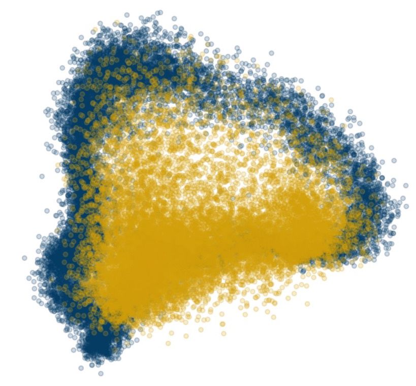
bioRxiv preprint first posted online Jan. 9, 2019; doi: http://dx.doi.org/10.1101/516021. The copyright holder for this preprint (which
       was not peer-reviewed) is the author/funder, who has granted bioRxiv a license to display the preprint in perpetuity.
                                       All rights reserved. No reuse allowed without permission.

          So far, pairwise correlations between mammalian HD cells 15;28–32 and a topographically
      ordered physical HD-coding ring structure in flies 18–21 are consistent with the hypothesized
      models. Here we show directly that the long-hypothesized low-dimensional state-space ring
      structure and attractive dynamics can be directly visualized in the population responses of
      the mammalian HD system. The dynamics revealed in this circuit during sleep states provide
      new evidence about the mechanisms that allow these states to be maintained and updated.
          Portions of these results have been presented at conferences 33;34 .

      Results
      The instantaneous (temporally binned) response of N neurons is a point in an N -dimensional
      state space where each axis represents the activity of one neuron (Fig. 1a). The collection
      of such snapshots of the population activity forms a cloud in the state space. If the popula-
      tion encodes some variable of dimension Dm ⌧ N and a certain topology, the point cloud
      should trace out a manifold of the same dimension and topology, although the shape may
      be convoluted. In what follows, we describe how characterizing the manifold’s topology and
      structure, then analyzing dynamics on the manifold, can permit us to extract the latent
      encoded variables in an unsupervised way and deduce key aspects of circuit mechanism.

      Spline parameterization for unsupervised decoding (SPUD)
      We characterize the global topology of the manifold using methods of topological data analy-
      sis, specifically persistent homology 35 : The method starts from the point-cloud of data, Fig.
      1a, blurring the points at di↵erent resolutions or scales, and at each resolution examining the
      emergence of connected groups of data points called simplicial complexes, Fig. 1b. A sim-
      plicial complex can contain certain structures within it, such as a ring or a torus and so on.
      Betti numbers form a list of binary structural designations that characterize the complexes:
      A complex that is (topologically) equivalent to a flat, holeless sheet of some dimension has
      only a non-zero Betti-0 number; all higher-order Betti numbers are zero. A (convoluted)
      ring or a cylinder, each of which enclose a single hole, have a non-zero Betti-0 number and
      Betti-1 number, but none of higher-orders; a figure-8 shaped complex will have a non-zero
      Betti-0 number and two Betti-1 numbers, but none of higher order; a (hollow) torus, which
      contains two circular holes and one two-dimensional void, has a non-zero Betti-0 number,
      two Betti-1 numbers and one Betti-2 number; and so on for more complex objects. In noisy
      data, if a Betti number for a structure persists over many scales (Fig. 1b), this feature is
      robust against noise and thus deemed significant. Topological data analysis prescribes how
      to characterize the Betti numbers of complexes in a dataset 35 .
           To decode the internal state encoded by the manifold, we perform the following steps
      (details in Methods): 1) Consider the binned spiking data as points in a high-dimensional
      state space, Fig. 1a; 2) Determine the topology of the point cloud using methods of topolog-
      ical data analysis (TDA), specifically persistent homology 35 , Fig. 1b, and the introduction
      of a neighborhood-thresholded TDA (nt-TDA) for increased robustness to noisy data (see
      SI S2.2); 3) estimate intrinsic local manifold dimension using various methods including cor-
      relation dimension 36 , Fig. 1c; 4) Fit the manifold with a spline of matching topology and

                                                                         3
bioRxiv preprint first posted online Jan. 9, 2019; doi: http://dx.doi.org/10.1101/516021. The copyright holder for this preprint (which
       was not peer-reviewed) is the author/funder, who has granted bioRxiv a license to display the preprint in perpetuity.
                                       All rights reserved. No reuse allowed without permission.

       a   data manifold in state space          b manifold topology: persistent homology                     c local dimension: several methods
                                                                                            Betti-1 barcode

                                                                                                                               log(pts in ball)
                                                                                              2 3 4 5 6
                                                                                              simpl radius

                                                                                               radius of
                                                                                               simplicial                                         23456
                                                                                               complex                                            ball radius

      d fit spline of matched topology, dim e       parametrize spline by latent variable                     f   unsupervised decoding

      Figure 1: Population activity as a manifold and a method for manifold characterization.
      (a) Each blue point is a vector representing instantaneous activity in the neural population: vector
      component (ri ) is the activity of the ith neuron. The points form a manifold. (b) Persistent
      homology to determine topology for general manifolds: Balls of di↵erent size centered on the
      datapoints represent di↵erent simplicial radii (r) or scales. At a given radius, sets of connected
      points form simplicial complices (SI S2 for details). Each complex is characterized by a set of
      Betti numbers; depicted here are the loop features of the complices (colored rings), at the di↵erent
      scales. Loops appear in panel 2 and disappear (are filled in) by panel 3; another appears in panel
      3 and persists until the last; it is deemed significant because of its persistence. Inset: Betti-1
      barcode, or the range of radii over which each loop persists. (c) Local dimension can be estimated
      by several methods. Schematic shows correlation dimension: Count the number of points in a ball
      of radius r centered at a point on the manifold, as a function of r. The number of points should
      grow as rDm if the manifold is Dm dimensional. (d) The data manifold is fit by a spline (cyan
      line) of dimension and topology as determined in (a-c). The spline uses a few anchor points (cyan
      circles) determined by clustering methods, with connecting polynomial curves. (e) The spline is
      parametrized by assigning coordinates along its length. The coordinates represent the values of
      an internal (latent) state that the circuit is assumed to encode. (f) Moment-by-moment decoding
      of the internal state is done by reading out the parametrization value at the point on the spline
      closest to the datapoint.

                                                                         4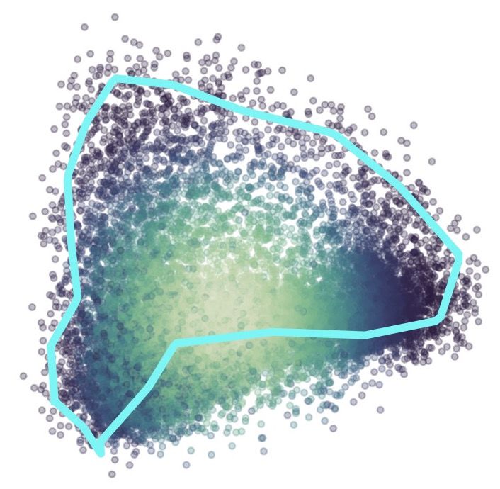
bioRxiv preprint first posted online Jan. 9, 2019; doi: http://dx.doi.org/10.1101/516021. The copyright holder for this preprint (which
       was not peer-reviewed) is the author/funder, who has granted bioRxiv a license to display the preprint in perpetuity.
                                       All rights reserved. No reuse allowed without permission.

      dimension, Fig. 1d; 5) Parametrize the spline by a smoothly changing variable of match-
      ing dimension and topology, Fig. 1e; the resulting parametrization is interpreted as the
      values of the encoded latent variable or internal state. 6) Given a population state at any
      moment in time, decode that state by projecting it to the nearest point on the spline; the
      parametrization value at that point is the unsupervised estimate of the value of the encoded
      latent variable, Fig. 1f. In this entire decoding process, when the manifold is topologi-
      cally non-trivial in structure, constructing a low-dimensional embedding is neither necessary
      (though nonlinearly embedding the manifold into some intermediate-dimensional space can
      be practically useful for efficient spline fitting, for modestly improving the spline fits because
      the embedded manifold has fewer narrow kinks or convolutions (SI Fig. S4 to see the modest
      gains from dimensionality reduction when one is data-limited), and for visualization when
      the manifold dimension is sufficiently small), nor is it sufficient. Dimensionality reduction
      provides a global coordinate system that is not sufficient for obtaining a minimal parameter-
      ization for manifolds that are not topologically equivalent to some hole-free K-dimensional
      sheet: For instance, the minimum embedding dimension for a 1D ring is 2D, and dimen-
      sionality reduction will yield at best a global 2D parametrization of the 1D variable, which
      represents a failure to discover the real 1D latent variable. This problem is general for all
      topologically non-trivial manifolds, because there is an important di↵erence between global
      and local coordinates, and global coordinates provide either a non-unique or too-high di-
      mensional parametrization of the manifold. The on-manifold parameterization method we
      describe yields a local rather than global coordinate system to describe the manifold, and
      extracts the correct one-dimensional structure of the encoded variable.

      Ring manifold and unsupervised decoding in the mammalian HD
      system
      We apply SPUD to neural activity data recorded from the anterodorsal thalamic nucleus
      (ADn) of mice that are awake and foraging in an open environment along random, variable
      paths with variable velocities, as well as during intervening REM and nREM periods 32 . Note
      that the animal’s waking behavior is not low-dimensional: Unlike in many other applications
      of manifold methods 10;12 , the animal is not constrained to move along specific trajectories
      or perform a stereotyped task. Further, during sleep the neural dynamics are not known to
      be externally constrained in any way.
         We show manifolds and compute Betti barcodes for the best session in each of the 7
      recorded animals (Figs. S1, S7 and S11). All remaining results are based on the (3/7)
      animals where the RMS di↵erence between measured and decoded angle during waking is
      < 0.5 rad. For any session that we use for unsupervised decoding, we include all recorded
      thalamic cells, with no sub-selection based on tuning. For each cell, instantaneous firing
      rates are obtained by convolution with a Gaussian kernel (100ms standard deviation).
         The first problem is to determine whether the data exhibit some simple low-dimensional
      manifold structure in state space. The states of the network during waking exploration
      appear — through direct visualization of a nonlinear low-dimensional embedding from the
      high-dimensional state space 37a – to lie on a strikingly low-dimensional albeit highly non-
          a
              The manifold is sufficiently convoluted that it does not occupy a very low-dimensional linear subspace,

                                                                         5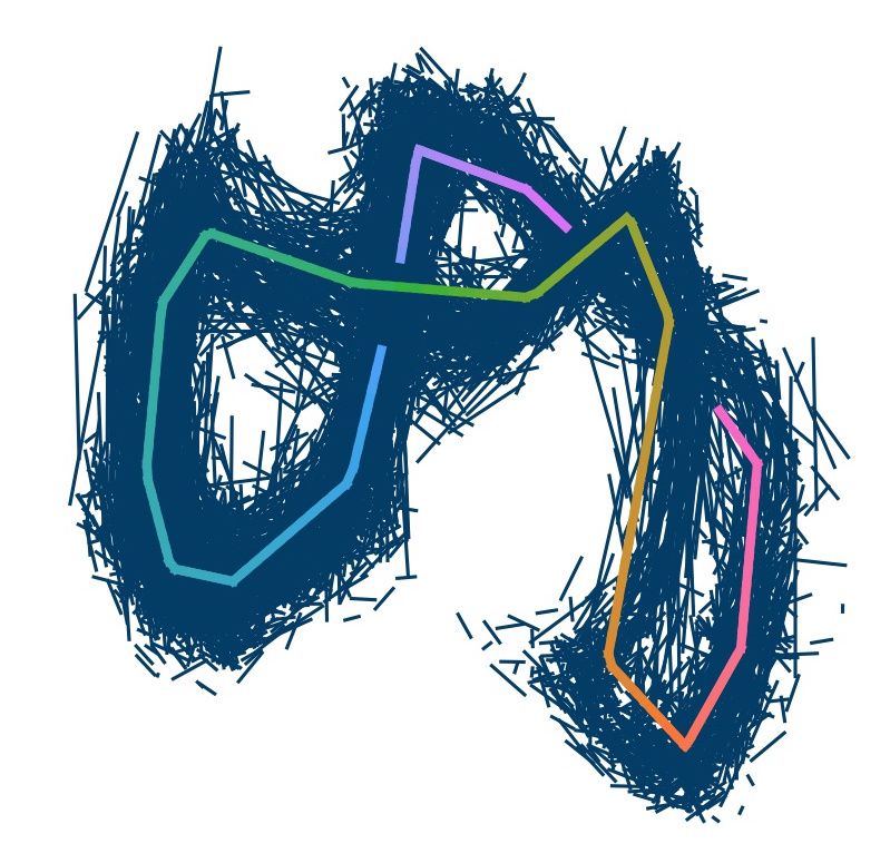
bioRxiv preprint first posted online Jan. 9, 2019; doi: http://dx.doi.org/10.1101/516021. The copyright holder for this preprint (which
was not peer-reviewed) is the author/funder, who has granted bioRxiv a license to display the preprint in perpetuity.
All rights reserved. No reuse allowed without permission.
a b c d e
H0
H1
H2
0 radius (√ Hz) 45
f SPUD
g i 1 *** * *** * 1
meas SPUD
meas
angle (rad)
-
frac var
frac var
-
0 0 0
200 time (s) 400 Mouse 12 Mouse 25 Mouse 28 Mouse 12 Mouse 25 Mouse 28
h j k Cij (raw) Cij\ meas Cij\ SPUD
160 100 25 10 5 1 22
firing rate (Hz)
neuron
0.5
prob
0 0 0 0 0 0 1
1 neuron 22
0 2 2
0.0 0 Hz 100 Hz
angle ( , ) 0 dist (√ Hz) 10
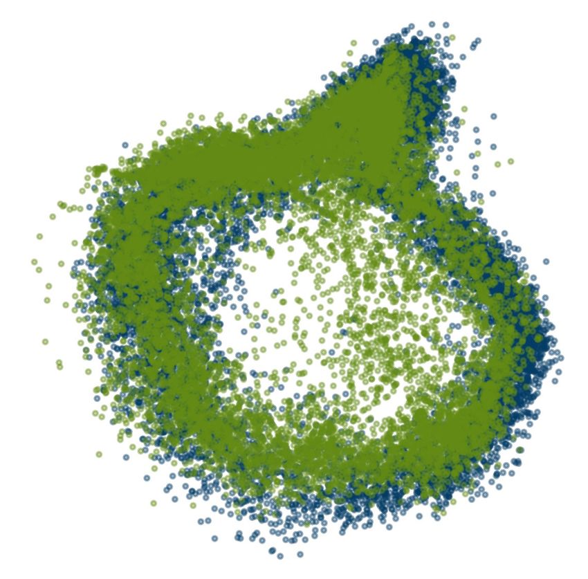
Figure 2: Unsupervised discovery and time-resolved decoding of encoded variable
through manifold characterization. Throughout, ✓ = direct measurement of the animal’s
head orientation from LED tracking; ✓ˆ = supervised decoder’s estimate of the brain’s represen-
tation (using tuning curves); ↵ = unsupervised latent variable estimate. This figure: ADn data
from single animal for full waking episode (31 minute interval). (a) Visualization of manifold (by
Isomap 37 ), with every alternate pair of temporally adjacent points connected. Inset shows point
cloud (top) and alternate view of manifold (bottom). Note that PCA often fails to pull out the
ring structure of manifold, Fig. S2. (b) Betti-0, -1 and -2 barcodes: Simplicial complex radii on
abscissa (schematic at top: complexes constructed from data at di↵erent radii): the start and end
of a horizontal bar in the middle plot signals the appearance and disappearance of some ring (a
non-zero
p Betti-1 feature) in the data
p at the corresponding radii. Long bar: a ring that appears at
⇠ 16 Hz and persists until ⇠ 43 Hz (for description of analysis and units see S2). (c) Spline fit to
point cloud. (d) Parametrization of spline by coordinate ↵ (arbitrary origin). (e) Coloring of neural
states by unsupervised latent variable estimate (i.e., ↵). (f) Comparison of ↵ and ✓. (The origin
and direction around the ring for measured head angle and for unsupervised decoding, both arbi-
trary choices, are matched to facilitate comparison, only after unsupervised decoding is complete.)
(g) Histogram of di↵erences between ↵ and ✓ and between ↵ and ✓. ˆ (h) Fully unsupervised tuning
curve estimate (blue) versus supervised tuning curve estimate (black). (i) Left: Average fraction
of variance explained by ✓ (black) and ↵ (blue) under a Poisson spiking model (solid bars) and an
overdispersed (hatched bars) model. Error bars show standard error; significance is from two-sided
binomial test (see SI S5). Right: Variance explained for individual cells under Poisson model, with
means shown in orange. (j) Manifold from data (blue) and from an overdispersed spiking model
(red), with overdispersion estimated from the data (see SI S5) and applied as uncorrelated across
neurons. Inset shows distribution of distances from manifold fit for data and model. (k) Covariance
of firing rates (left) and covariance conditioned on either ✓ or ↵.
6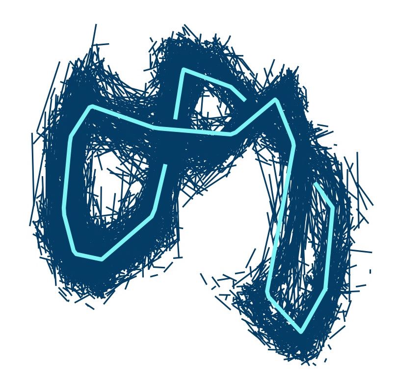
bioRxiv preprint first posted online Jan. 9, 2019; doi: http://dx.doi.org/10.1101/516021. The copyright holder for this preprint (which
       was not peer-reviewed) is the author/funder, who has granted bioRxiv a license to display the preprint in perpetuity.
                                       All rights reserved. No reuse allowed without permission.

      linear manifold, in the form of a convoluted ring, Fig. 2a (see Fig. S1 for all 7 animals in
      the data set, and Supplementary Movie 1 for a 3D view). Because waking behavior is not
      low-dimensional, the low-dimensional structure we see is intrinsic, rather than imposed by
      the environment or task.
          To independently verify that the structure visualized in the embeddings is real rather
      than an artefact of the visualization process, and that important, higher-dimensional and
      topological structures are not lost, we turn to topological data analysis, in particular the per-
      sistent homology of simplicial complexes 35 . Topological methods are more general because
      they permit characterization of manifolds that are topologically non-trivial in structure and
      higher-dimensional 35 , when direct visualization is not possible.
          From the persistent homology of simplicial complexes constructed from the waking data
      (see Methods), we confirm an open loop or ring structure in the data that persists over
      several spatial scales (H1 plot, Fig. 2b), and also find no evidence of a toroidal or more
      complex topological structure (H2 plot, Fig. 2b; contrast Figure S3). As shown below, there
      is no evidence of additional structure down to the resolution of the data.
          With the confirmation of a ring topology, we fit to the manifold a nonlinear spline with
      the same topology (Fig. 2c) and then isometrically parameterize the spline along its length
      with a circular variable whose values are indicated by the color of the spline (Fig. 2d). Points
      on the manifold are colored according to the nearest parameterization value (Fig. 2e).
          Strikingly, the decoded latent variable very closely matches (up to an arbitrary choice
      of origin and direction) the directly measured head angle (from LED’s on the animal’s
      head), Fig. 2f,g (see Fig. S4 for other animals). The match serves as a direct validation
      that the extracted ring structure is real, and of the hypothesis that the topology of neural
      representations should match the topology of the represented variables.
          It was not clear a priori that an isometric parameterization would suffice for this level of
      accuracy in decoding. The fact that isometric parameterization along the neural population
      response manifold produces excellent decoding implies that equal amounts of neural code
      length or activity variation are given to equal changes in head angle and that therefore
      no specific angles are favored for greater representational resources than others, exactly
      consistent with the expectations for an head velocity integrator circuit, in which all states
      have to be equivalently represented and equivalently changeable so that a unit velocity input
      produces a unit change in represented angle regardless of the angle. This isometry property
      enables accurate integration of a velocity signal regardless of starting angle.
          Next, we regress the time-varying firing rates of individual cells onto the latent variable
      estimate. This allows us to recover neural tuning curves in a fully blind way, Fig. 2h.
      The unsupervised tuning curves capture 71% ± 2.8% of the variance of tuning curves con-
      structed the traditional, supervised way (Fig. S5). Relatively flat tuning curves are also
      consistent across the supervised and unsupervised estimates under the assumption of an en-
      coded variable that is one-dimensional and circular; cells with flatter curves are slightly but
      not significantly more overdispersed in their spiking relative to well-tuned cells (correlation
      between variance of tuning curve and overdispersion is 0.25, p of 0.12; data not shown).
          The unsupervised latent variable estimate appears to more faithfully track the internal
      thus linear embedding methods are of limited use and can create artefactual self-intersections in the manifold
      projection. Nonlinear embedding methods 37–39 are less prone to these problems.

                                                                         7
bioRxiv preprint first posted online Jan. 9, 2019; doi: http://dx.doi.org/10.1101/516021. The copyright holder for this preprint (which
       was not peer-reviewed) is the author/funder, who has granted bioRxiv a license to display the preprint in perpetuity.
                                       All rights reserved. No reuse allowed without permission.

      representation of head angle than it does the measured HD, assessed from the even closer
      match between the latent variable estimate and internal state estimate constructed from
      a supervised (tuning-curve-based) decoder of HD circuit activity (Fig. 2g; Fig. S4, S5
      for other animals). Indeed, the measured HD is not guaranteed to accurately report the
      animal’s internal representation, which may slip relative to the measured HD for various
      reasons, including the possibility that the animal is uncertain about its HD, is representing
      past or future HD states, or because of errors in the experimental measurement of HD.
      Further, our latent variable estimate explains more of the variance of neural spiking (cross-
      validated, Fig. 2i) than does the measured HD, a confirmation that the unsupervised latent
      variable estimate is a more accurate reflection of the internal representation of HD (see Fig.
      S5 for further controls including leave-one-cell-out analyses where the variance of a neuron
      is explained using SPUD and activity in the rest of the population).
           A natural question is whether the waking manifold encodes additional variables not yet
      discovered, for example in the thickness of the ring. With a finite signal-to-noise ratio (SNR)
      in the dataset it is impossible, with any method, to exclude the possibility of structure in
      the data that is significantly smaller than the noise. However, we may search for additional
      coding structure down to the resolution limit imposed by noise, by asking whether the data
      exhibits a spread or structure not explained by the 1D ring structure together with inde-
      pendent neural spiking noise. We thus generate synthetic data based only on the 1D latent
      variable extracted through SPUD, with spikes generated independently (after conditioning
      on the 1D variable) using an independent point process per cell with dispersion matched
      empirically to the data. The structure and spread of the resulting point cloud closely match
      those in the real data, Fig. 2j, suggesting that the circuit is not encoding additional vari-
      ables in the form of shared (correlated) structure in other dimensions of its response. (By
      contrast, we do find an additional coding dimension in postsubicular HD cells (coding for
      head velocity; data not shown) as well as in ADn during nREM sleep (shown later)).
           We search further for small-scale cooperative coding beyond the 1D ring in the popula-
      tion response by directly examining patterns of covariation between neurons after removing
      the e↵ects of their shared angular coding around the ring manifold, Fig. 2k. Patterns of
      correlation are strong before conditioning on the angular variable, but weak after (the ratio
      of the Frobenius norm of the residual covariance matrix to the norm of the raw covariance
      matrix is only 6% when conditioning on the unsupervised latent variable estimate, suggesting
      that it captures ⇠ 94% of the data covariance; by contrast, the ratio after conditioning on
      measured HD is 25%, consistent with earlier findings that measured HD is a worse indicator
      of internal state than our unsupervised estimate). These results demonstrate that there is
      little discernible additional structure in the waking manifold, and the ADn appears to sup-
      port the encoding of only a single one-dimensional circular variable during waking, down to
      the resolution (SNR) of the present data.
           The SNR in these data and results is primarily limited by the number of simultaneously
      recorded cells. Larger samples of simultaneously recorded neurons will improve SNR and
      reduce the scatter around the ring, allowing discovery of finer additional structure or further
      downgrading the possibility that it exists.

                                                                         8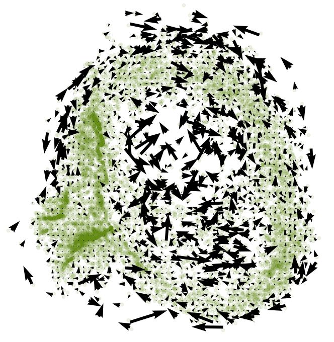
bioRxiv preprint first posted online Jan. 9, 2019; doi: http://dx.doi.org/10.1101/516021. The copyright holder for this preprint (which
       was not peer-reviewed) is the author/funder, who has granted bioRxiv a license to display the preprint in perpetuity.
                                       All rights reserved. No reuse allowed without permission.

      The ring manifold is autonomously generated and attractive
      Above, we highlighted how regarding neural population responses as lying on a manifold and
      then characterizing the structure of the manifold can permit unsupervised decoding of latent
      variables. In what follows, we show how the manifold view reveals the collective dynamics of
      the circuit, in a direct, easy, and natural way. First, we will consider coarse-grained net flows
      of states on and o↵ the manifold. Second, we will consider the fine time-resolved dynamics
      of trajectories on the manifold.
          Through these analyses, we test the key predictions 1;3;4;7 of continuous attractor network
      models (properties 1-4) and models of neural integrators for continuous variables (properties
      1-5), Fig. 3a (see Fig. S6 for a network model): 1) The high-dimensional network response
      occupies a low-dimensional continuum of states with dimension and topology matching those
      of the encoded variable(s). 2) The states are autonomously generated and stabilized, and
      capable of self-sustained activation when sensory inputs are removed. 3) The manifold is
      an attractor: states initialized away from the manifold flow rapidly back toward it. 4)
      The states along the manifold are energetically equal, with no flux or net flow along the
      manifold. 5) A velocity input, encoding the time-derivative of the represented variable,
      drives the circuit in a special direction, specifically, along the low-dimensional manifold in
      the high-dimensional state space. Note that these predictions are fundamentally in terms of
      the population manifold, hence most naturally tested at that level, when the data make it
      possible.
          Results above already directly support property 1). To study autonomous dynamics, we
      examine the states of the circuit during sleep, when the circuit no longer receives spatial or
      directional input from the world. During REM sleep, the states again lie on a ring, Fig. 3b
      (and Supplementary Movie 2), and moreover are essentially identical to those from awake
      exploration, laying on the same ring manifold, Fig. 3c (Fig. S7 for other animals). The
      result is in direct support of property 2), and consistent with a similar previous conclusion
      inferred from preserved pairwise correlations during sleep 32 .

      States on the manifold are energetically flat or equivalent
      To test the equivalence of states along the manifold, we examine the coarse occupancy and
      dynamics of manifold states during REM sleep, when the circuit is not driven by the external
      world (spatial exploration could be biased). First, we construct instantaneous (undirected)
      vectors or bars linking states at adjacent time-points, Fig. 3d; the length of a bar is pro-
      portional to the mean speed at that time. If the manifold contained a few prominent sinks
      or discrete fixed points, there would be fast flow to and high occupancy around those fixed
      points, which would correspond visually to long bars converging near those points. As one
      can see, the lengths and density of the bars are roughly uniform across both waking and
      sleep manifolds in a given session, Fig. 3d.
          Separately but related, the change in angle is independent of the value of the angle itself,
      Fig. 3e (Fig. S8 for other animals). To obtain a quantifiable measure of occupancy along
      the ring and to gain statistical power from pooling across sessions and days from a single
      animal, we decode the angular states on the ring with a supervised decoder, and compute
      the density of decoded angles, Fig. 3f. The logarithm of the density of states along the ring

                                                                         9
bioRxiv preprint first posted online Jan. 9, 2019; doi: http://dx.doi.org/10.1101/516021. The copyright holder for this preprint (which
       was not peer-reviewed) is the author/funder, who has granted bioRxiv a license to display the preprint in perpetuity.
                                       All rights reserved. No reuse allowed without permission.

       a                                                                    b                                 c

                                                                                H0
                                          E
                  1                             4
                          2

                                                                                H1
                              3
                      5

                                                    5

                                                                                H2
                                                                                 0        radius (√ Hz)   8

       d                                                e       1                                  g                      h
                                                            ↵

                                                             -1
                                                                                     ↵
                                                        f -1.5
                                                                                                                           i
                                                            log(P( ))

                                                                                                                               1.8        ***

                                                                                                                               voff/von
                                                             -4                                                                0.5
                                                                        0

      Figure 3: REM sleep states, fluxes, and dynamics suggest that the manifold is internally
      generated and attractive. (a) Schematic of attractor model predictions (see main text for list).
      (b) Betti-1 barcode reveals 1D ring structure preserved during REM sleep. (c) Joint visualization
      of REM (green) and waking data (dark blue) using Isomap 37 . (d) Flows along REM manifold:
      each bar represents a velocity vector at a moment in time. Inset shows wake manifold. (e) Single
      session mean and standard deviation of change in decoded angle as a function of angle. (f) Mean
      and standard deviation of angle occupancy (from tuning curve decoder) across sessions. (g) Flux
      on and o↵ manifold. (h) Schematic showing that flux should be small on manifold, because velocity
      vectors tend to point in both directions along manifold and thus average out (top panel), while
      flux o↵ manifold should be large, because velocity vectors tend to point towards manifold (bottom
      panel). (i) Ratio of size of flux vector o↵ manifold to flux vector on manifold. Error bars show
      standard deviation; hatched bar shows shu✏ed control (p < 10 6 ; see SI S8).

                                                                                     10
bioRxiv preprint first posted online Jan. 9, 2019; doi: http://dx.doi.org/10.1101/516021. The copyright holder for this preprint (which
was not peer-reviewed) is the author/funder, who has granted bioRxiv a license to display the preprint in perpetuity.
All rights reserved. No reuse allowed without permission.
– a direct estimate of the relative energy of these states – is flat on the scale of the variability
across sessions. These results directly support property 4).
Finally, we examine the fluxes or net flows of states on versus o↵ the manifold. The
flux through a small region is the vector average over all the instantaneous trajectories that
flow into and out of that region, Fig. 3g. For a continuous attractor not being driven by
a directed input, we expect at most small net flows or fluxes along the manifold because of
the uniform distribution of flows in all directions along the manifold (property 4), as well
as because of the omnidirectional and unbiased nature of random kicks o↵ the manifold;
however, we expect large net fluxes for states that are not on the manifold because of biased
flows of states returning to the manifold (property 3), precisely as seen in the data, where
the fluxes are small on-manifold, but large for points o↵-manifold (Fig. 3g-i).
Di↵usive dynamics along manifold during REM
After obtaining a detailed qualitative picture of states and dynamics on and near the mani-
fold, we combine theoretical predictions about dynamical trajectories on continuous attractor
manifolds 40 with our ability to perform time-resolved unsupervised decoding using SPUD
(Fig. 4a-b) to gain a quantitative estimate of the nature and influence of noise on the circuit.
Noise is an important consideration for integrator, memory, and representational circuits,
because it determines the timescale and fidelity of information stored in the circuit.
First, we validate that SPUD can sufficiently capture the fine-time-scale statistics of
trajectories based on the available data by comparing time-lagged correlations of the unsu-
pervised latent variable estimate during waking and against a “ground truth” of measured
HD correlations, Fig.4c (blue and black traces in inset). Since HD updates during waking are
correlated in time (Fig. 4d, blue trace and Supplementary Movie 3), the squared deflection
in angle over time grows quadratically at short times (Fig. 4c, left inset).
During REM sleep, by contrast, angular updates are temporally uncorrelated but never-
theless local (SPUD result in Fig. 4d, green trace, and Supplementary Movie 4; the angle
change histogram is small and unimodal), and the squared angular deflection grows linearly
with time (Fig. 4c green curve). These two features — uncorrelated local updates together
with a linear growth in squared deflection over time — are characteristic of an unbiased
di↵usive random walk, consistent with property 4) if the dynamics during sleep are noise-
dominated and if the noise lacks temporally coherent structure 40 .
Evidence of input aligned to manifold
To resolve the nature of the noise driving di↵usivity during REM, we make, to our knowledge,
the first quantitative comparison between empirically-observed di↵usion in a neural circuit
and theoretical predictions. The di↵usion constant of REM dynamics in Fig. 4c is 1.1 ± 0.04
rad2 /s (0.52 ± 0.03 and 1.3 ± 0.06 for the other two animals; see Fig. S9). This di↵usivity
exceeds, by a factor of 20-50, the predicted value in a matched model (see 40 , SI S10 and Fig.
S10), Fig. 4c, if the noise in the circuit is independent across neurons.
Independent per-neuron noise could arise from Poisson spike count variations within the
circuit, or from a high-dimensional input that projects in a spatially uncorrelated way to
the neurons. In either case, such high-dimensional noise is impotent in pushing the network
11bioRxiv preprint first posted online Jan. 9, 2019; doi: http://dx.doi.org/10.1101/516021. The copyright holder for this preprint (which
was not peer-reviewed) is the author/funder, who has granted bioRxiv a license to display the preprint in perpetuity.
All rights reserved. No reuse allowed without permission.
state along the manifold, because noise of unit variance only has a projection of size 1/N
along the manifold 4;40;41 , Fig. 4e. Increasing the amplitude of independent noise is not a
solution: even 5x overdispersed noise does not account for the di↵erence in di↵usion constant,
and independent noise of large magnitude destroys the low-dimensional states of the circuit
(other factors that might potentially contribute to the gap between predicted versus observed
di↵usivity fall far short of accounting for the discrepancy, SI S10).
By contrast, a modest amount of noise in the form of fluctuations aligned to the nonlinear
manifold, which is naturally interpreted as arriving in the velocity input to the circuit, has
a much stronger e↵ect 40;41 . Noise on the same order of magnitude as the velocity strengths
required to produce HD-matched changes in represented angle in a model (standard deviation
of 8.5 rad/s1/2 , with temporal correlations of 20 ms or less; compare waking in Fig. S4),
is sufficient to account for the measured di↵usion, Fig. 4c. Noise aligned to the manifold
additionally tends not to distort the activity states, and thus more purely moves the states
along the manifold with at most small o↵-manifold e↵ects, as apparently seen in the REM
data. In sum, with high probability, REM di↵usivity is driven by a low-dimensional noise
injected into the circuit through an input aligned to the manifold, and thus likely arriving
through the velocity pathway, with a magnitude consistent with the size of waking velocity
inputs into the circuit (property 5).
These results demonstrate that even in high-level cognitive circuits for memory and in-
tegration, as previously established for low-level sensory circuits and sensorimotor path-
ways 42–45 , input noise or sensory precision rather than internal noise is the limiting factor
for information fidelity.
Inputs during nREM sleep disrupt ring manifold
Hippocampal circuits replay patterns of waking activity during nREM sleep 46–49 , and these
events may play an important role in memory consolidation 50 . However, the HD circuit seems
to lack replays or even coherent temporal dynamics 32;51 . On a more abstract level, nREM
sleep is thought to disrupt the brain’s ability to maintain integrated representations 52 , but
it is unclear what this means at a more granular level, for specific integrated representations
like HD. A manifold-based approach reveals when previous population-level structure is
modified and helps to understand the nature of the modification. In addition, if there is
coherent dynamics in the restructured space, a manifold-based approach can help find it,
even if the structure is not visible when states are projected into the old space.
The manifold in nREM does not preserve the ring structure of waking and REM states: it
is higher-dimensional (persistent homology, contrast Fig. 4f with Fig. 2b, 3b; visualization,
Fig. 4g and Supplementary Movie 5; also see correlation dimension estimates in Fig. S11),
and only partially overlaps the waking/REM manifold (Fig. 4g).
The higher-dimensional nREM manifold encodes at least two latent variables. We decode
an angle along the tangential (circular) dimension of the manifold using SPUD, and compare
it with the outputs of two wake-trained supervised decoders that make di↵erent assumptions:
a tuning-curve decoder and a population vector decoder (Fig. S12). The angles decoded by
all three methods agree well (see Fig. S13 for another animal), except at low-activity states
where the signal-to-noise ratio of the neural response is low.
A second latent variable obtained from the radial dimension of the manifold (based on
12bioRxiv preprint first posted online Jan. 9, 2019; doi: http://dx.doi.org/10.1101/516021. The copyright holder for this preprint (which
was not peer-reviewed) is the author/funder, who has granted bioRxiv a license to display the preprint in perpetuity.
All rights reserved. No reuse allowed without permission.
a h250
(Hz)
rate
1s
0 Low High
time (s)
b i
0 25
c d j k1
diff const (rad2/s)
0.2 1 2.25
acorr( )
coherent
1 wake
REM
acorr( )
0.6
REM nREM
(rad2)
0
(rad2)
diffusive CAM + 0
0 vel noise
wake 0 (s) 1
0 0.5
0
0 (s) 1
l
CAM
0
0 (s) 0.5
0
e f 0 (s) 0.5
p3 q
H0
0.5
)
~1
LFP (μV)
H1
corr(ALFP,
0
0
H2
~1/N
-3 -0.15
-5 time (s) 5 0 ωLFP (Hz) 160
0 radius (√ Hz) 12
g o 25 m 20% *** ***
Fraction
1
)
acorr (
0%
(Hz)
0
0 (s) 1
n
0
0 (s) 0.3 0
Figure 4: Di↵usive dynamics during REM sleep, and higher-dimensional states and
coherent dynamics during nREM sleep. (a) Manifold with sample waking trajectories at three
di↵erent times. Each plot shows several consecutive points over a second and transitions between
them. (b) As in (a) but for sample REM trajectories. (c) Plot of variance of REM angle update
over time (solid green), with waking shown for comparison in blue. At short timescales, growth
of variance is linear, with slope given by di↵usion constant. Dashed green traces show continuous
attractor model (CAM) with and without noisy velocity input. Left inset shows waking trace
(blue: SPUD; black: measured head angle) on an expanded scale, highlighting supralinear increase
at small times. Dashed lines in inset show pure di↵usion and expected increase for velocity-driven
dynamics. Bar plot shows di↵usion constants for decoded angle (error bar is standard deviation
from resampling with replacement), continuous attractor model without noisy velocity input, and
continuous attractor model with noisy velocity input. (d) Autocorrelation of angular velocity.
(e) Schematic showing that in high dimensions, independent noise is almost entirely directed o↵
manifold and does not move the system much along the manifold. (f) Absence of persistent ring
in Betti-1 barcode during nREM sleep (no long horizontal line; compare Figs. 2,3b). (g) Joint
plot of nREM and waking manifolds using Isomap. nREM in mustard yellow; waking in dark
blue (as before). Inset shows two alternative views. (h) Population firing rate during nREM
decoded from distance to centroid (actual in light blue; decoded in yellow). Inset shows points
colored by population firing rate. (i) nREM manifold with three sample trajectories. (j) Plot of
variance of decoded nREM angle update over time (waking and REM shown for comparison). (k)
Autocorrelation of angular velocity during nREM. (l) Distribution of changes in nREM angle over
500ms, with waking, REM angles in blue, green for comparison. (m) Autocorrelation of velocity
on full manifold. Waking, REM traces from (k) shown for comparison. Inset shows fraction of time
spent in consecutive low velocity and high velocity epochs (300ms duration each). Hatched bars
show shu✏ed control (see SI S12). (n) Distribution of angles between successive high (dark) and
low (light) velocities on full manifold (100ms separation). (o) Plot of squared change in position
on full manifold for low and high velocity epochs. Quadratic and linear fits shown by dashed lines.
(p) Average LFP trace conditioned on small (black) vs. large (grey) change in position, along with
95% confidence interval. (q) Correlation of total13
change in position against LFP power in 1s bins,
along with 95% confidence interval (see SI S12).bioRxiv preprint first posted online Jan. 9, 2019; doi: http://dx.doi.org/10.1101/516021. The copyright holder for this preprint (which
was not peer-reviewed) is the author/funder, who has granted bioRxiv a license to display the preprint in perpetuity.
All rights reserved. No reuse allowed without permission.
distance to the manifold centroid) encodes the population firing rate, capturing slow, non-
binary global rate fluctuations that characterize nREM sleep, Fig. 4h. Thus the nREM
manifold is an amplitude-modulated version of the waking manifold 53;54 , forming a 2D coni-
cal surface (Fig. 4g and Fig. S11, where the cone is clearer for other animals). The circular
boundary of the cone reaches toward the Wake ring, and the tip of the cone extends to
the zero-activity state. These responses are well-modeled by the same circuit as for wak-
ing and REM dynamics – strong recurrent connectivity that supports the formation of an
activity ring with local bump tuning of neurons – but modified so that the external input
projecting globally to all neurons undergoes large amplitude fluctuations (Fig. S14). Unlike
during REM, where external inputs permit the maintenance of the waking ring while driving
states di↵usively around it, during nREM the external inputs pull the states o↵ the ring.
Mechanistically, the di↵erence is likely due to the loss, during nREM, of a discrete attractor
dynamics that holds fixed the amplitude of background inputs across the large physiological
shifts that occur between waking and REM.
The dynamics, like the states, are also higher-dimensional during nREM sleep, Fig. 4i.
Examining the component of dynamics along only the angular dimension of the manifold,
as would be done by a supervised decoder constructed from waking data, yields little tem-
poral structure: nREM manifold trajectories projected onto the 1D waking ring rapidly
decorrelate, Fig. 4j,k. The variance grows linearly with time, Fig. 4j, similar to the di↵u-
sive dynamics of angle during REM but with a much larger di↵usion coefficient (⇠ 8 times
REM), making it natural to interpret nREM dynamics as simply a faster version of the REM
dynamics 32;55;56 or otherwise unstructured dynamics 51 . However, fat tails in the histogram
of state changes (Fig. 4l) suggest that state changes are not local and thus the dynamics are
not actually di↵usive.
Indeed, a di↵erent picture emerges for dynamics on the higher-dimensional manifold:
there, we observe two distinct types of trajectories (partitioned by thresholds on the mag-
nitude of displacement per unit time): periods of staying in a confined region of the nREM
manifold and periods of large sweeps along large parts of it, Fig. 4i (and Supplementary
Movie 6). The large sweeps are coherent: Large-displacement intervals occur successively
over many intervals, or in long runs, compared to shu✏ed controls (Fig. 4m); motion along a
direction tends to continue along that direction (Fig. 4n, dark histogram, showing the angle
between successive displacement vectors over two 100ms intervals); and successive large dis-
placement epochs show a quadratic growth (Fig. 4o, dark curve; 8x the speed of waking) in
squared displacement over time, consistent with non-di↵usive, directional motion. (In gen-
eral, successive high-displacement epochs could simply look di↵usive with a large di↵usion
coefficient; the quadratic growth is a clear symptom of coherent motion.)
The run lengths of successive small-displacement intervals are again overrepresented rel-
ative to shu✏e controls (Fig. 4m), but unlike the sweeps, these small displacement epochs
exhibit a linear growth in squared displacement over time (Fig. 4o, light curve), consistent
with di↵usive dynamics. The small-displacement intervals and sweeps during nREM each
persist over longer timescales than are present in waking and REM dynamics; this persis-
tence is responsible for the fat tail in the temporal autocorrelation dynamics of nREM states
on the full manifold (compare 300 ms nREM correlations in Fig. 4m to 96 ms (waking, blue
trace) and 38 ms (REM, green trace)).
Reproducing the dynamics of confined nREM trajectories in a circuit model (Fig. S14)
14bioRxiv preprint first posted online Jan. 9, 2019; doi: http://dx.doi.org/10.1101/516021. The copyright holder for this preprint (which
was not peer-reviewed) is the author/funder, who has granted bioRxiv a license to display the preprint in perpetuity.
All rights reserved. No reuse allowed without permission.
requires temporally persistent low-activity states and slow amplitude modulation (0.1 Hz
amplitude fluctuations thresholded to zero for about half the cycle, SI S13). However,
sweeps cannot be explained simply by global fluctuations in population rate: most sweeps
occur during high activity states, and the velocity during sweeps is not preferentially directed
towards or away from the zero activity state (Fig. S15). The dynamics of sweeps require,
in addition, temporally persistent or correlated velocity fluctuations (correlation time of 200
ms, the same as in the waking model and an order of magnitude slower than in the REM
model).
To investigate the possible drivers of smooth sweeps, we correlate their occurance with
the local field potential in ADn. The sweeps occur at times of transient increase in the local
field potential amplitude, Fig. 4p, and specifically with transient upward fluctuations in the
component of the LFP power around ⇠ 12 Hz, within the 7-15 Hz range for sleep spindles 57 ),
Fig. 4q. In turn, the occurrence of sleep spindles is correlated with the occurrence of sharp
waves in the hippocampus 58 , raising the question of whether coherent sweeps in the HD cir-
cuit during sleep spindles have some relationship to replay and memory consolidation events
occurring elsewhere in the brain 50 , including in the hippocampus 46–49 and the neocortex 59;60 .
Discussion
We have obtained a direct glimpse of the low-dimensional ring structure in the mammalian
head-direction circuit, and by examining states across waking and sleep, have shown that
the population dynamics are generated autonomously in the brain and are attractive. These
direct observations, based on a manifold approach that reveals the full N -point correla-
tions and dynamics of the circuit population response, complement and augment an elegant
body of work which inferred low-dimensional structure from pairwise correlations in the
vertebrate circuits for head direction 13;15;28–32 , oculomotor control 3;61 , prefrontal evidence
accumulation 62 and 2D spatial navigation 55;56;63 . Finally, the direct visualization of a clear
one-dimensional ring in the activity states of the vertebrate HD circuit, where neurons may
or may not be physically laid out in order of their activity profiles, provides a compelling
parallel to the beautiful results on a topographically ordered ring recently discovered in the
HD circuit of invertebrate nervous systems 18;21 .
We have sought to demonstrate that, as in the theoretical models of low-dimensional con-
tinuous attractor circuits, the natural way to understand neural circuits that represent low-
dimensional variables is to examine the evolution of population states on a low-dimensional
activity manifold. As we have shown, this approach allows for the observation of attractive
dynamics, which would have been difficult to demonstrate otherwise, and for the quantifi-
cation of dynamics on the manifold. It also allows for the discovery of coherent dynamics
when the states are altered, as we saw in nREM sleep. Finally, it allows for comparison with
theoretical models, whose key predictions are at the level of structured population dynamics.
The unsupervised extraction of the encoded variable and neural tuning curves from man-
ifold characterization provided an estimate that outperformed measured head angle in ac-
counting for neural spikes. The manifold approach to latent variable discovery and decoding
is useful whenever the encoded variable or some subset of the encoded variables is unknown:
this is often the case in cognitive systems, but can also be true for sensory and motor systems
15bioRxiv preprint first posted online Jan. 9, 2019; doi: http://dx.doi.org/10.1101/516021. The copyright holder for this preprint (which
was not peer-reviewed) is the author/funder, who has granted bioRxiv a license to display the preprint in perpetuity.
All rights reserved. No reuse allowed without permission.
when they are modulated by top-down and other inputs; and it is usually the case during
sleep 50 . It will also be useful in examining how structured states and dynamics emerge in
neural circuits during development 64 , plasticity, or learning.
In the case of HD cells, individual neural tuning curves are sparse, local functions on
the manifold. However, SPUD and related manifold discovery methods 33;34;65;66 (D. Tank,
personal communication; Y. Ziv, personal communication) can be used for unsupervised
decoding and tuning curve discovery when tuning curves are highly non-sparse and non-
local. Manifold methods can also be fruitfully applied to topologically non-trivial manifolds
of higher dimensionb , such as a toroidal structure produced by simulated grid cells (SI S3;
⇠ 35 cells are sufficient to visualize 2-dimensional toroidal structure if the tuning curves are
not too narrow, Fig. S3).
In sum, manifold-level analyses can enable fully unsupervised discovery and decoding
of brain states and dynamics, and the quantification of collective dynamics on and o↵ the
manifold can give insight into circuit mechanism. We believe that manifold learning and
related techniques 33;34;67;68 will be essential for extracting information from large datasets,
representing the future of neural decoding.
Methods Summary
Information on the data set and preprocessing are in Supplementary Information S1. Infor-
mation on the methods we use to extract and parametrize low-dimensional structure are in
Supplementary Information S2 and S4. Details of the waking decoding are in S5, for REM
decoding in S7-9, and nREM decoding in S11, 12. The model construction is described in
S6, S10 and S13. Data have been previously reported in 32 and are available on CRCNS:
http://crcns.org/data-sets/thalamus/th-1. Code is available on request.
References
[1] Amari, S.-I. Dynamics of pattern formation in lateral-inhibition type neural fields. Biol.
Cybern. 27, 77–87 (1977).
[2] Hopfield, J. J. Neural networks and physical systems with emergent collective compu-
tational abilities. Proc. Natl. Acad. Sci. U. S. A. 79, 2554–8 (1982).
[3] Seung, H. S. How the brain keeps the eyes still. Proc. Natl. Acad. Sci. U. S. A. 93,
13339–13344 (1996).
[4] Zhang, K. Representation of spatial orientation by the intrinsic dynamics of the head-
direction cell ensemble: a theory. J. Neurosci. 15, 2112–2126 (1996).
b
The number of cells required to characterize a manifold of dimension Dm grows with Dm in the exponent;
this scaling is less a property of a specific method than of the intrinsic complexity of characterizing higher-
dimensional structures, commonly called the curse of dimensionality.
16bioRxiv preprint first posted online Jan. 9, 2019; doi: http://dx.doi.org/10.1101/516021. The copyright holder for this preprint (which
was not peer-reviewed) is the author/funder, who has granted bioRxiv a license to display the preprint in perpetuity.
All rights reserved. No reuse allowed without permission.
[5] Seung, H. S., Lee, D. D., Reis, B. Y. & Tank, D. W. Stability of the memory of
eye position in a recurrent network of conductance-based model neurons. Neuron 26,
259–271 (2000).
[6] Deneve, S., Latham, P. E. & Pouget, A. Efficient computation and cue integration with
noisy population codes. Nat. Neurosci. 4, 826 (2001).
[7] Burak, Y. & Fiete, I. R. Accurate path integration in continuous attractor network
models of grid cells. PLoS Comput. Biol. 5, e1000291 (2009).
[8] Shenoy, K. V., Sahani, M. & Churchland, M. M. Cortical control of arm movements: a
dynamical systems perspective. Annu. Rev. Neurosci. 36, 337–359 (2013).
[9] Mazor, O. & Laurent, G. Transient dynamics versus fixed points in odor representations
by locust antennal lobe projection neurons. Neuron 48, 661–673 (2005).
[10] Mante, V., Sussillo, D., Shenoy, K. V. & Newsome, W. T. Context-dependent compu-
tation by recurrent dynamics in prefrontal cortex. Nature 503, 78–84 (2013).
[11] Saha, D. et al. A spatiotemporal coding mechanism for background-invariant odor
recognition. Nat. Neurosci. 16, 1830–1839 (2013).
[12] Gallego, J. A., Perich, M. G., Miller, L. E. & Solla, S. A. Neural manifolds for the
control of movement. Neuron 94, 978–984 (2017).
[13] Ranck, J. B. Head direction cells in the deep cell layer of dorsolateral pre-subiculum
in freely moving rats. In Buzsaki, G. & Vanderwolf, C. (eds.) Electrical Activity of
Archicortex, 217–220 (Akademiai Kiado, 1985).
[14] Taube, J. S., Muller, R. U. & Ranck, J. B. Head-direction cells recorded from the post-
subiculum in freely moving rats. I. Description and quantitative analysis. J. Neurosci.
10, 420–435 (1990).
[15] Taube, J. S., Muller, R. U. & Ranck, J. B. Head-direction cells recorded from the
postsubiculum in freely moving rats. II. E↵ects of environmental manipulations. J.
Neurosci. 10, 436–447 (1990).
[16] Sharp, P. E., Blair, H. T. & Cho, J. The anatomical and computational basis of the rat
head-direction cell signal. Trends Neurosci. 24, 289–294 (2001).
[17] Finkelstein, A. et al. Three-dimensional head-direction coding in the bat brain. Nature
517, 159–164 (2015).
[18] Seelig, J. D. & Jayaraman, V. Neural dynamics for landmark orientation and angular
path integration. Nature 521, 186–191 (2015).
[19] Turner-Evans, D. et al. Angular velocity integration in a fly heading circuit. eLife 6,
e23496 (2017).
17You can also read