Biophysically grounded mean-field models of neural populations under electrical stimulation
←
→
Page content transcription
If your browser does not render page correctly, please read the page content below
Biophysically grounded mean-field models of neural
                                                      populations under electrical stimulation
                                                      Caglar Cakan1,2* , Klaus Obermayer1,2 ,

                                                      1 Department of Software Engineering and Theoretical Computer Science, Technische
                                                      Universität Berlin, Germany
                                                      2 Bernstein Center for Computational Neuroscience Berlin, Germany
arXiv:1906.00676v6 [q-bio.NC] 9 Jul 2020

                                                      * cakan@ni.tu-berlin.de

                                                      Abstract
                                                      Electrical stimulation of neural systems is a key tool for understanding neural dynam-
                                                      ics and ultimately for developing clinical treatments. Many applications of electrical
                                                      stimulation affect large populations of neurons. However, computational models of
                                                      large networks of spiking neurons are inherently hard to simulate and analyze. We
                                                      evaluate a reduced mean-field model of excitatory and inhibitory adaptive exponential
                                                      integrate-and-fire (AdEx) neurons which can be used to efficiently study the effects
                                                      of electrical stimulation on large neural populations. The rich dynamical properties
                                                      of this basic cortical model are described in detail and validated using large network
                                                      simulations. Bifurcation diagrams reflecting the network’s state reveal asynchronous
                                                      up- and down-states, bistable regimes, and oscillatory regions corresponding to fast
                                                      excitation-inhibition and slow excitation-adaptation feedback loops. The biophysical
                                                      parameters of the AdEx neuron can be coupled to an electric field with realistic field
                                                      strengths which then can be propagated up to the population description. We show
                                                      how on the edge of bifurcation, direct electrical inputs cause network state transitions,
                                                      such as turning on and off oscillations of the population rate. Oscillatory input can
                                                      frequency-entrain and phase-lock endogenous oscillations. Relatively weak electric field
                                                      strengths on the order of 1 V/m are able to produce these effects, indicating that
                                                      field effects are strongly amplified in the network. The effects of time-varying external
                                                      stimulation are well-predicted by the mean-field model, further underpinning the utility
                                                      of low-dimensional neural mass models.

                                                      Introduction
                                                      A paradigm which has proven to be successful in physical sciences is to systematically
                                                      perturb a system in order to uncover its dynamical properties. This has also worked well
                                                      for the different scales at which neural systems are studied. Mapping input responses
                                                      experimentally has been key in uncovering the dynamical repertoire of single neurons [1,2]
                                                      and large neural populations such as in vitro cortical slice preparations [3]. It has
                                                      been repeatedly shown that non-invasive in vivo brain stimulation techniques such as
                                                      transcranial alternating current stimulation (tACS) can modulate oscillations of ongoing
                                                      brain activity [4–6] and brain function [7,8] and have enabled new ways for the treatment
                                                      of clinical disorders such as epilepsy [9] or for enhancing memory consolidation during
                                                      sleep [10]. Moreover, electrical input to neural populations can also originate from the
                                                      active neural tissue itself, causing endogenous (intrinsic) extracellular electric fields
                                                      which can modulate neural activity [11, 12].

                                       Cakan et al.                                                                                                1/40
Fig 1. Schematic of the cortical motif. Coupled populations of excitatory (red)
               and inhibitory (blue) neurons. (a) Mean-field neural mass model with synaptic
               feedforward and feedback connections. Each node represents a population. (b)
               Schematic of the corresponding spiking AdEx neuron network with connections between
               and within both populations. Both populations receive independent input currents with
               a mean µext                            ext
                        α and a standard deviation σα across all neurons of population α ∈ {E, I}.

                   However, a complete understanding of how electrical stimulation affects large networks
               of neurons remains elusive. For this reason, we present a computational framework
               for studying the interactions of time-varying electric inputs with the dynamics of large
               neural populations. Unlike in vivo and in vitro experimental setups, in silico models
               of electrical stimulation offer the possibility of studying a wide range of neuronal and
               stimulation parameters and might help to interpret experimental results.
                   For analytical tractability, theoretical research of the effects of electrical stimulation
               has relied on the use of mean-field methods to derive low-dimensional neural mass models
               [13–16]. Instead of simulating a large number of neurons, these models aim to approximate
               the population dynamics of interconnected neurons by means of dimensionality reduction.
               At the cost of disregarding the dynamics of individual neurons, it is possible to make
               statistical assumptions about large random neural networks and approximate their
               macroscopic behavior, such as the mean firing rate of the population.
                   Analyzing the state space of mean-field models has helped to characterize the dynam-
               ical states of coupled neural populations [17, 18]. Due to their computational efficiency,
               mean-field neural mass models are also typically used in whole-brain network mod-
               els [19, 20], where they represent individual brain areas. This has made it possible to
               study the effects of external electrical stimulation on the ongoing activity of the human
               brain on a system level [21, 22].
                   Naturally, neural population models have to strike a balance between analytical
               tractability, computational cost, and biophysical realism. Thus, relating predictions
               from mean-field models to networks of biophysically realistic spiking neural populations
               is a challenging task. In order to bridge this gap, we present a mean-field population
               model based on a linear-nonlinear cascade [23, 24] of a large network of spiking adaptive
               exponential integrate-and-fire (AdEx or aEIF) neurons [25]. The AdEx neuron model in
               particular quite successfully reproduces the sub- and supra-threshold voltage traces of
               single pyramidal neurons found in cerebral cortex [26, 27] while offering the advantage
               of having interpretable biophysical parameters. In our neural mass model, the set
               of parameters that determine its state space is the same set of parameters of the
               corresponding spiking neural network. This offers a straightforward way to relate the
               population dynamics as predicted by the mean-field model, including the effects of
               electrical inputs, to the biophysical parameters of the AdEx neuron.
                   In the following, we consider a classical motif of two delay-coupled populations
               of excitatory and inhibitory neurons that represents a cortical neural mass (Fig. 1).
               We explore the rich dynamical landscape of this generic setup and investigate the
               effects of slow somatic adaptation currents on the population dynamics. We then

Cakan et al.                                                                                                    2/40
apply time-varying electrical input currents to the excitatory population and observe
               frequency- and amplitude-dependent effects of the interactions between the stimulus
               and the endogenous oscillations of the system. We estimate the equivalent extracellular
               electric field amplitudes corresponding to these effects using previous results [28] of a
               spatially extended neuron model with a passive dendritic cable.
                   The main goals of this paper are thus twofold: Our main theoretical goal is to
               assess the validity of the mean-field approach in a wide range of parameters and with
               non-stationary electrical inputs in order to extend its validity to a more realistic case.
               Building on this, our second objective is to estimate realistic external field strengths
               at which experimentally relevant field effects are observed, such as attractor switching,
               frequency entrainment, and phase locking.
                   Predictions from mean-field theory are validated using simulations of large spiking
               neural networks. A close relationship of the mean-field model to the ground-truth
               model is established, proving its practical and theoretical utility. The mean-field model
               retains all dynamical states of the large network of individual neurons and predicts the
               interaction of the system with external electrical stimulation to a remarkable degree.
                   Our results confirm that weak fields with field strengths in the order of 1 V/m that
               are typically applied in tACS experiments can phase lock the population activity to the
               stimulus. Slightly stronger fields can entrain oscillation frequencies and induce population
               state switching. This also reinforces the notion that endogenous fields, generated by
               the activity of the brain itself, are expected to have a considerable effect on neural
               oscillations.
                   We believe that our results can help to understand the rich and plentiful observations
               in real neural systems subject to external stimulation and may provide a useful tool for
               studying the effects of electric fields on the population activity.

               Results
               The cortical mass model
               We consider a cortical mass model which consists of two populations of excitatory
               adaptive (E) and inhibitory (I) exponential integrate-and-fire (AdEx) neurons (Fig.
               1). Both populations are delay-coupled and the excitatory population has a somatic
               adaptation feedback mechanism. The low-dimensional mean-field model (Fig. 1 a) is
               derived from a large network of spiking AdEx neurons (Fig. 1 b).
                   For the construction of the mean-field model, a set of conditions need to be fulfilled:
               We assume the number of neurons to be very large, all neurons within a population to
               have equal properties, and the connectivity between neurons to be sparse and random.
               Additional assumptions about the mathematical nature and a detailed derivation of the
               mean-field model is presented in the Methods section.

               Bifurcation diagrams: a map of the dynamical landscape
               The E-I motif shown in Fig. 1 can occupy various network states, depending on the
               baseline inputs to both populations. By gradually changing the inputs, we map out the
               state space of the system, depicted in the bifurcation diagrams in Fig. 2. Small changes
               of the parameters of a nonlinear system can cause sudden and dramatic changes of its
               overall behavior, called bifurcations. Bifurcations separate the state space into distinct
               regions of network states between which the system can transition from one to another.
               In our case, the dynamical state of the E-I system depends on external inputs to both
               subpopulations, which are directly affected by external electrical stimulation and other
               driving sources, e.g. inputs from other neural populations such as other brain regions.

Cakan et al.                                                                                                  3/40
Fig 2. Bifurcation diagrams and time series. Bifurcation diagrams depict the
state space of the E-I system in terms of the mean external input currents C · µextα to
both subpopulations α ∈ {E, I}. (a) Bifurcation diagram of mean-field model without
adaptation with up and down-states, a bistable region bi (green dashed contour) and an
oscillatory region LCEI (white solid contour). (b) Diagram of the corresponding AdEx
network with N = 50 × 103 neurons. (c) Mean-field model with somatic adaptation.
The bistable region is replaced by a slow oscillatory region LCaE . (d) Diagram of the
corresponding AdEx network. The color in panels a - d indicate the maximum
population rate of the excitatory population (clipped at 80 Hz). (e) Example time series
of the population rates of excitatory (red) and inhibitory (blue) populations at point A2
(top row) which is located in the fast excitatory-inhibitory limit cycle LCEI , and at
point B3 (bottom row) which is located in the slow limit cycle LCaE . (f) Time series at
corresponding points for the AdEx network. All parameters are listed in Table 1. The
mean input currents to the points of interests A1-A3 and B3-B4 are provided in Table 2.
Cakan et al. 4/40Comparing the bifurcation diagrams of the mean-field model (Figs. 2 a, c) to the
ground truth spiking AdEx network (Figs. 2 b, d) demonstrates the similarity between
both dynamical landscapes. Transitions between states take place at comparable baseline
input values and in a well-preserved order.
Since the space of possible biophysical parameter configurations is vast, we focus on
two variants of the model: one without a somatic adaptation mechanism, Figs. 2 a and
b, and one with finite sub-threshold and spike-triggered adaptation in Figs. 2 c and d.
Both variants feature distinct states and dynamics.
Bistable up- and down-states without adaptation
Figures 2 a and b show the bifurcation diagrams of the E-I system without somatic
adaptation. There are two stable fixed-point solutions of the system with a constant
firing rate: a low-activity down-state and a high-activity up-state. These macroscopic
states correspond to asynchronous irregular firing activity on a microscopic level [13] (see
Fig. S9). In accordance with previous studies [29–31], at larger mean background input
currents, there is a bistable region in which the up-state and the down-state coexist. At
smaller mean input values, the recurrent coupling of excitatory and inhibitory neurons
gives rise to an oscillatory limit cycle LCEI with an alternating activity between the
two populations. Example time series of the population rates of E and I inside the
limit cycle are shown in Figs. 2 e and f (top row). The frequency inside the oscillatory
region depends on the inputs to both populations and ranges from 8 Hz to 29 Hz in the
mean-field model and from 4 Hz to 44 Hz in the AdEx network for the parameters given
(see Fig. S12).
All macroscopic network states of the AdEx network are represented in the mean-field
model. The bifurcation line that marks the transition from the down-state to LCEI
appears at a similar location in the state space, close to the diagonal at which the mean
inputs to E and I are equal, in both, the mean-field and the spiking network model.
However, the shape and width of the oscillatory region, as well as the amplitudes and
frequencies of the oscillations differ. In Figs. 2 e and f (top row), the differences are
due to the location of the chosen points A2 in the bifurcation diagrams, which are not
particularly chosen to precisely match each other in amplitude or frequency but rather in
the approximate location in the state space. Overall, the AdEx network exhibits larger
amplitudes across the oscillatory regime (see Fig. S10) and the excitatory amplitudes
are larger than the inhibitory amplitudes (see Fig. S11). Another notable difference is
the small bistable overlap of the up-state region with the oscillatory region LCEI in the
mean-field model (Fig. 2 a) which could not be observed in the AdEx network.
Somatic adaptation causes slow oscillations
In Figs. 2 c and d, bifurcation diagrams of the system with somatic adaptation are
shown. Compared to Figs. 2 a and b (without adaptation), the state space, including
the oscillatory region LCEI , is shifted to the right, meaning that larger excitatory
input currents are necessary to compensate for the inhibiting sub-threshold adaptation
currents. The most notable effect that is caused by adaptation is the appearance of a
slow oscillatory region labeled LCaE in Figs. 2 c and d. The reason for the emergence of
this oscillation is the destabilizing effect the inhibiting adaptation currents have on the
up-state inside the bistable region [29–31]. As the mean adaptation current builds up due
to a high population firing rate, the up-state ”decays” and the system transitions to the
down-state. The resulting low activity causes a decrease of the adaptation currents which
in turn allow the activity to increase back to the up-state, resulting in a slow oscillation.
These low-frequency oscillations range from 0.5 Hz to 5 Hz for the parameters given.
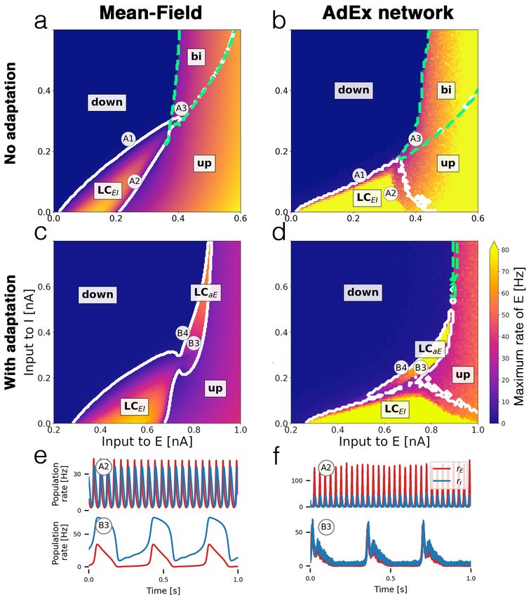
Cakan et al. 5/40Fig 3. Transition from multistability to slow oscillation is caused by
somatic adaptation. Bifurcation diagrams depending on the external input current
C · µext
α to both populations α ∈ {E, I} for varying somatic adaptation parameters a
and b. Color indicates maximum rate of the excitatory population. Oscillatory regions
have a white contour, bistable regions have a green dashed contour. (a) Bifurcation
diagrams of the mean-field model. On the diagonal (bright-colored diagrams),
adaptation parameters coincide with (b). (b) Bifurcation diagrams of the corresponding
AdEx network, N = 20 × 103 . All parameters are listed in Table 1.
Cakan et al. 6/40The bifurcation diagrams in Fig. 3 show how the emergence of the slow oscillation
depends on the adaptation mechanism. Increasing the subthreshold adaptation parameter
primarily shifts the state space to the right whereas a larger spike-triggered adaptation
parameter value enlarges oscillatory regions. Both parameters cause the bistable region
to shrink until it is eventually replaced by a slow oscillatory region LCaE . Again, the
state space of the mean-field model (Fig. 3 a) reflects the AdEx network (Fig. 3 b)
accurately.
Time-varying stimulation and electric field effects
To describe the time-dependent properties of the system, we study the effects of time-
varying external stimulation and the interactions with ongoing oscillatory states. External
stimulation is implemented by coupling an electric input current to the excitatory
population. This additional input current may be a result of an externally applied
electric field or synaptic input from other neural populations. For the cases without
adaptation, we can calculate an equivalent extracellular electric field strength that
correspond to the effects of an input current (see Methods).
Since due to the presence of apical dendrites, excitatory neurons in the neocortex
are most susceptible to electric fields [32], only time-varying input to the excitatory
population is considered. This choice is also motivated in the context of inter-areal brain
network models where connections between brain areas are usually considered between
excitatory subpopulations.
Given the multitude of possible states of the system, its response to external input
critically depends on the dynamical landscape around its current state. It is important
to keep in mind that the bifurcation diagrams (Figs. 2 and 3) are valid only for constant
external input currents. However, they provide a helpful estimation of the dynamics of
the non-stationary system assuming that the bifurcation diagrams do not change too
much as we vary the input parameter µext e (t) over time.
Figs. 4 a-f show how a step current input pushes the system in and out of specific
states of the E-I system. A positive step current represents a movement in the positive
direction of the µext
e -axis in Fig. 2. Figs. 4 a and b show input-driven transitions from
the low-activity down-state to the fast oscillatory limit cycle LCEI . Similar behavior
can be observed in Figs. 4 c and d where we push the system’s state from LCEI to the
up-state, effectively being able to turn oscillations on and off with a direct input current.
Inside the bistable region, we can use the hysteresis effect to transition between
the down-state and the up-state and vice versa. After application of an initial push in
the desired direction, the system remains in that state, reflecting the system’s bistable
nature.
With adaptation turned on, a slow oscillatory input current can entrain the ongoing
oscillation. In Figs. 4 g and h, the oscillation is initially out of phase with the external
input but is quickly phase-locked. Placed close to the boundary of the slow oscillatory
region LCaE , we show in Figs. 4 i and j how an oscillatory input with a similar frequency
as the limit cycle periodically drives the system from the down-state into one oscillation
period.
Close inspection of Fig. 4 b shows that the fast oscillation in the AdEx network has
a varying amplitude, in contrast to the mean-field model Fig. 4 a. This difference is due
to noise resulting from the finite size of the AdEx network and decreases as the network
size N increases. (see Fig. S16) All of the state transitions take longer for the AdEx
network, as it is visible in Fig. 4 d for example. Additionally, transitions to the up-state
and the slow limit cycle LCaE are accompanied by transient ringing activity (Figs. 4 f
and h), which is not well-captured by the mean-field model.
Cakan et al. 7/40Fig 4. State-dependent population response to time-varying input currents.
Population rates of the excitatory population (black) with an additional external
electrical stimulus (red) applied to the excitatory population. (a, b) A DC step input
with amplitude 60 pA (equivalent E-field amplitude: 12 V/m) pushes the system from
the low-activity fixed point into the fast limit cycle LCEI . (c, d) A step input with
amplitude 40 pA (8 V/m) pushes the system from LCEI into the up-state. (e, f ) In the
multistable region bi, a step input with amplitude 100 pA (20 V/m) pushes the system
from the down-state into the up-state and back. (g ,h) Inside the slow oscillatory region
LCaE , an oscillating input current with amplitude 40 pA and a (frequency-matched)
frequency of 3 Hz phase-locks the ongoing oscillation. (i, j) A slow 4 Hz oscillatory
input with amplitude 40 pA drives oscillations if the system is close to the oscillatory
region LCaE . For the AdEx network, N = 100 × 103 . All parameters are given in Table
1, the parameters of the points of interest are given in Table 2.
Cakan et al. 8/40Frequency entrainment with oscillatory input
To study the frequency-dependent response of the E-I system, we vary the amplitude and
frequency of an oscillatory input to the excitatory population (Fig. 5). The unperturbed
system is parameterized to be in the fast limit cycle LCEI with its endogenous frequency
f0 .
The external stimulus with frequency fext entrains the ongoing oscillation in a range
around f0 , the resonant frequency of the system. Here, the ongoing oscillation essentially
follows the external drive and adjusts its frequency to it (Fig. 5 a). A second (narrower)
range of frequency entrainment appears as fext approaches 2f0 , representing the ability
of the input to entrain oscillations at half of its frequency. Due to interference of the
frequencies of ongoing and external oscillations, the spectrum has peaks at the difference
of both frequencies which appear as X-shaped patterns in the frequency diagrams. The
AdEx network shows a similar behavior (Fig. 5 b), albeit the range of entrainment is
smaller than in the mean-field model, despite the stimulation amplitude being twice as
large.
For stronger oscillatory input currents, the range of frequency entrainment is widened
considerably. In Fig. 5 c and d, the input dominates the spectrum at very low frequencies.
The peak of the spectrum reverts back to approximately f0 if the external frequency
fext is close to the first harmonic 2f0 of the endogenous frequency. We see multiple lines
emerging in the frequency spectra which correspond to the harmonics and subharmonics
of the external frequency and its interaction with the endogenous frequency f0 , creating
complex patterns in the diagrams. Differences between the spectrograms of the AdEx
network in Fig. 5 d and the mean-field model Fig. 5 c can be largely attributed to the
fact that the AdEx network consistently needs stronger inputs to obtain the same effect
as in the mean-field model. This results in horizontal lines in areas where frequency
entrainment is not effective and in faint and short diagonal lines between the lines that
represent the (sub-)harmonics which are caused by interactions with the (sub-)harmonics.
In the mean-field model, we mainly observe clear diagonal lines, indicating successful
entrainment. Another source for the differences is the inherently noisy dynamics of the
AdEx network, due to its finite size (see Fig. S16).
Overall, there is a good qualitative agreement of the frequency spectra of both models,
reflecting that interactions of time-varying external inputs and ongoing oscillations are
well-represented by the mean-field model.
Phase locking with oscillatory input
Here we quantify the ability of an oscillating external input current to the excitatory
population to synchronize an ongoing neural oscillation to itself if both frequencies, the
driver and the endogenous frequency, are close to each other (frequency matching). An
example time series of a stimulus entraining an ongoing slow oscillation is shown in Fig.
4 h.
In Fig. 6, we find phase locking by measuring the time course of the phase difference
between the stimulus and the population rate. If phase locking is successful, the phase
difference remains constant. In Fig. 6 a, the region of phase locking for an external input
of frequency fext is centered around the endogenous frequency f0 of the unperturbed
system. Increasing the stimulus amplitude widens the range around f0 at which phase
locking is effective, producing Arnold tongues in the diagram. An example time series of
successful phase locking inside this region is shown in Fig 6 c at point 1. If the input
is not able to phase-lock the ongoing activity, a small difference between the driver
frequency fext and f0 can cause a slow beating of the activity with a frequency of roughly
the difference |fext − f0 |. Thus, a small frequency mismatch can produce a very slowly
oscillating activity (Fig. 6 c at points 2-4). Figure 6 d at point 2 shows the same drifting
Cakan et al. 9/40Fig 5. Frequency entrainment of the population activity in response to
oscillatory input. The color represents the log-normalized power of the excitatory
population’s rate frequency spectrum with high power in bright yellow and low power in
dark purple. (a) Spectrum of mean-field model parameterized at point A2 with an
ongoing oscillation frequency of f0 = 22 Hz (horizontal green dashed line) in response to
a stimulus with increasing frequency and an amplitude of 20 pA. An external electric
field with a resonant stimulation frequency of f0 has an equivalent strength of 1.5 V/m.
The stimulus entrains the oscillation from 18 Hz to 26 Hz, represented by a dashed green
diagonal line. At 27 Hz, the oscillation falls back to its original frequency f0 . At a
stimulation frequency of 2f0 , the ongoing oscillation at f0 locks again to the stimulus in
a smaller range from 43 Hz to 47 Hz. (b) AdEx network with f0 = 30 Hz. Entrainment
with an input current of 40 pA is effective from 27 Hz to 33 Hz. Electric field amplitude
with frequency f0 corresponds to 2.5 V/m. (c) Mean-field model with a stimulus
amplitude of 100 pA (7.5 V/m at 22 Hz). Green dashed lines mark the driving frequency
fext and its first and second harmonics f1H and f2H and subharmonics f1SH and f2SH .
Entrained is now effective at the lowest stimulation frequencies until at 36 Hz the
oscillation falls back to a frequency of 20 Hz. New diagonal lines appear due to
interactions of the endogenous oscillation with the entrained harmonics and
subharmonics. (d) AdEx network with stimulation amplitude of 140 pA (8.75 V/m at 30
Hz). For the AdEx network, N = 20 × 103 . All parameters are given in Tables 1 and 2.
Cakan et al. 10/40Fig 6. Phase locking of ongoing oscillations via weak oscillatory inputs. The
left panels show heatmaps of the level of phase locking for (a) the mean-field model and
(b) the AdEx network for different stimulus frequencies and amplitudes. Dark areas
represent effective phase locking and bright yellow areas represent no phase locking.
Phase locking is measured by the standard deviation of the Kuramoto order parameter
R(t) which is a measure for phase synchrony. White dashed lines correspond to electric
field with equivalent strength in V/m. (c) Time series of four points indicated in (a)
with the excitatory population’s rate in black and the external input in red (upper
panels). In the lower panels, the Kuramoto order parameter R(t) is shown, measuring
the synchrony between the population rate and the external input. Constant R(t)
represents effective phase locking (phase difference between rate and input is constant),
fluctuating R(t) indicates dephasing of both signals, hence no phase locking. (d)
Corresponding time series of points in (b). Both models are parameterized to be in point
A2 inside the fast oscillatory region LCEI . Insets show zoomed-in traces from 15 to 16
seconds. For the AdEx network, N = 20 × 103 . All parameters are given in Table 1.
Cakan et al. 11/40effect in the AdEx network. Due to finite-size noise in the AdEx network, an irregular
switching between synchrony and asynchrony can be observed at the edges of the phase
locking region in Fig. 6 d at point 3. Compared to the mean-field model, the frequency
of the beating activity in the AdEx network is less regular (Fig. 6 d at point 4).
In the phase locking diagrams Figs. 6 a and b, the equivalent external electric field
amplitudes are shown. Small amplitudes (0.2 V/m for the mean-field model, 0.5 V/m
for the AdEx network) are able to phase-lock the ongoing oscillations if the frequencies
roughly match.
Discussion
In this paper, we explored the dynamical properties of a cortical neural mass model of
excitatory and inhibitory (E-I) adaptive exponential integrate-and-fire (AdEx) neurons
by studying their response to external electrical stimulation. Results from a low-
dimensional mean-field model of a spiking AdEx neuron network were compared with
large network simulations (Fig. 1). The mean-field model provides an accurate and
computationally efficient approximation of the mean population activity and the mean
membrane potentials of the AdEx network if all neurons are equal, the number of neurons
is large, and the connectivity is sparse and random. The mean-field model and the AdEx
network share the same set of biophysical parameters (see Methods). The biophysical
parameters of the AdEx neuron allow us to model realistic external electric currents and
extracellular field strengths [28]. In the mean-field description, this allows us to model
stimulation to the whole population in various network states.
Bifurcation diagrams (Figs. 2) provide a map of the possible states as a function
of the external inputs to both, excitatory and inhibitory, populations. A comparison
of the diagrams of the mean-field model to the corresponding AdEx network model
reveals a high degree of similarity of the state spaces. Each attractor of the AdEx
network is represented in the mean-field model in a one-to-one fashion which allows for
accurate predictions of the state of the spiking neural network using the low-dimensional
mean-field model.
We have focused our attention on bifurcations caused by changes of the mean
external input currents which can represent background inputs to the neural population
or electrical inputs from external stimulation. It is worth noting that other parameters,
such as coupling strengths and adaptation parameters, can cause bifurcations as well.
Overall, the specific shape of the dynamical landscape depends on numerous parameters.
However, extensive parameter explorations indicated that the accuracy of the mean-field
model as well as the overall structure of the bifurcation diagrams presented in this paper
was fairly robust to changes of the coupling strengths and therefore representative for
this E-I system (see Figs. S13 and S14).
Without a somatic adaptation feedback mechanism, the population rate can occupy
four distinct states: a down-state with very low activity, an up-state with constant
high activity representing an asynchronous firing state of the neurons (see Fig, S9), a
bistable regime where down-state and up-state coexist and an oscillatory state where
the activity alternates between the excitatory and the inhibitory population at a low
gamma frequency.
Somatic adaptation causes slow network oscillations
The AdEx neuron model allows for incorporation of a slow potassium-mediated adaptation
current, typically found in cortical pyramidal neurons [33]. Due to somatic adaptation,
in the bistable region, the up-state loses its stability. The bistable region transforms
into a second oscillatory regime (Fig. 3) in which the population activity oscillates
Cakan et al. 12/40at low frequencies between 0.5 Hz and 5 Hz. This oscillatory region coexists with the
fast excitatory-inhibitory oscillation. Other computational studies have focused on the
origin of this adaptation-mediated oscillation [29–31], the interaction of adaptation with
noise-induced state switching between up- and down-state [29,34,35] and how adaptation
affects the intrinsic timescales of the network [36, 37].
Electric field effects and relation to experimental observations
Using the bifurcation diagrams (Fig. 2), we mapped out several points of interest
that represent different network states. The type of reaction to external stimulation
depends on the current state of the system, as seen in the population time series during
stimulation in Fig. 4. Close to edges of attractors, direct currents can cause bifurcations
and trigger a sudden change of the dynamics, such as transitions from a low activity
down-state to a state with oscillatory activity.
In vitro stimulation experiments with electric fields [3] have shown that (time-constant)
direct fields are able to switch on and off oscillations at field strengths of 6 V/m. In Fig.
4, we could observe this at 8 −12 V/m, when the system if placed close to the oscillatory
state. This difference in amplitudes can be attributed to the chosen initial state of the
system and could be reduced if the background inputs were parameterized closer to the
limit cycle.
Inside oscillatory regions, oscillatory input causes phase locking and frequency en-
trainment. Frequency entrainment is the ability of an external stimulus to force the
endogenous oscillation to follow its frequency. To study how frequency entrainment
depends on the frequency and amplitude of the stimulus, we analyzed frequency spec-
trograms of the population activity when subject to external oscillating stimuli with
increasing frequencies (Fig. 5). We observed shifts of the peak frequency around the
endogenous frequency at amplitudes corresponding to field strengths of 1.5 V/m in the
mean-field model and 2.5 V/m in the AdEx network. Similar effects have been reported
in in vitro experiments, where the frequency of the ongoing oscillations changed along
with the stimulus frequency [3, 38–40].
Interestingly, the field amplitudes at which frequency entrainment is visible are on
the same order of endogenous fields in the brain, generated by the neural activity itself.
Electrophysiological experiments show that these fields can be as strong as 3.5 V/m [11]
and that ephaptic coupling plays a significant role in the brain [12]. Our findings support
this observation from a theoretical perspective, since one of our main results is that
considerable effects on the population dynamics are expected at these field strengths.
We also observed frequency entrainment of the subharmonics of the endogenous
oscillation as it was shown in in vitro experiments in Refs. [3, 39] and its harmonics in
Ref. [38]. This effect could be valuable for experimental conditions where it is impractical
to use stimulation frequencies close to the endogenous frequency of ongoing oscillations
in the studied neural system. The range of frequency entrainment around the natural
frequency of the endogenous oscillation widens as the stimulus amplitude increases,
which was also observed in similar computational studies [41, 42].
If the stimulus frequency is close to the endogenous frequency (frequency matching),
an oscillatory stimulus can force the ongoing oscillation to synchronize its phase with
the stimulus, known as phase locking, phase entrainment, or coherence. Phase locking
of ongoing brain activity to a stimulus has been observed in multiple noninvasive
brain stimulation studies, including Refs. [43–45], and it has been shown to affect
information processing properties of the brain [7, 8] as particularly sensory information
processing depends on phase coherence of oscillations between distant brain regions [46,47].
Compared to frequency entrainment, very weak input currents are able to phase lock
ongoing oscillations. In agreement with these experiments, we find phase locking to
be effective at electric field strengths of around 0.5 V/m (Fig. 6), which is in the
Cakan et al. 13/40range of typical field strengths generated by transcranial alternating current stimulation
(tACS) [48].
To summarize: Our results confirm the interesting notion that, while weak electric
fields with strengths in the order of 1 V/m that are typically applied in tACS experiments
have only a small effect on the membrane potential of a single neuron [32], the effects on
the network however, and therefore on the dynamics of the population as a whole, can
be quite significant, which was also observed experimentally [49]. This indicates that
field effects are strongly amplified in the network. Considering slightly stronger fields,
our results suggest that endogenous fields, generated by the activity of the brain itself,
are expected to have a considerable effect on neural oscillations, facilitating phase and
frequency synchronization across neighboring cortical brain areas.
Validity of the mean-field method and limitations of our approach
We found all observed input-dependent effects in the AdEx network to be well-represented
by the mean-field model, which demonstrates its accuracy also in the non-stationary
case. However, partly due to the difference of parameters that define the states in the
bifurcation diagrams, the AdEx network consistently requires larger input amplitudes in
order to cause the same effect size as observed in the mean-field model (Figs. 5 and 6).
Although it was not investigated here, we hypothesize that the number of neurons might
play an important role in how much external inputs are amplified within a network.
Related to this is the fact that our approximation assumes the number of neurons
to be infinitely large. Therefore, differences between the mean-field model and the
AdEx network in the case without external stimulation also depend on the network
size. However, we find good agreement between the bifurcation diagrams for as low
as N = 4 × 10³ neurons (Fig. S15). With increasing network size, the amplitudes of
oscillations in the AdEx network shown in Fig. 4 b approach the predictions of the
mean-field model and become less irregular (Fig. S16).
Comparing the bifurcation diagrams of both models (Fig. 2), the shape of the
oscillatory region as well as the frequencies of the oscillations differ (see Fig. S12). We
suspect that the oscillatory states are where the steady-state approximations that are
used to construct the mean-field model break down due to the fast temporal dynamics in
this state. Hence, both models have notable differences between the oscillatory regions.
Sharp transitions between states cause transient effects that are visible as ringing
oscillations in the population firing rate, typically observed in simulations of spiking
networks (such as in Fig. 4 f and h) or experimentally [50]. The poor reproduction of
these oscillations in our model is likely due to the use of an exponentially-decaying linear
response function instead of a damped oscillation which would be a better approximation
of the true response (c.f. Ref. [23]). This constitutes a possible improvement of our work.
Recent advancements in mean-field models of cortical networks [51] can account for its
finite size as well as reproduce transient oscillations caused by sharp input onsets.
Another important limitation of our method is the assumption of homogeneous
and weak synaptic coupling in the mathematical derivation of our mean-field model.
Synapses in the brain are known to be log-normally distributed [52] with long tails,
implying the existence of few but strong synapses. Other computational papers have
specifically focused on the effect of strong synapses on the population activity (cf. [53]
and [54]). Therein, the incorporation of strong synapses causes the emergence of a new
asynchronous state in which the firing rates of individual neurons fluctuate strongly,
similar to chaotic states studied in networks of rate neurons [55], which are qualitatively
different from the up-state that we observed (see Fig. S9). In Ref. [53], the author shows
that firing rate models similar to what we consider break down and cannot capture the
large fluctuations present in this state. We therefore conclude that our mean-field model
is limited to describing only weak synaptic coupling.
Cakan et al. 14/40Furthermore, a number of assumptions were made in our model of electric field inter-
action. Most importantly, we have chosen typical morphological and electrophysiological
parameters of a ball-and-stick neuron model to represent pyramidal cells in layer 4/5 of
cortex (see Methods). Despite the simplicity of the ball-and-stick model, it was shown in
Ref. [28] that it can reproduce the somatic polarization of a pyramidal cell in a weak and
uniform field. This was then translated into effective input currents to point neurons
which lack any morphological features. In addition to the crude assumption that all
neurons have the same simple morphology (effects of a more complex morphology were
studied in Ref. [56]), we also assumed perfect alignment of the dendritic cable to the
external electric field. While the latter might be a good approximation for a local region
of the cortex it is not the case for the brain as a whole with its folded structure. It has
been shown that the somatic polarization of a neuron strongly depends on the angle
between the neuron’s main axis and the electric field [32].
We only focused on field effects that are caused by the dendrite. Although we expect
that, in principle, axons could contribute to the somatic polarization in a weak and
uniform electric field, their contribution could be relatively small, since most cortical
axons are not geometrically aligned with each other the way that dendrites are organized
in the columnar structure of the cortex [57].
Finally, we assumed that the field effects are only subthreshold such that our results
do not generalize to stimulation scenarios with strong electric fields that can elicit action
potentials by themselves.
Conclusion
Overall, our observations confirm that a sophisticated mean-field model of a neural
mass is appropriate for studying the macroscopic dynamics of large populations of
spiking neurons consisting of excitatory and inhibitory units. To our knowledge, such a
remarkable equivalence of the dynamical states between a mean-field neural mass model
and its ground-truth spiking network model has not been demonstrated before. Our
analysis shows that mean-field models are useful for quickly exploring the parameter
space in order to predict states and parameters of the neural network they are derived
from. Since the dynamical landscapes of both models are very similar, we believe that it
should be possible to reproduce a variety of stationary and time-dependent properties of
large-scale network simulations using low-dimensional population models. This may help
to mechanistically describe the rich and plentiful observations in real neural systems
when subject to stimulation with electric currents or electric fields, such as switching
between bistable up and down-state or phase locking and frequency entrainment of the
population activity.
Bifurcations, as studied in dynamical systems theory, offer a plausible mechanism of
how networks of neurons as well as the brain as a whole [58, 59] can change its mode of
operation. Understanding the state space of real neural systems could be beneficial for
developing electrical stimulation techniques and protocols, represented as trajectories in
the dynamical landscape, which could be used to reach desirable states or specifically
inhibit pathological dynamics.
Due to the variety of possible macroscopic network states that arise from this basic
E-I architecture, it is critical to consider the state of the system in order to comprehend
and predict its response to external stimuli. This might explain the numerous seemingly
inconclusive experimental results from noninvasive brain stimulation studies [5,6] where it
is hard to account for the state of the brain before stimulation. In conclusion, additional
to the stimulus parameters, the response of a system to external stimuli has to be
understood in context of the dynamical state of the unperturbed system [3, 42, 60].
Cakan et al. 15/40Materials and methods
Neural population setting
In order to derive the mean-field description of an AdEx network, we consider a very
large number of N → ∞ neurons for each of the two populations E and I. We assume (1)
random connectivity (within and between populations), (2) sparse connectivity [61, 62],
but each neuron having a large number of inputs [63] K with 1
K
N , (3) and that
each neuron’s input can be approximated by a Poisson spike train [64, 65] where each
incoming spike causes a small (c/J
1) and quasi-continuous change of the postsynaptic
potential (PSP) [66] (diffusion approximation).
The spiking neuron model
The adaptive exponential (AdEx) integrate-and-fire neuron model forms the basis for
the derivation of the mean-field equations as well as the spiking network simulations.
Each population α ∈ {E, I} has Nα neurons which are indexed with i ∈ [1, Nα ]. The
membrane voltage of neuron i in population α is governed by
dVi
C = Iion (Vi ) + Ii (t) + Ii,ext (t), (1)
dt
V − VT
Iion (V ) = gL (EL − V ) + gL ∆T exp − IA (t). (2)
∆T
The first term of Iion (Eq. 2) describes the voltage-depended leak current, the second
term the nonlinear spike initiation mechanism, and the last term IA , the somatic
adaptation current. Ii,ext (t) = µext (t) + σ ext ξi (t) is a noisy external input. It consists of
a mean current µext (t) which is equal across all neurons of a population and independent
Gaussian fluctuations ξi (t) with standard deviation σ ext (σ ext is equal for all neurons of
a population). For a neuron in population α, synaptic activity induces a postsynaptic
current Ii which is a sum of excitatory and inhibitory contributions:
Ii (t) = C(JαE si,αE (t) + JαI si,αI (t)), (3)
with C being the membrane capacitance and Jαβ the coupling strength from population
β to α, representing the maximum current when all synapses are active. The synaptic
dynamics is given by
dsi,αβ si,αβ cαβ X X
=− + (1 − si,αβ ) Gij δ(t − tkj − dαβ ). (4)
dt τs Jαβ j k
si,αβ (t) represents the fraction of active synapses from population β to α and is bound
between 0 and 1. Gij is a random binary connectivity matrix with a constant row sum
Kα and connects neurons j of population β to neurons i of population α. With the
constraint of a constant in-degree Kα of each unit, all neurons of population β project
to neurons of population α with a probability of pαβ = Kα /Nβ and α, β ∈ {E, I}. Gij is
generated independently for every simulation. The first term in Eq. 4 is an exponential
decay of the synaptic activity, whereas the second term integrates all incoming spikes
as long as si,αβ < 1 (i.e. some synapses are still available). The first sum is the sum
over all afferent neurons j, and the second sum is the sum over all incoming spikes k
from neuron j emitted at time tk after a delay dαβ . If si,αβ = 0, the amplitude of the
postsynaptic current is exactly C · cαβ which we set to physiological values from in vitro
measurements [67] (see Table 1).
Cakan et al. 16/40For neurons i of the excitatory population, the adaptation current IA,i (t) is given by
dIA,i
τA = a(Vi − EA ) − IA,i , (5)
dt
a representing the subthreshold adaptation and b the spike-dependent adaptation pa-
rameters. The inhibitory population doesn’t have an adaptation mechanism, which is
equivalent to setting these parameters to 0. When the membrane voltage crosses the
spiking threshold, Vi ≥ Vs , the voltage is reset, Vi ← Vr , clamped for a refractory time
Tref , and the spike-triggered adaptation increment is added to the adaptation current,
IA,i ← IA,i + b. All parameters are given in Table 1.
Finally, we define the mean firing rate of neurons in population α as
αN Z t+dt
1 1 X
rα (t) = δ(t0 − tki )dt, (6)
Nα dt i=0 t
which measures the number of spikes in a time window dt, set to the integration step
size in our numerical simulations.
The mean-field neural mass model
For a sparsely connected random network of AdEx neurons as defined by Eqs. 1-5, the
distribution of membrane potentials p(V ) and the mean population firing rate r can be
calculated using the Fokker-Planck equation in the thermodynamic limit N → ∞ [13,68].
Determining the distribution involves solving a partial differential equation, which is
computationally demanding. A low-dimensional linear-nonlinear cascade model [24, 69]
can be used to capture the steady-state and transient dynamics of a population in form
of a set of simple ODEs. Briefly, for a given mean membrane current µα with standard
deviation σα , the mean of the membrane potentials V̄α as well as the population firing
rate rα in the steady-state can be calculated from the Fokker-Plank equation [70] and
captured by a set of simple nonlinear transfer functions Φ(µα , σα ) (shown in Figs. 7 a
and b).
These transfer functions can be precomputed (once) for a specific set of single AdEx
neuron parameters. All other parameters, such as input currents, network parameters
and synaptic coupling strengths, as well as the parameters that govern the somatic
adaptation mechanism, the membrane timescale, and the synaptic timescale are identical
and directly represented in the equations of the mean-field model. Thus, for any given
parameter configuration of the AdEx network, there is a direct translation to the
parameters that define the mean-field model. This also allows for direct comparison of
both models under changes of said parameters.
The reproduction accuracy of the linear-nonlinear cascade model for a single popula-
tion has been systematically reviewed in Ref. [23] and has been shown to reproduce the
dynamics of an AdEx network in a range of different input regimes quite successfully,
while offering significant increase in computational efficiency.
Rate equations
The derivation of the equations that govern the mean µα and variance σα2 of the membrane
currents, the mean adaptation current I¯A , and the mean s̄αβ and variance σs, 2
αβ
of the
synaptic activity are presented further below. The full set of equations of the mean-field
model reads:
Cakan et al. 17/40Fig 7. Precomputed quantities of the linear-nonlinear cascade model. (a)
Nonlinear transfer function Φ for the mean population rate (Eq. 15) (b) Transfer
function for the mean membrane voltage (Eq. 10) (c) Time constant τα of the linear
filter that approximates the linear rate response function of AdEx neurons (Eq. 7). The
color scale represents the level of the input current variance σα across the population.
All neuronal parameters are given in Table 1.
dµα
τα = µsyn ext
α (t) + µα (t) − µα (t), (7)
dt
µsyn
α (t) = JαE s̄αE (t) + JαI s̄αI (t), (8)
X 2Jαβ 2 2
σs,αβ (t) τs,β τm
σα2 (t) = 2
+ σext,α , (9)
(1 + rαβ (t)) τm + τs,β
β∈{E,I}
dI¯A
= τA−1 a(V̄E (t) − EA ) − I¯A + b · rE (t),
(10)
dt
ds̄αβ −1
= −τs,β s̄αβ (t) + 1 − s̄αβ (t) · rαβ (t), (11)
dt
2
dσs,αβ 2 −2
2
= 1 − s̄αβ (t) · ραβ (t) + τs,β (ραβ (t) − 2τs,β (ραβ (t) + 1 · σs,αβ (t), (12)
dt
for α, β ∈ {E, I}. All parameters are listed in Table 1. The mean rαβ and the variance
ραβ of the effective input rate from population β to α for a spike transmission delay dαβ
are given by
cαβ
rαβ (t) = Kβ · rβ (t − dα ), (13)
Jαβ
cαβ
ραβ (t) = · rαβ (t). (14)
Jαβ
rα is the instantaneous population spike rate, cαβ defines the amplitude of the post-
synaptic current caused by a single spike (at rest, sαβ = 0) and Jαβ sets the maximum
membrane current generated when all synapses are active (at sαβ = 1).
To account for the transient dynamics of the population to a change of the membrane
currents, µα can be integrated by convolving the input with a linear response function.
This function is well-approximated by a decaying exponential [23, 24, 69] with a time
constant τα (shown in Fig. 7 c). Thus, the convolution can simply be expressed as an
ODE (Eq. 7) with an input-dependent adaptive timescale τα that is updated at every
integration timestep. In Eq. 7, µsyn
α (t), as defined by Eq. 8, represents the mean current
caused by synaptic activity and µext
α (t) the currents caused by external input.
The instantaneous population spike rate rα is determined using the precomputed
nonlinear transfer function
rα = Φ(µα , σα ). (15)
Cakan et al. 18/40The transfer function Φ is shown in Fig. 7 a. It translates the mean µα as well as the
standard deviation σα (Eq. 9) of the membrane currents to a population firing rate.
Using an efficient numerical scheme [24, 70], this function was previously computed [23]
from the steady-state firing rates of a population of AdEx neurons given a particular
input mean and standard deviation. The transfer function depends on the parameters
of the single AdEx neuron. Equation 10 governs the evolution of the mean adaptation
current of the excitatory population. Equations 11 and 12 describe the mean and the
standard deviation of the fraction of active synapses caused by incoming spikes from
population β to population α.
Synaptic model
Following Ref. [71], we derive ODE expressions for the population mean s̄αβ and variance
2
σs,αβ of the synaptic activity. We rewrite the synaptic activity given by Eq. 4 of a
neuron i from population α caused by inputs from population β with α, β ∈ {E, I} in
terms of a continuous input rate rβ (diffusion approximation) such that
dsi,αβ cαβ
q
τs,β = −si + (1 − si ) Kα rβ (t − dα ) + Kα rβ (t − dα )ξi (t) , (16)
dt Jαβ
P
with Kα = j∈α Gij being the constant in-degree of each neuron, rβ (t−dα ) the incoming
delayed mean spike rate from all afferents of population β, and ξi (t) being standardized
Gaussian white noise. The current Ii (t) of a neuron in population α due to synaptic
activity is given by
X
Ii (t) = CJαβ si,αβ (t). (17)
β∈{E,I}
We split the mean from the variance of Eq. 16 by first taking the mean over neurons of
Eq. 16. The mean synaptic activity s̄αβ := hsi,αβ ii of population α caused by input from
population β is then given by Eq. 11. We get the differential equation of the variance
2
σs,αβ of si,αβ in Eq. 12 by applying Ito’s product rule [72] on d(s2i,αβ ) and taking its
time derivative.
Input currents
Additional to the mean currents (Eq. 7) in the population, we also keep track of their
variance. Figure 7 shows the population firing rate and mean membrane potential for
different levels of variance of the membrane currents. Especially the adaptive time
constant τα , which affects the temporal dynamics of the population’s response, strongly
depends on the variance of the input. Please note that the adaptive time constant τα is
not related to the somatic adaptation mechanism. Without loss of generality, we derive
the variance of the membrane currents caused by a single afferent population α and
later add up the contributions of two coupled populations (excitatory and inhibitory).
Assuming that every neuron receives a large number of uncorrelated inputs (white noise
approximation), we write the synaptic current Ii,α (t) in terms of contributions to the
population mean and the variance [13, 73–76]:
Ii,α (t) = C µα (t) + σα (t)ξi (t) . (18)
In order to obtain the contribution of synaptic input to the mean and the variance
of membrane currents, we (1) neglect the exponential term of Iion in Eq. 2 and (2)
assume that the membrane voltages are mostly subthreshold such that we can neglect
the nonlinear reset condition. Numerical simulations have proven that these assumptions
Cakan et al. 19/40are justifiable in the parameter ranges that we are concerned with [71]. We apply these
simplifications only in this step of the derivation. The exponential term, the neuronal
parameters within it, and the reset condition still affect the precomputed functions
(shown in Fig. 7) and thus the overall population dynamics.
We substitute both approximations Eq. 17 and Eq. 18 separately into the membrane
voltage Eq. 1 and apply the expectation operator on both sides, which leads to two
equations describing the evolution of the mean membrane potential. If we require that
both approximations should yield the same mean potential hVi,α i, we can easily see that
µsyn 2
α (t) = Jαα hsi,αα (t)i. Using Ito’s product rule [72] on dV and requiring that both
approximations should also result in the same evolution of the second moment hVα2 i, we
get
σα2 (t) = 2Jαα hVi,α si,αα i − hVi,α ihsi,αα i .
(19)
Taking the time derivative of Eq. 19 and substituting the time derivative of hVα sαα i by
applying Ito’s product rule on d(Vα sαα ) we obtain
dσα2 2 2 cτα Krαα (t) + 1 1 2
= 2Jαα σs,αα (t) − + σ (t) (20)
dt τs,α τm s,αα
2
Here, σs,αα := hs2i,αα i − hsi,αα i2 . The timescale of Eq. 20 is much smaller than τα of Eq.
7. We can therefore approximate σα2 (t) well with its steady-state value:
2 2
2Jαα τm τα σs,αα (t)
σα2 (t) = , (21)
(cτα Krαα (t) + 1)τm + τs,α
τm = C/gL being the membrane time constant. Adding up the variances in Eq. 21 of
2
both E and I subpopulations and the variance of the external input σext,α , the total
variance of the input currents is then given by Eq. 9. The two moments of the membrane
currents, µα and σα , fully determine the instantaneous firing rate rα = hri ii (Eq. 15),
the mean membrane potential V̄α := hVi ii , and the adaptive timescale τα (Fig. 7).
Adaptation mechanism
The large difference of timescales of the slow adaptation mechanism mediated through
K+ channel dynamics compared to the faster membrane voltage dynamics [77,78] and the
synaptic dynamics allows for a separation of timescales [37] (adiabatic approximation).
Therefore, each neuron’s adaptation current can be approximated by its population
average I¯A , which evolves according to Eq. 10, where a is the sub-threshold adaptation
and b is the spike-triggered adaptation parameter. V̄α (t) = V̄α (µα , σα ) is the mean of
the membrane potentials of the population and was precomputed and is read from a
table (Fig. 7 b) at every timestep. In the case of a, b > 0, i.e. when adaptation is active,
we subtract the current I¯A caused by the adaptation mechanism from the current C · µα
caused by the synapses in order to obtain the net input current. The resulting firing rate
of the excitatory population is then determined by evaluating rE = Φ(µE − I¯A /C, σE ).
For inhibitory neurons, adaptation was neglected (a = b = 0) since the adaptation
mechanism was found to be much weaker than in the case of excitatory pyramidal
cells [79].
Obtaining bifurcation diagrams and determining bistability
Each point in the bifurcation diagrams in Figs. 2 and 3 was simulated for pairs of
external inputs µext ext
E and µI and the resulting time series of the excitatory population
rate of the mean-field model and the AdEx network were analyzed and the dynamical
state was classified.
Cakan et al. 20/40You can also read