Jobs and Matches: Quits, Replacement Hiring, and Vacancy Chains
←
→
Page content transcription
If your browser does not render page correctly, please read the page content below
AER: Insights 2020, 2(1): 101–124
https://doi.org/10.1257/aeri.20190023

                   Jobs and Matches: Quits, Replacement Hiring,
                              and Vacancy Chains†
                               By Yusuf Mercan and Benjamin Schoefer*

                 In the canonical DMP model of job openings, all job openings stem
                 from new job creation. Jobs denote worker-firm matches, which are
                 destroyed following worker quits. Yet, employers classify 56 percent
                 of vacancies as quit-driven replacement hiring into old jobs, which
                 evidently outlived their previous matches. Accordingly, aggregate
                 and firm-level hiring tightly track quits. We augment the DMP model
                 with longer-lived jobs arising from sunk job creation costs and
                 replacement hiring. Quits trigger vacancies, which beget vacancies
                 through replacement hiring. This vacancy chain can raise total job
                 openings and net employment. The procyclicality of quits can thereby
                 amplify business cycles. (JEL E24, E32, J23, J31, J63)

          In matching models of the labor market, firms post vacancies to recruit workers
       into newly created jobs. A job is a match between a particular worker and particular
       firm, and disappears whenever that first match dissolves. This paper studies a more
       realistic notion of longer-lived jobs that outlive matches. Job openings then com-
       prise new jobs as well as reposted old jobs.
          A central and motivating contribution of this paper is our new, direct job-level
       evidence for replacement hiring: 56 percent of real-world job vacancies are for old
       jobs vacated by quits—rather than 100 percent new job creation as in the standard
       model. Our source is the IAB Job Vacancy Survey, in which German employers
       directly classify the nature of a given job opening, distinguishing such replace-
       ment hiring from creation of a new job. This composition is masked in standard,
       catch-all measures of vacancies. In an event study design, we estimate that at the
       establishment level, one incremental quit triggers almost perfect replacement hiring.
          In the aggregate, quits, which are dramatically procyclical, comove nearly one
       to one with hires and job openings. Our paper explores the possibility that part
       of this comovement causally goes from quits to hiring. In fact, we construct a

           * Mercan: Department of Economics, University of Melbourne (email: yusuf.mercan@unimelb.edu.au);
       Schoefer: University of California, Berkeley (email: schoefer@berkeley.edu). Pete Klenow was the coeditor for
       this article. For comments we thank Steve Davis, Chris Edmond, Michael Elsby, Lawrence Katz, Patrick Kline,
       Simon Mongey, and Lawrence Uren, as well as seminar participants at the Central Bank of the Republic of
       Turkey, the Federal Reserve Bank of San Francisco, UC Berkeley, University of Houston, Santa Clara University,
       2018 briq Workshop on Firms, Jobs and Inequality, and AASLE 2018 Conference. We thank Charlotte Oslund
       (BLS) for providing the historical BLS Labor Turnover Survey data at the monthly frequency.
           †
             Go to https://doi.org/10.1257/aeri.20190023 to visit the article page for additional materials and author
       disclosure statement(s).

                                                             101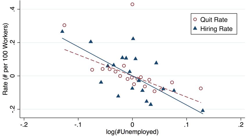
102                                  AER: INSIGHTS                          MARCH 2020

counterfactual time series of job openings and hires that shuts off procyclical
replacement hiring; job openings and hiring would be much smoother, falling by a
third less during recessions.
   We then formally study the aggregate effects of longer-lived jobs and replacement
hiring by introducing two parsimonious refinements into the textbook DMP model.
First, some employed workers quit, accepting outside job offers.
   Second, longer-lived jobs arise from a one-time, sunk job creation cost, not due
when firms repost old jobs. Hence vacancies, once created, command a strictly
positive equilibrium value, and firms optimally replacement-hire following quits.
Intuitively, job creation corresponds to constructing a new office from scratch;
replacement hiring is to fill an empty existing office. Zero job creation costs, imply-
ing zero value of vacancies and jobs as mere matches, nest the standard DMP model.
   A vacancy chain emerges: quitters leave behind valuable vacant jobs, which firms
repost, some of which are filled by employed job seekers, who in turn leave behind
their old jobs, and so forth. Vacancies beget vacancies.
   In equilibrium, replacement hiring and vacancy chains can raise employment by
boosting total job openings. This aggregate net effect depends on the crowd-out
response of new job creation, in our model guided by the adjustment cost parame-
ter for new job creation. We conduct a meta study of 15 empirical studies, finding
that such crowd-out appears very limited in the short run. For instance, temporary
hiring boosts due to targeted policy incentives do not crowd out hiring by ineligi-
ble employers (Cahuc, Carcillo, and Barbanchon 2019), and sharp labor demand
reductions by some employers do not lead other employers to expand in the short
run in the same local labor market (e.g., Mian and Sufi 2014, Gathmann, Helm, and
Schönberg 2018), even among tradables. Consequently, in the calibrated model,
quit-driven replacement hiring partially passes through into total job openings, and
ultimately into aggregate net employment.
   By accommodating equilibrium net effects, our model also overcomes Robert
Hall’s critique of the original fixed-jobs and pure-churn vacancy chains in Akerlof,
Rose, and Yellen (1988, p. 589): “ The explanation given for a vacancy chain […]
is defective because it does not recognize stochastic equilibrium. As long as the
unemployment rate is not changing over time, the chain does not end when someone
moves from unemployment to employment: that move has to be counterbalanced by
another move from employment to unemployment, which keeps the chain going.”
The aggregate net effects of our calibrated model are also consistent with the empir-
ical causal effect of job-to-job transitions on net employment levels established by
Shimer (2001) and Davis and Haltiwanger (2014) across US states, for which our
model’s vacancy chain mechanism therefore suggests a novel rationalization.
   The model additionally implies amplification of business cycles that stems from
the procyclicality of quits. In our model, recessions are times when fewer jobs open
up because incumbents stay put, cutting short the vacancy chain and reducing job
opportunities available to the unemployed, raising unemployment. In upswings, the
tightening labor market pulls employed workers out of their matches, and the vacan-
cies they leave behind add to the surge in vacancies, pushing down unemployment
further than without replacement hiring.
   We close by speculating that the trend decline in churn (Davis 2008, Davis
and Haltiwanger 2014, Moscarini and Postel-Vinay 2016, Mercan 2018) may, by
VOL. 2 NO. 1                 MERCAN AND SCHOEFER: JOBS AND MATCHES                  103

determining the strength of the vacancy chain, amplify labor market fluctu-
ations, consistent with the correlations in Galí and Van Rens (2017) for the
United States. Similarly, while worker flow rates in Germany—the context of our
vacancy survey— are comparable to many OECD countries (Elsby, Hobijn, and
Şahin 2013), replacement hiring may play an even larger role in higher-churn labor
markets such as the United States.

   Related      Literature.—Faberman        and     Nagypál     (2008)     investigate
establishment-level links between employment growth, quits, and job open-
ings, and build a micro model fitting cross-sectional establishment-level patterns.
Akerlof, Rose, and Yellen (1988) examine vacancy chains focusing on the match
quality improvements (amenities) with a fixed number of jobs (not studying equi-
librium). Lazear and Spletzer (2012) and Lazear and McCue (2017) study explicitly
“pure churn,” while our paper presents an equilibrium model and assesses poten-
tial net effects. Our paper is most closely related to Elsby, Michaels, and Ratner
(2019), who study vacancy chains in a rich model featuring on-the-job search and
large heterogeneous firms. Workers switch jobs to climb the productivity ladder.
Firms replacement-hire because of sticky employment-level targets, which the
authors support with establishment-level evidence on net employment persistence
despite turnover. Reicher (2011) investigates hiring chains with heterogeneous
firms and on-the-job search. Krause and Lubik (2006), Nagypál (2008), Menzio
and Shi (2011), Eeckhout and Lindenlaub (2018), and Moscarini and Postel-Vinay
(2018) present models featuring the labor supply channel, by which increased
on-the-job-search during upswings stimulates new job creation. Krause and Lubik
(2006) feature a mechanism akin to replacement hiring from a “bad” sector into
a “good” sector due to complementarities in final-goods production. Burgess and
Turon (2010) study on-the-job search and finite supply of job vacancies, but not
procyclical quits and recycled jobs. Fujita and Ramey (2007) introduce adjustment
costs in vacancies into a DMP model to generate empirically realistic hump-shaped
impulse responses of vacancies, but do not focus on reposting of vacancies or quits.
Coles and Moghaddasi-Kelishomi (2018) study layoffs and job destruction with
inelastic job creation, but do not feature quits and vacancy chains. Acharya and Wee
(2018) study the wage growth trend effects of an alternative notion of replacement
hiring by which employers search “on the job” for better workers.

                         I. Replacement Hiring in the Data

   (i) At the job level, surveyed employers classify the majority of job openings
as replacement hiring. (ii) An establishment-level event study estimates essentially
one new hire per quit. At the (iii) aggregate level, hiring and job opening time series
tightly track quits, and (iv) they might be much smoother in a no-replacement-hiring
counterfactual.

      A. Job-Level Evidence on Replacement Hiring from an Employer Survey

  A central contribution and motivation of the paper is our novel direct evidence
on the prevalence of old jobs and replacement hiring in total job openings. Our
104 AER: INSIGHTS MARCH 2020
source is a representative annual employer survey of 7,500 to 15,000 establishments
from 2000 to 2015 (German IAB Job Vacancy Survey). We exploit a variable on the
reason for the job opening, part of a section with details on the last filled job opening
in the last 12 months.
The bar chart in Figure 1, panel A, shows that 56 percent of job openings are
posted in response to quits.1 Of these, 47 percentage points (9 percentage points)
are permanent (temporary). Around 35 percent of vacancies target permanent net
job creation, and around 8 percent in response to temporary demand increases. The
composition is quite stable between 2000 and 2015 (online Appendix Figure A.1,
panel A).
B. Establishment-Level Effects of Quits on Hiring
At the establishment level, we estimate an almost one-to-one effect of quits
on replacement hiring. We use another annual representative establishment panel
survey (LIAB, from the German IAB), from 1993 to 2008, on annual cumulative
gross flows by type (quits, layoffs, hires), a “German JOLTS.” 2 We focus on hir-
ing outcomes since the point-in-time vacancy variable comes with temporal mis-
match, estimating an event study for establishment e’s year-t outcome for leads / lags
L ∈ {0, 1, 2, 3}:
{Hirese,t, Job Openingse,t} +L
Quitse,t+s
(1) ___________________ = β0 + ∑ νs _ + αe + αt + εe,t .
Empe,t−1 s= −L Empe,(t+s)−1
The variable νs measures the amount of (replacement) hires (or job openings) per
quit at event time s; αe (αt) are establishment (year) fixed effects.
Figure 1, panel B, plots the estimates (complemented by regression results in
online Appendix Tables A.1 and A.2).3 One incremental quit is associated with
between 0.74 and 1.0 additional hires ( p-value < 0.1 percent). Cumulating coeffi-
cients around t = 0 would imply even larger replacement hiring effects. The small
coefficients on the leads and lags confirm that replacement hiring occurs within the
year of the quit, making reverse causality (past hires triggering quits) unlikely.
Moreover, the binned scatter plots in online Appendix Figure A.1, panel B (C),
reveal a strikingly linear shape of the replacement hiring (job posting) relationship,
consistent with job-level replacement hiring, and motivating our model of atomistic
firm-jobs rather than multi-worker firms in Section II.4
1
The vacancy survey does not definitely distinguish quits from layoffs, but the connotation of examples given
(e.g., maternity leave is offered as an example cause for temporary replacement hiring, and later survey rounds
separate out retirement from permanent worker departures) suggests this quit interpretation.
2
We restrict our analysis to West Germany and establishments with at least 50 employees. We exclude extreme
observations (| d ln Empe,t | ≥ 40 percent employment growth and Quitse,t / Empe,t−1 ≥ 20 percent).
3
Online Appendix Table A.1, panel B, shows estimates for job openings consistent with the hiring effects if
annualized (multiplied by 12, supposing one-month vacancy duration), but noisier likely because job openings are
measured point-in-time.
4
Ancillary evidence by Isen (2013); Doran, Gelber, and Isen (2015); and Jäeger and Heining (2019) is consis-
tent with one-to-one replacement hiring.VOL. 2 NO. 1 MERCAN AND SCHOEFER: JOBS AND MATCHES 105
Panel A. Composition of job openings in Germany Panel B. Event study of hires following quits
60 1.4
3 leads/lags
1.2 2 leads/lags
50
Percent of vacancies
1 1 lead/lag
d hires/d quits
0.8 No leads/lags
40
0.6
Long-term 0.4
30 47.4%
Long-term 0.2
36.2%
20 0
−0.2
10 −0.4
Temporary 7.7% Temporary 8.7% −0.6
0 −3 −2 −1 0 1 2 3
New job creation Replacement hiring Year (leads/lags)
Panel C. US time series of job openings, hires, and quits
6
LTS JOLTS
5
Rate (per 100 employees)
4
3
2
1 Hires
Job openings
Quits
0
1959 1966 1974 1980 2001 2008 2015
Panel D. Cyclicality of job openings and quits Panel E. Cyclicality of new hires and quits
0.8 1
Deviation from trend (ppt)
Deviation from trend (ppt)
LTS JOLTS LTS JOLTS
0.6 0.8
0.6
0.4
0.4
0.2 0.2
0 0
−0.2
−0.2
−0.4
−0.4
−0.6
−0.6 Job openings
−0.8 Hires
Quits Quits
−0.8 −1
1959 1966 1974 1980 2001 2008 2015 1959 1966 1974 1980 2001 2008 2015
Figure 1. Replacement Hiring in the Data
Notes: Panel A: Composition of job openings (last filled job at establishment) by reason, 2000–2015 averages.
The temporary category includes seasonal factors. New job creation is phrased as a labor-demand increase
(“Mehrbedarf ”); replacement hiring is literal translation (“Ersatz”), where the temporary category includes
maternity leave and sickness. The survey excludes apprentices, “mini-jobs,” contract renewals or temp.-to-perm.
switches, temp workers, and subsidized (“1 euro”) jobs. Panel B: Establishment level event study of hires (per year)
on quits (per year). We plot 95 percent confidence bands for the 3-lag/lead specification, estimating regression
model (1), detailed in text. Panel C: Time series of quarterly averages of monthly data on job openings (point in
time), and hires (count per month), and quits (count per month), all as rates (per 100 employees). Panels D and E
plot detrended versions (HP-filtered with parameter 1,600).
Sources: IAB Job Vacancy Survey, IAB LIAB, BLS Labor Turnover Survey, and JOLTS.106 AER: INSIGHTS MARCH 2020
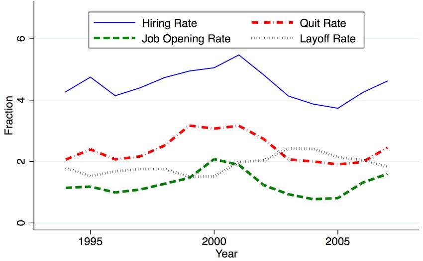
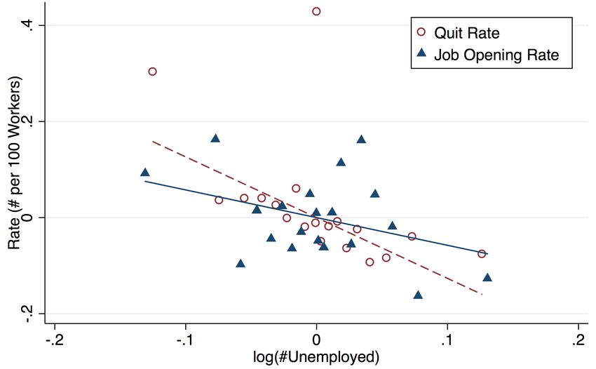
C. Time Series Comovement
Figure 1, panel C, plots the US time series of quits (count per month), job
openings (point in time) and new hires (count per month), averaged at the quar-
terly frequency. Figure 1, panels D and E, plot the detrended versions (HP-filtered,
smoothing parameter of 1,600).5 Aggregate quit rates are highly procyclical, and
comove around one to one with hiring and job vacancy rates. For example, during
the Great Recession, monthly quits per 100 workers fell from 2.5 to 1.5. Job open-
ings per 100 workers moved almost in lockstep, falling from 3.3 to 2, similarly
for monthly hires. The post-2000 data are from Job Turnover and Layoff Survey
(JOLTS) for the private sector; the earlier data are from the BLS Labor Turnover
Survey (LTS), which covers the manufacturing sector. Online Appendix Figure A.1,
panel D, confirms similar aggregate cyclical patterns for Germany; panel E ( F )
does so for quits and hires ( job openings) in response to regional business cycles
(municipalities).
D. Counterfactual Time Series without Replacement Hiring
Building on the previous empirical facts, we next present reduced-form counter-
factual time series that would arise absent replacement hiring fluctuations—i.e., if
reposted vacancies were stable, and only new job creation fluctuated. We will study
the equilibrium counterfactual in the cyclical analysis of the calibrated model in
Section IIID.
Total vacancies v = r + n consist of reposted old jobs r and new jobs n. Our
job-level evidence suggests a share of reposted vacancies ρ = r/(r + n) = 0.56 in
Germany. Percent deviations from trend in total vacancies are a ρ-weighted average
of those in r and n:
(2) _ dr + (1 − ρ)_
dv = ρ _ dn ,
v r n
where in practice we study deviations from an HP trend with quarterly log time
series (smoothing parameter of 1,600).
The object of interest is the counterfactual vacancy time series that would
mechanically emerge if dr = 0 at all points while n’s path remained unaffected.
We back out new job creation as total-vacancy growth net of growth in repostings
by rearranging identity (2), then proxying for reposted vacancies with worker quits
(exploiting the one-to-one, linear replacement hiring estimated in Section IB):
(3)
˜
_
dv
v |
dr = 0
= (1 − ρ)_
dn = _
n
dv − ρ _
v
dr ≈ _
r v
dQuits
dv − ρ _
Quits
.
Figure 2, panel A, presents this counterfactual vacancy series along with the
empirical one, relying on JOLTS quit and vacancy data from 2000 through 2018. The
graph reveals amplification potential: during the Great Recession, total job openings
5
We have found similar results with the detrending procedure advocated by Hamilton (2018), with overall
larger, yet proportional, amplitudes.VOL. 2 NO. 1 MERCAN AND SCHOEFER: JOBS AND MATCHES 107
Panel A. Counterfactual job openings Panel B. Counterfactual hires
30 15
Deviation from trend (%)
Deviation from trend (%)
20 10
10 5
0 0
−10 −5
−20 −10
−30 −15
−40 −20
01 02 03 04 05 06 07 08 09 10 11 12 13 14 15 16 17 01 02 03 04 05 06 07 08 09 10 11 12 13 14 15 16 17
Counterfactual—ρ = 0.56 Job openings (JOLTS) Counterfactual—ρ = 0.56 Hires (JOLTS)
Counterfactual—ρ = 0.927 Counterfactual—ρ = 0.927
Panel C. Counterfactual job openings—HWI
30
Deviation from trend (%)
20
10
0
−10
−20
−30
−40
52 57 62 67 72 77 82 87 92 97 02 07 12 17
Counterfactual—ρ = 0.56 Job openings (HWI)
Counterfactual—ρ = 0.927
Panel D. Cyclicality of (UE) job finding and quit rates
20
Deviation from trend (%)
15
10
5
0
−5
−10
−15 UE (CPS)
−20 Quits (JOLTS)
−25
01 02 03 04 05 06 07 08 09 10 11 12 13 14 15 16 17
Figure 2. Counterfactual Time Series and Quit Cyclicality
Notes: All time series are quarterly, logged and HP-filtered with smoothing parameter λ = 1,600. Consistent with
the decomposition exercise, they are in levels (counts), rather than rates (per 100 workers). The monthly time series
(JOLTS, CPS) have been averaged at the quarterly frequency. Panel A: Actual and counterfactual job openings
from JOLTS. Panel B: Actual and counterfactual hires from JOLTS. Panel C: Actual and counterfactual job openings
from the Help Wanted Index. Panel D: Cyclical component of UE job finding rates (CPS, our construction) and quit
rates (JOLTS, count of quits per month per 100 employees). A regression reveals a linear coefficient of UE on quit
rates of 0.985 ( R 2 = 0.77 ).
would have only dropped by 20 percent instead of 30 percent. Panel B illustrates
the smoothing predicted for hires. Panel C extends the vacancy time series to 1951108 AER: INSIGHTS MARCH 2020
using the Help Wanted Index (Barnichon 2010), confirming the role of replacement
hiring in all post-War recessions.6
The Role of Churn ρ .—The amplification potential naturally depends
on ρ, the share of reposted vacancies in total vacancies. Our baseline calibration
to ρ = 0.56, from the German context, is likely a lower bound for higher-churn
economies such as the United States. A back of the envelope extrapolation suggests
a US ballpark ρ US ≈ 0.93 .7 Figure 2 panels A– C also plot this more speculative
counterfactual, illustrating the potential range of amplification.
II. A Model of Jobs, Matches, and Replacement Hiring
We introduce longer-lived jobs, a distinction between jobs and matches, and
replacement hiring into the DMP model, and then study their equilibrium conse-
quences quantitatively in Section III.
Preview.—We add a one-time, sunk cost per new job created, k(nt),
with k′(nt) ≥ 0, where nt denotes the number of new, initially vacant, jobs. The net
value of a newly created job, Nt, is the value of a vacant job Vt minus upfront cost
k (nt): Nt = Vt − k (nt). Free entry for new job creation pushes equilibrium Nt
to zero, and hence if k (0) > 0, the equilibrium value of a vacant job is strictly
positive:
(4) Vt = k (nt).
Here, when a worker-firm match dissolves that leaves the job intact, the firm
optimally reposts the valuable vacancy—i.e., engages in replacement hiring. Jobs
outlive matches.
Such longer-lived jobs render the vacancy stock vt predetermined, following law
of motion:
(5) vt = nt + (1 − qt−1) vt−1 + rt ,
where q and r denote the vacancy filling rate and newly reposted vacancies,
respectively.
A vacancy chain emerges: vacancies can meet employed workers, who quit to
switch jobs, leaving their jobs vacant, which firms optimally repost, and so forth.
Vacancies beget vacancies.
6
To extrapolate the quit time series to the pre-JOLTS time period, we estimate an “Okun’s law” for quits.
Specifically, we regress the quarterly JOLTS detrended log quit level on the detrended unemployment rate
(R 2 = 0.88). We then project that estimated semi-elasticity (− 0.1) onto the full unemployment time series.
7
Online Appendix Figure A.1, panel D, highlights that German churn is an order of magnitude below the US
ones (since it represents annual hires while JOLTS is monthly), consistent with cross-country evidence on worker
flows (Elsby, Hobijn, and Şahin 2013). Let ρ i = r i/(r i + n i) denote the share of repostings in total job openings
for country i. Under the approximation of one-to-one quit-replacement hiring, ρ can be stated in terms of quit
rate Q i and new job creation rate C i: ρ i = Q i/(Q i + C i) , such that C i = Q i[1 / ρ i − 1]. Under the perhaps extreme
assumption C i = C j = C, we can express: ρ j = Q j/(Q j + C) = Q j/(Q j + Q i[1 / ρ i − 1]) = 1/(1 + Q i / Q j
[1 / ρ − 1]). For the United States and Germany, Q / Q ≈ 10, and then ρ = 0.56 implies ρ = 0.9272.
i US DE DE USVOL. 2 NO. 1 MERCAN AND SCHOEFER: JOBS AND MATCHES 109
This vacancy chain can have aggregate net effects beyond churn, on total
vacancies—depending on the response by new jobs:
∈ [0, 1]
dvt
_ dnt
_
(6) = + 1.
∈[⏟
drt drt
−1, 0]
In our model, this “crowd-out” dnt /drt is guided by the shape of job creation cost
k (nt). Since empirical crowd-out—we show in Section IIIC—appears small in the
short run, replacement hiring passes through into total job openings, some of which
are filled by the unemployed, hence raising aggregate net employment.
A. Environment
Time is discrete. There is a unit mass of workers, with risk neutral preferences
and discount factor β, who are either employed or unemployed. There is a larger
mass of potential firm entrants. Firms are single-worker jobs, owned by workers.
Jobs, Matches, Separations, and Vacancies.—Jobs denote long-lasting entities
that can be vacant or matched. Matches denote a job that is filled by a particular
worker. In each period, jobs are exogenously destroyed with probability δ: the
worker becomes unemployed, the job disappears forever without replacement hiring.
Matches moreover dissolve with probability σ (the worker becomes unemployed),
or through a worker job-to-job transition (described below). These jobs—vacated by
what we label “quits” going forward—remain intact with probability γ and trigger
replacement hiring (while (1 − γ) of match dissolutions destroy the job).
Job Creation.—One new job (aggregate count n) can be created at sunk
cost k(n). Note, k(n) = 0 nests standard DMP.8 If k(n) > 0, firms will repost jobs
vacated by quits. All vacancies also require the standard per-period maintenance
cost κ.
Matching.—Both unemployed and employed workers look for jobs.
Employed workers search with intensity λ relative to unemployed workers.
Meetings between vacancies and workers follow a constant returns match-
ing function M(s, v) < min {s, v}. Labor market tightness θ = v/s
is the ratio of vacancies v to searchers s = u + λe. The job [worker]
finding probability for an unemployed (employed) worker [vacancy] is
f (θ) = M/s = M(1, θ) (λ f (θ)) [q(θ) = M/v = M(1 / θ, 1)].
Timing.—The timing of events within period t is:
(i) st, the state of the economy, is realized, including unemployment ut and
beginning-of-period (inherited) vacancies ṽt.9
8
Fujita and Ramey (2007) use a similar cost to smooth out vacancy responses in a model without replacement
hiring.
9
Our experiments will comprise perfect foresight transition dynamics, so we do not make st explicit here.110 AER: INSIGHTS MARCH 2020
(ii) Employed workers consume a bargained wage wt and produce yt,
unemployed workers receive unemployment benefit b.
(iii) Firms create nt new jobs at cost k(nt) each, and pay flow cost κ per
vacancy. This determines total vacancies vt = ṽt + nt and market tightness
θt = vt/(ut + λ (1 − ut)).
(iv) f (θt) ut of unemployed workers find jobs, λ f (θt) et of employed workers
switch jobs.
(v) Fraction δ of jobs are exogenously destroyed; these workers become
unemployed.
(vi) Fraction σ of matches are exogenously dissolved; these workers become
unemployed. Share γ (1 − γ) of jobs hit by EE quits or σ shocks can be
reposted as vacancies (are destroyed).
The law of motion for unemployment is
(7) ut = (1 − (1 − δ )(1 − σ) f (θt−1)) ut−1 + δ
(1
− ut−1) + − δ )σ(1 − ut−1).
(1
stay unemployed EU: job destruction EU: match separation
Due to sunk cost k(n), the vacancy stock is predetermined, with law of motion:
(8)
⎛ ⎞
⎜ ⎟
= γ(σ+(1−σ)λ f (θt−1))et−1
+ (1 − δ ) (1 − (1 − σ)q(θt−1))vt−1 + γ (θt−1) et−1 +
σ(1 − λ f (θt−1))et−1 . .
( )⎠
vt = nt λ f
⏟
new
⎝
unfilled reposted: EE
reposted: EU
beginning-of-period (inherited) vacancies ṽt
Below, we drop time subscripts and use primes (′ ) to denote the next period.
B. Value Functions
Value functions are expressed recursively, after the aggregate state is realized
(i.e., after subperiod i).
Worker Problem.—The worker when unemployed consumes unemployment
benefit b. She may match with a job, to start work next period (unless a match/job
shock hits), or stays unemployed:
(9) U(s) = b + β(1 − δ )(1 − σ) f (θ)E[W(s′ )]
+ β (1 − (1 − δ )(1 − σ) f (θ))E[U(s′ )].VOL. 2 NO. 1 MERCAN AND SCHOEFER: JOBS AND MATCHES 111
An employed worker consumes wage w(s), and then may stay, quit to another job,
or become unemployed:
(10) W(s) = w(s) + β(δ + (1 − δ )σ)E[U(s′ )]
⏞
+ β(1 − δ )(1 − σ) (1 − λ f (θ) + λ f (θ)) E[W(s′ )].
stay
quit
=1
Maximally Parsimonious On-the-Job Search.—We present a parsimonious
version of job-to-job quits because its hard-wired unit-elasticity between job-to-job
quit (λ f (θ)) and unemployed job finding (UE, f (θ)) turns out to produce empirically
realistic quits, as shown in panel D of Figure 2, where we plot log deviations from
trend of the quarterly quit rate (based on the JOLTS) against the job finding rate
(based on the CPS) of the unemployed (regression coefficient of UE on quit rates of
0.985, R 2 = 0.77).10
Online Appendix E presents a richer model that explicitly rationalizes job switch-
ing with heterogeneity in match quality, and features endogenous job search effort—
with similar amplification results.
Firm Problem.—Newly created jobs have value
(11) N(s) = − k(n) + V(s).
Once created, a vacancy carries value
(12) V(s) = − κ + β(1 − δ )[q(θ)(1 − σ)E[J(s′ )] + (1 − q(θ)(1 − σ))E[V(s′ )]].
A vacancy incurs flow cost κ and matches with a worker with probability q(θ); oth-
erwise it stays vacant or is destroyed.
A filled job produces output y and pays wage w. If the match separates (σ shock
or job-to-job quit), the job enters next period as a vacancy with probability γ (and
otherwise becomes destroyed and is worth 0), hence its value is:
(13) J(s) = y − w(s)
+ β(1 − δ)[γ(σ + (1 − σ)λ f (θ))E[V(s′ )] + (1 − σ)(1 − λ f (θ))E[ J(s′ )]].
Free Entry.—Free entry in job creation drives new job values
N(s) = − k(n) + V(s) to zero:
(14) V(s) = k(n).
10
CPS job-to-job transition measures (with short/no nonemployment spell) are slightly smoother than quits but
include layoffs/job destruction, not exclusively quits.112 AER: INSIGHTS MARCH 2020
C. Match Surplus and Wage Bargaining
The worker’s outside option is unemployment, even for a job switcher, who must
renounce her old job before bargaining with the new employer (rather than permit-
ting sequential bargaining as in Postel-Vinay and Robin 2002; our simplification is
also used in Fujita and Ramey 2012). Joint match surplus S(s) is
(15) S(s) = J(s) − V(s) + W(s) − U(s).
Wages are determined according to generalized Nash Bargaining with worker
share ϕ ∈ (0, 1) to maximize
(W(s) − U(s)) (J(s) − V(s))
ϕ 1−ϕ
(16) ,
implying linear surplus sharing, worker (firm) capturing share ϕ (1 − ϕ) of joint
surplus S:11
(18) ϕS(s) = W(s) − U(s),
(19) (1 − ϕ)S(s) = J(s) − V(s).
D. Stationary Equilibrium Definition
We solve the model in steady state. The stationary equilibrium of the model is
a set of value functions W(s), U(s), J(s), and V(s), wage function w, and new job
creation n such that: (i) Worker and firm values satisfy Bellman Equations (9), (10),
(12), and (13). (ii) Wage w maximizes equation (16). (iii) Unemployment u and
vacancies v follow the laws of motion (7) and (8). (iv) New job creation n satisfies
free entry condition (14).
E. Calibration
Panel A of online Appendix Table B.1 summarizes the calibration; Panel B
reports the targeted moments and the model fit. We discuss below, formally
and informally, how these target moments help identify the model parameters.
Computational details are in online Appendix B. We relegate the specification and
calibration of job creation cost k (n) to Section III.
11
Using (9), (10), (12), (13), (15), (18), and (19), joint surplus is
(17) S(s) = y − b + κ + β (1 − δ )(1 − σ)[1 − λ f (θ) − f (θ)(1 − λ)ϕ − q (θ)(1 − ϕ)]E[S(s′)]
+ β (1 − δ )[(1 − σ)(1 − λ f (θ)) + γ σ − 1 + γ (1 − σ)λ f (θ)]E[V(s′)],
where V(s) = − κ + β (1 − δ )[q(θ)(1 − σ)(1 − ϕ)E[S(s′ )] + E[V(s′ )]].VOL. 2 NO. 1 MERCAN AND SCHOEFER: JOBS AND MATCHES 113
We start with standard DMP parameters set outside of the model. Our
model period is a month. Discount factor β = 0.9967 targets an annual
interest rate of 4 percent. Standard Cobb-Douglas matching function
M(s, v) = 4s η v 1−η features elasticity of matches with respect to total search
effort η and matching efficiency 4. Unemployed (employed) job finding [vacancy
filling] rate is f (θ) = 4θ 1−η (λ f (θ) = λ4 θ 1−η) [q(θ) = 4 θ −η]. We set η = 0.5,
as standard. Inconsequential for our study of relative amplification, we set ϕ = 0.5
(Hosios condition) and pragmatically b = 0.9 following Fujita and Ramey (2007),
who in turn follow Hagedorn and Manovskii (2008) for sizable amplification.
GMM sets the remaining DMP parameters. Targeting a monthly
UE rate of 45 percent (Shimer 2005) with model counterpart
(1 − δ)(1 − σ) f (θ) = (1 − δ )(1 − σ)4 θ 1−η, yields 4 = 0.6542. Steady-state
unemployment rate EU/(EU + UE) = 5.7 percent disciplines EU rate
δ + (1 − δ)σ = 2.72 percent. Targeting job filling rate (1 − δ)(1 − σ)q(θ) = 0.9
(Fujita and Ramey 2007) normalizes steady-state market tightness
((1 − δ)(1 − σ) f (θ))/((1 − δ)(1 − σ)q(θ)) = θ = 0.45/0.9 = 0.5. We then
find a vacancy posting cost κ = 0.1611 consistent with free entry and this tight-
ness, given job creation costs k(n), discussed below. We pin down on-the-job
search efficiency λ = EE/UE = 0.056, targeting an average monthly quit rate
of 2.5 percent (CPS EE, Fujita and Nakajima 2016, and JOLTS quit rate). To sep-
arately identify match-separation σ = 0.0051 and job-destruction δ = 0.0222
γ (1 − δ )[λ f + σ (1 − λ f )]e
rates, we target a vacancy reposting share ρ = _________________ = 56
n + γ (1 − δ)[λ f + σ (1 − λ f )]e
percent (see Section IA).
III. Aggregate Effects of Replacement Hiring and Vacancy Chains
Job Creation Cost k(n).—We organize our discussion of the aggregate
implications of replacement hiring and vacancy chains around job creation cost
k(n), specifying it in terms of deviations from steady-state n–:
(20) n − n.
k(n) = k1 + k2 × _____
–
n–
The variable k1 guides (micro) replacement hiring by generating positively valued
vacancies, which we discuss and calibrate first below. We then move to equilibrium
aggregate consequences of replacement hiring by calibrating k2, the degree to which
hiring costs are increasing in n, e.g., due to adjustment costs.
A. Firm-Level Replacement Hiring
Free entry (14) implies that firms create vacancies until the “k(n)-profit” condition
(replacing the standard DMP zero-profit) is satisfied in all periods:
κ + (1 − β(1 − δ )) k1 + (1 − β (1 − δ )E[_____
n − n– ]) n–
(21) n′ − n _____
n − nk
– –
2
= β(1 − δ )q(θ)(1 − ϕ)E[S(s′ )].114 AER: INSIGHTS MARCH 2020
Parameter k1 > 0 ensures a positive ex post value of vacancy in steady state. As a
result, jobs vacated by quits are reposted. We set k1 to 0.1, large enough to ensure
that k(n) > 0 and thus n > 0 in all our subsequent experiments. Equilibrium entry
condition (21) clarifies that κ and k1 affect steady-state surplus similarly, and we
let κ = 0.1611 be estimated to target normalized θ = 1 / 2. We also set γ = 1 to
match the ∼ 1.0 (cumulative) estimate from Section IB.
B. Vacancy Chains
Our model features a vacancy chain, by which vacancies beget vacancies
through quits and the associated replacement hiring. Formally, the chain tracks a
single vacancy and all the additional vacancies it triggers by meeting employed
workers (probability 1 − ϒ), who quit and leave behind another vacancy, which
we then track, and so forth. The chain ends when it meets an unemployed searcher
(probability ϒ = u/(u + λ (1 − u))), or is destroyed by a δ -shock. The chain
length C counts these vacancies, obtained recursively:12
(23) E[C ] = 1 ⋅ [δ + (1 − δ )qϒ] + (1 − δ )q(1 − ϒ)(E[C ] + γ)
+ (1 − δ )(1 − q)E[C ]
δ + (1 − δ)q(ϒ + γ (1 − ϒ))
= ____________________.
1 − (1 − δ)(1 − qϒ)
In our calibrated model, this length is 1.88, i.e., one vacancy entails 0.88 vacancies
in excess of itself.
C. Aggregate Equilibrium Effects
The vacancy chain is a microeconomic concept tracking the life cycle of a
single vacancy and its “offspring.” To study the equilibrium implications of the
vacancy chain, we consider a one-time exogenous addition to the stock of inherited
vacancies.13 Whether and how much such a vacancy “injection” actually adds to the
total stock on net (and then affects other quantities) depends on the response in new
job creation.
Crowd-Out by New Job Creation: Model.—The key response to a vacancy
injection—and in fact the only contemporaneous one in the vacancy law of
motion—stems from the crowd-out response by new job creation. In terms of
If δ = 0 and γ = 1, E[ C ] = (0.057 + 0.0556 × (1 − 0.057))/0.057 = 1.92 ≈ 1.88 since δ ≪ ϒ.
12
Alternatively, the length can be calculated as a binomial sum of iso-length paths:
(δ + (1 − δ )qϒ)(γ (1 − δ )q(1 − ϒ)) c−1
c= 1 t= c−1 ( ((1 − δ )(1 − q) + (1 − δ )q (1 − ϒ)(1 − γ)) (c−1)−t )
∞ ∞ ∞
(22) E[C ] = ∑ c · Pr (C = c) = ∑ c ∑
( )
t _________________________________________ .
c= 1 t − (c − 1)
13
This ad hoc experiment may capture, e.g., cyclical shifts in public employment or sectoral shocks.VOL. 2 NO. 1 MERCAN AND SCHOEFER: JOBS AND MATCHES 115
beginning-of-period vacancy shifts dṽ, one additional vacancy is crowded out
by dn/dṽ ∈ [− 1, 0], and on net raise the vacancy stock only by (1 + dn/d ṽ ) ≤ 1.
Crowd-out d nt/d ṽt is an equilibrium outcome and depends on k2, the increasing
degree of hiring cost. In panel A of Figure 3 we plot d nt/d ṽt for various values
of k2, along with total-vacancy response d vt/d ṽt = 1 − d nt/d ṽt , where d x = xt −
x– denotes level deviation from steady state. The simulated data plots the first-period
(hence largest) response to a (beginning-of-period) “vacancy injection” εvt ̃ shock:14
(24) vt = nt + (1 − δ)((1 − (1 − σ)q(θt−1)) vt−1
+ γ(σ + (1 − σ)λ f (θt−1)) et−1) + εvt ̃ .
In calculating the underlying impulse responses, we focus on perfect foresight
transition dynamics following one-time, unanticipated shocks out of steady state,
using a shooting algorithm (details in online Appendix B.3). We plot and discuss the
full impulse response functions (IRFs) for new job creation (and unemployment and
vacancies) in online Appendix C.
The case of k2 = 0 provides an extreme benchmark of perfect neutrality of vacancy
inflows such as from replacement hiring: full crowd-out (dn/dṽ = − 1) and no
pass-through into total vacancies (d v/d ṽ = 0), since n adjusts such that v ⁎ = θ ⁎ ⋅ u,
and θ remains—as in the standard DMP model—the equilibrating variable.
Reposting then merely tilts the composition from new to old jobs in the economy,
despite longer-lived jobs and reposting.
By contrast, for all k2 > 0, replacement hiring has net effects on aggregate
labor market outcomes. Intuitively, at the original n–, a vacancy injection incipiently
lowers V a lot (as q falls and w increases due to higher θ), beyond the original
free entry consistent k(n). Free entry leads n to fall, the process that drives the
adjustment to the new equilibrium by again raising V and, due to k2 > 0, also
lowering k(n). The incidence between k(n) and V—whether new jobs fully restore
the original total-vacancy level, and V and k(n) to the original levels—depends on
the shape of k(n). When k′(n) > 0 (k2 > 0), the fall in new job creation stops
“prematurely,” at a lower equilibrium k(n) = V, hence implying higher total job
openings. Under k2 > 0 (k2 → ∞), repostings are offset less than one to one
(not at all) and thus pass through (completely) into total job openings and aggregate
employment.
Empirical Evidence for Crowd-Out, and Calibration of k2.—We calibrate k2
by matching the model crowd-out to empirical targets. In Figure 3, panel B, we
conduct a meta study and convert 15 suitable empirical studies into implied
crowd-out measures. Strikingly, nearly every study points toward zero (if not
positive) short-run crowd-out. For example, subsidies boosting hiring among eli-
gible firms do not curb hiring by ineligible employers in the same labor market
(Cahuc, Carcillo, and Barbanchon 2019), and sharp hiring (employment) reductions
14
The shock hits in period t = 1 (beginning of period), and is zero for all t ≠ 1. We consider a shock small
enough, specifically 1 percent of steady-state vacancy stock, to not crowd out n1 below zero, although we have
checked that crowd-out is quite stable in shock size.116 AER: INSIGHTS MARCH 2020
Panel A. Model: Crowd-out of vacancy inflow by new jobs
1 120
0.8
100
0.6
0.4
Our calibration 80
0.2
Percent
0 60
−0.2
Standard DMP
40
−0.4
−0.6 dn/ε1v
20
dv/εv1
−0.8 Relative amplification
−1 0
0 1 2 3 4 5
k2
Panel B. Empirical meta study: Short-run employment crowd-out
Full crowd-out No crowd-out
Standard DMP (k2 = 0) (k2 = ∞)
de Blasio and Menon (2011)
Jofre-Monseny, Sánchez-Vidal, and Viladecans-Marsal (2018)
Giupponi and Landais (2018)
Marchand (2012)
Acemoglu et al. (2016)
Black, McKinnish, and Sanders (2005)
Cahuc, Carcillo, and Le Barbanchon (2019, jobs)
Zou (2018)
Cahuc, Carcillo, and Le Barbanchon (2019, firms)
Mian and Sufi (2014)
Moretti (2010)
Jofre-Monseny, Silva, and Vázquez-Grenno (forthcoming)
Cerqua and Pellegrini (2018)
Gathmann, Helm, and Schönberg (2018)
Weinstein (2018)
Moretti and Thulin (2013)
−1.5 −1 −0.5 0 0.5 1 1.5
dEmpSpillover/dEmpDirect
Figure 3. Short-Run Employment Crowd-Out in the Model and the Data
Notes: Panel A presents simulated model responses of new job creation n and total vacancy stock v upon impact
to an exogenous injection of vacancies as a function of the vacancy cost creation parameter k2. The right y-axis
plots the corresponding relative amplification of the baseline model compared to a no-reposting counterfac-
tual, in response to a productivity shock, described in Section IIID. Panel B presents a meta study of empiri-
cal estimates speaking to employment crowd-out underlying our calibration of k2. We describe the papers and
detail our calculations of the spillover effects in online Appendix D. Some sensitivities are backed out from
elasticities. Most studies report crowd-out effects with SEs. For the others, we either replicate results (Mian
and Sufi 2014, Acemoglu et al. 2016) and estimate crowd-out SEs in an IV strategy to estimate crowd-out as
the ratio of spillover to direct effects β Spillover/β Direct for some instrument affecting a subset of employ-
ers, and report SEs of the IV effect. In cases where we cannot access the data directly to reestimate IV SEs
(Gathmann et al. 2018; Cahuc, Carcillo, and Barbanchon 2019; Weinstein 2018; Giupponi and Landais 2018),
method as follows (i.e., be forced to assume
we could construct SEs with the Delta_____________________ a zero covariance term):
_________
SE (β S( pillover) / β D(irect)) = SE D / β S ⋅ √1 + (β S / β D) 2 ⋅ (SE S / SE D) 2 = SE D / β S ⋅ √1 + ( t S / t D ) 2 . In practice,
since spillover effects are small compared to direct effects, and since direct effects are precisely estimated, these
SEs are close to SE Direct / β Spillover, which we therefore report for this subset.VOL. 2 NO. 1 MERCAN AND SCHOEFER: JOBS AND MATCHES 117
do not lead unaffected employers in the same local labor market to expand in the
short run even within the tradable sector (e.g., Mian and Sufi 2014, Gathmann et al.
2018). Some caveats apply to our extrapolation from local to aggregate crowd-out.15
Based on the preponderance of the evidence, we set k2 = 1, still implying some
crowd-out, d nt/d ṽ = − 0.1183.
Equilibrium Effects of Reposting: The Vacancy Multiplier.—To investigate the
dynamic equilibrium effects of a (one-time, perfectly transitory) vacancy injection ε ṽ
such as arising from reposting, we define a vacancy multiplier, which cumulates the
vacancy infl ows generated by the shock (as deviations from steady-state v– infl ow) over
horizon h,
∑hs= 1 (v infl ow
− v– infl ow)
(25) M(h) = _______________
s
,
ε v1̃
where v infl
s
ow
= ns + (1 − δ)γ (σ + (1 − σ)λ f (θs−1)) es−1 + ε vs ̃ captures the total
inflow of newly created and reposted vacancies (with ε vs ̃ = 0 ∀ s ≠ 1).
In addition, we decompose the multiplier. First, we plot the “one-only” multi-
plier that would arise if only one of the variables shifted (the rest held at steady
state). Second, we plot the “all-but-one” complementary multiplier: if all variables
adjusted except for the variable of interest kept at its steady state.
Figure 4, panel C (impulse response in companion panel A), reveals that the
equilibrium multiplier reaches around 1.37. The immediate vacancy pass-through
in period one is 0.88 = 1 + dn/d ṽ , and after 3 (6) [12] months the multiplier has
reached 1.03 (1.16) [1.29]. The first implication is the positive level: rather than
being crowded out as in the standard DMP model, an exogenous vacancy injec-
tion raises the aggregate vacancy stock. This result motivates our discussion of
business-cycle amplification in Section IIID below.
Second, the multiplier exceeds 1.00, implying that the model features amplifi-
cation akin to the micro vacancy chain: a given vacancy injected into the econ-
omy “generates” an additional 0.37 vacancies in excess of itself. The “one-only”
decompositions in panel C clarify that much of the multiplier is due to the job
finding boost—the equilibrium analogue of the micro vacancy chain. Still, at 1.37
the equilibrium multiplier remains below the micro vacancy chain (1.88), confirm-
ing the importance of the equilibrium perspective. Here, the “all-but-one” decom-
position panel D (IRFs in B) clarifies that crowd-out by new job creation is the
culprit: if n were held at steady state, the multiplier would reach around 2.25, even
exceeding the micro vacancy chain (1.88). Hence our limited crowd-out calibration
of k2 leaves new job creation with a quantitatively important role.
15
First, most studies do not differentiate between employment and hiring (although Cahuc, Carcillo, and
Barbanchon 2019 do and find similar estimates (Table 3)). Second, we do not rescale the spillover-treated (e.g.,
tradable) sector to the full labor market (e.g., by 1 / Share Tradable), which would further increase the positive
estimates. Third, agglomeration forces may mask crowd-out (Moretti 2010, Gathmann et al. 2018). Fourth,
non-local other (e.g., capital) markets may imply larger crowd-out for national experiments. Fifth, mismeasured
labor market overlaps may bias crowd-out away from − 1, although matching functions appear consistent across
levels of aggregation (Petrongolo and Pissarides 2001). Moreover, e.g., Gathmann et al. (2018) show robustness to
year-industry-location cells.118 AER: INSIGHTS MARCH 2020
Panel A. One-only decomposition Panel B. All-but-one decomposition
0.15 Only job creation n 0.15 Constant job creation n
Only contact rate f Constant contact rate f
Impulse response
0.1 Only employment e 0.1 Constant employment e
Total effect Total effect
0.05 0.05
0 0
−0.05 −0.05
−0.1 −0.1
5 10 15 20 25 30 35 40 5 10 15 20 25 30 35 40
Panel C. One-only decomposition Panel D. All-but-one decomposition
2.5 2.5
Only job creation n Only employment e
2 Only contact rate f Total effect 2
Vacancy multiplier
1.5 1.5
1 1
0.5 0.5
0 0
Constant job creation n Constant employment e
−0.5 −0.5 Constant contact rate f Total effect
−1 −1
5 10 15 20 25 30 35 40 5 10 15 20 25 30 35 40
Figure 4. Decomposing the Vacancy Multiplier
Notes: The figure presents impulse responses (panels A and B) and cumulative vacancy multipliers (panels
C and D) of vacancy inflows in response to a perfectly transitory exogenous increase in the vacancy stock by
1 percent, for simulated time series and its components. The variables are normalized by the size of vacancy injec-
tion ε v1̃ , which is not plotted. Panels A and C additionally present “one-only” inflows (that only permit one variable
to move from steady state); panels B and D present “all-but-one” inflows (that keep only one variable at steady
state). The total effect is (nt + (1 − δ ) γ (σ + (1 − σ)λ ft−1 )et−1 + ε v1 − v– Infl ow) / ε v1̃ . We then decompose this total
–
effect. The one-only decomposition features (i) the only job creation n effect (nt − n– )/ ε v1̃ ; (ii) the only contact rate
f effect (1 − δ ) γ (1 − σ)λ( ft−1 − f )e– / ε v1̃ ; (iii) the only employment e term, where we plot the sum of (iiia) the
–
mechanical employment rate effect (1 − δ ) γ (1 − σ)λ f (et−1 − e–) / ε 1ṽ , (iiib) the small effect of the employment
–
change on quits through σ shocks (1 − δ )γσ(et−1 − e ) / ε v1̃ , as well as (iiic) the small interaction between the two
–
(1 − δ )γ (1 − σ)λ ( ft−1 − f )(et−1 − e–) / ε v1̃ .
–
Online Appendix Figure F.1 illustrates the larger multiplier in an economy with
lower crowd-out of 5.95 percent (rather than 11.83 percent, using k2 = 3.1).
D. Business Cycle Implications
We close with a natural application: amplification of business cycle shocks stem-
ming from the dramatic procyclicality of quits and hence of replacement hiring, as
foreshadowed in the empirical counterfactual in Section ID.
Figure 5 presents the impulse responses from three experiments. To isolate the
incremental amplification from the vacancy multiplier, we juxtapose our model
(green solid lines) with two benchmarks that deactivate it, but otherwise feature theVOL. 2 NO. 1 MERCAN AND SCHOEFER: JOBS AND MATCHES 119
New job creation Vacancy stock Unemployment
8 8 0
7 7 −0.5
6 6 −1
5 5 −1.5
−2
y shock
4 4
3 −2.5
3
2 −3
1 2 −3.5
0 1 −4
−1 0 −4.5
0 20 40 60 80 100 0 20 40 60 80 100 0 20 40 60 80 100
0.8 0.45 0.25
0.6 0.4
0.35 0.2
0.4 0.3 0.15
λ shock
0.2 0.25
0.2 0.1
0
0.15
−0.2 0.1
0.05
−0.4 0.05 0
0
−0.6 −0.05 −0.05
0 20 40 60 80 100 0 20 40 60 80 100 0 20 40 60 80 100
0.8 0.4 0
0.6 0.2 −0.1
0.4 −0.2
0 −0.3
# shock
0.2
−0.2 −0.4
0
−0.4 −0.5
−0.2
−0.6
−0.4 −0.6
−0.7
−0.6 −0.8 −0.8
0 20 40 60 80 100 0 20 40 60 80 100 0 20 40 60 80 100
Reposting No reposting Full crowd-out, k(vInflow)
Figure 5. Impulse Responses: The Role of Reposting and Limited Crowd-Out
Notes: Impulse response functions of new job creation, vacancy stock and unemployment to aggregate productivity,
on-the-job search intensity and matching efficiency shocks. y-axes measure percent deviations from steady
state. The graphs arise from three model variants: the baseline model with reposting and imperfect crowd-out
(green solid line), the no-incremental-reposting economy (blue dashed, where repostings are held at steady state
yet the job creation cost mirrors the baseline model), and the full-crowd-out economy (red dash-dotted, where job
creation costs depend on total inflows rather than new job creation, yet there is reposting).
same steady state and adjustment costs. (While k2 = 0 would generate neutrality,
it would also shut off adjustment cost k ′(n), independently generating amplification.
While γ = 0 would shut off reposting, it would also change steady-state flows,
surplus and the discounting of the shock process.)
First, in the “no (incremental) reposting economy” (blue dashed lines), we
artificially hold acyclical (at steady state) any fluctuations in reposting infl ows
in the vacancy law of motion.16 Second, we add a “ full crowd-out economy”
(red dash-dotted lines), where vacancy creation costs k (·) depend on total vacancy
16
Here perhaps an unmodelled actor neutralizes reposting fluctuations by adding and subtracting to ṽt (but not
to nt) to obtain: vt = nt + (1 − δ )((1 − (1 − σ)q(θt−1)) vt−1 + γ(σ + (1 − σ)λ f (θ)) e–).
–120 AER: INSIGHTS MARCH 2020
inflows rather than only newly created job openings n, generating full crowd-out as
new and reposted inflows are perfect substitutes therein.17
Aggregate Productivity.—The first row of Figure 5 presents IRFs to productivity
shocks (Shimer 2005, Hagedorn and Manovskii 2008; similar results for discount
factor shocks as in Hall 2017), where y increases exogenously by 1.5 percent at
t = 1 (log persistence ρz = 0.975, following Fujita and Ramey 2007).
Higher productivity stimulates job creation. Labor market tightness and job
finding rates increase, lowering unemployment but also raising job-to-job quits.
In the full model, the quitters leave vacancies behind, boosting total vacancies,
some of which the unemployed fill, amplifying the unemployment response.
The amplification from the vacancy chain becomes clear when compared to the
smoother no-incremental-reposting variant (where repostings do not enter) and in
the full-crowd-out economy (where repostings exist but are fully crowded out).
These two economies only differ in n, where the absence of reposting forces new
job creation to adjust total vacancies.
A relative response of the economies with and without reposting
isolates the incremental amplification potential of the mechanism. As an
amplification statistic, we consider the peak of the cycle in the reposting econ-
omy, where the unemployment rate is 4.0 percent below trend, while in this
period the unemployment rate is 3.2 percent below trend in the no-reposting
economy, i.e., 0.8 percentage points lower. That is, the reposting mechanism
provides 0.8 / 3.2 = 25 percent relative amplification. We have confirmed that
this relative statistic is invariant to the absolute amplification (conditional on a
given crowd-out level), which can be scaled arbitrarily by, e.g., shifting b (e.g.,
Hagedorn and Manovskii 2008, Ljungqvist and Sargent 2017).
By contrast, lowering crowd-out (by adjusting k2) dramatically increases relative
amplification. Figure 3, panel A, plots this relative amplification statistic as a func-
tion of crowd-out-guiding parameter k2. Online Appendix Figure F.2 illustrates the
cyclical behavior in an economy with half the crowd-out of our baseline model (i.e.,
5.95 percent rather than 11.83 percent, using k2 = 3.1 rather than one). Here, this
amplification statistic rises to 77.1 percent.
On-the-Job Search and Quits.—In the second row of Figure 5, we increase
on-the-job search efficiency λ by 1 percent at t = 1 (returning to its steady-state
level at rate ρλ = 0.975).
Vacancies increase through a conventional “labor supply” channel
by facilitating vacancy filling (lowering labor market tightness
θ = Job Openings/(Unemployed + On-the-Job Searchers) , as in, e.g., Shimer
2001, Krause and Lubik 2006, Nagypál 2008, Eeckhout and Lindenlaub 2018, and
Moscarini and Postel-Vinay 2018). In the no-reposting model, new job creation
achieves this vacancy increase. In the full crowd-out model, new job creation actu-
ally falls to offset the surge in repostings. Note that n is stable in the full model on
net, balancing limited crowd-out with the labor supply channel. Interestingly, due
n– , where inflows ιt = nt + γ (σ + (1 − σ)λ f (θt−1)) et−1.
ι − –ι
17
Specifically, creation costs become k(ι) = k1 + k2 ____
tYou can also read