Star-Cursed Lovers: Role of Popularity Information in Online Dating
←
→
Page content transcription
If your browser does not render page correctly, please read the page content below
Star-Cursed Lovers: Role of Popularity Information in
                     Online Dating
                          Behnaz Bojd*                               Hema Yoganarasimhan*
             University of California, Irvine                      University of Washington

                                               March 15, 2021

   * We are grateful to an anonymous firm for providing the data and to the UW-Foster High Performance Computing
Lab for providing us with computing resources. We would also like to thank Ebrahim Barzegary, Daria Dzyabura, Anja
Lambrecht, Simha Mummamaleni, and Omid Rafieian for their detailed comments which have improved the paper.
Thanks are also due to seminar participants at the IESE Business School, University of California at Irvine, University
of Maryland, University of Memphis, and University of Texas at Dallas, and participants at CIST 2018 and UT Dallas
Frontiers of Research in Marketing Science Conference 2020. Please address all correspondence to: behnazb@uci.edu,
hemay@uw.edu.

                                                          1
Abstract

    We examine the effect of user’s popularity information on their demand in a mo-
bile dating platform. Knowing that a potential partner is popular can increase their
appeal. However, popular people may be less likely to reciprocate. Hence, users may
strategically shade down or lower their revealed preferences for popular people to
avoid rejection. In our setting, users play a game where they rank-order members of
the opposite sex and are then matched based on a Stable Matching Algorithm. Users
can message and chat with their match after the game. We quantify the causal effect
of a user’s popularity (star-rating) on the rankings received during the game and the
likelihood of receiving messages after the game. To overcome the endogeneity between
a user’s star-rating and her unobserved attractiveness, we employ non-linear fixed-
effects models. We find that popular users receive worse rankings during the game,
but receive more messages after the game. We link the heterogeneity across outcomes
to the perceived severity of rejection concerns and provide support for the strategic
shading hypothesis. We find that popularity information can lead to strategic behavior
even in centralized matching markets if users have post-match rejection concerns.

Keywords: Popularity information, online ratings, strategic shading, online dating,
centralized matching markets, two-sided platforms, stable matching mechanism.
1 Introduction
Throughout human history, people have relied on their extended families, social networks, and
religious organizations to help them find romantic partners. However, they are now increasingly
turning to online dating for this purpose. The most recent Singles in America Survey found that the
number one meeting place for singles is now online (Safronova, 2018). According to a study from
Pew Research Center, 30% of U.S. adults (≈ 99 million adults) reported that they have used online
dating services (Anderson et al., 2020). Indeed, industry revenues for online dating now exceed
three billion dollars a year in the United States (IBISWorld, 2019).
Early businesses in this industry were mostly websites that allowed users to create detailed
profiles, browse/search other users’ profiles, and then establish contact through email exchanges.
However, these websites suffered from the problems common to most decentralized two-sided
matching markets such as costly search and congestion (Niederle et al., 2008). Not only is browsing
and contacting potential partners costly in time and effort, but the efforts are often fruitless due to
congestion, i.e., a few attractive people get a ton of messages and most get nothing.
Over the years, mobile dating apps have replaced dating websites as the dominant form of online
dating because they address some of the above problems, and offer a much simpler way for users
to find matches (Ludden, 2016). First, users are shown a set of potential partners and asked to
state their preference for them on some scale (e.g., rank-order them, vote up or down, or swipe
right or left) within a fixed period of time. These stated-preferences are then fed into a matching
schema/algorithm, which matches users who have expressed some preference for each other. The
first step reduces search costs and the second step minimizes rejection concerns. Thus, today’s
mobile dating apps increasingly resemble centralized matching markets, where a central algorithm
allocates matches based on some revealed preferences.
The way information is presented in mobile dating apps has also evolved to reflect the simpler
search process. Because users are only given a short (and fixed) amount of time to decide how much
they like someone, most dating apps have moved away from showing long detailed profiles. Instead,
they show a small set of salient pieces of information that a user can process easily (e.g., photo
and age of the potential partner). Many of them also display a summary measure of the popularity
of a potential partner (e.g., star-rating, number of likes) next to her/his profile. The benefits of
showing users’ popularity information are – (a) it is easier to process one cumulative popularity
measure instead of parsing through detailed profile data, and (b) popularity measures can provide
information on a potential partner’s appeal in the dating market, and thereby help users calibrate the
likelihood of achieving a match with that person.
However, there is no research that examines the effect of popularity information on users’
1demand in a two-sided dating platform. In this paper, we are interested in two related questions.
First, we seek to quantify the causal effect of a user’s popularity information on her/his demand
measures in a centralized dating market. Second, we are interested in identifying the source of these
effects (if any), i.e., pin down the mechanism behind them.
In a dating market, popularity information can have both positive and negative impact on demand.
On the one hand, revealing that a potential partner is popular can increase her/his appeal, which in
turn can increase a user’s revealed preference for that potential partner (Hansen, 1977). On the other
hand, a very popular potential partner is also more likely to have other options (or interest from
other users) and therefore may be less likely to reciprocate any interest. Thus, a user who wants to
avoid rejection my reveal lower preference (or strategically shade down her/his preference) for a
popular user. A priori, it is not clear which of these effects will dominate, and what would be the
overall impact of popularity information on demand.
We empirically examine these questions using data from a popular mobile dating app in the
United States during the 2014-15 time-frame. Users in the app are matched based on games where
they rank members of the opposite sex. Each game consists of four men and four women in a virtual
room, where each player has ninety seconds to rank-order members of the opposite sex from one to
four, with one indicating the most preferred partner and four the least (see Figure 1). (Throughout
the paper, we use the term preference-ranking, which is reverse of ranking, to indicate users’ ordered
preferences to simplify exposition.1 ) The platform then uses these preference-rankings as inputs
into a Stable Match Algorithm and matches each player in the room with a member of the opposite
sex. After the game ends, users can initiate contact with their matched players and chat with them
(if their matched partner reciprocates).
A key piece of information shown to users during and after the game is a star-rating for each
member of the opposite sex (ranging from one to three stars). A user’s star-rating is a cumulative
measure of all the preference-rankings that s/he received in the past. So users who received higher
past preference-rankings are shown with higher stars. Stars are thus a salient and visible indicator
of a user’s popularity on the platform. At the same time, they do not contain any extra information
on the unobserved quality of the user since they are not based on his/her contact/engagement with
previous players. Thus, they do not help resolve asymmetric information about the user’s quality as
a date (unlike star-ratings based on purchase/experience in e-commerce settings).
Our analysis consists of two major components, which mirror our two broad research questions.
To answer our first research question, we quantify the causal impact of a user’s star-rating on three
demand measures: (1) preference-rankings received during a game, (2) likelihood of receiving a first
1
Rank of one denotes a preference-ranking of four, rank of two indicates a preference-ranking of three, and so on.
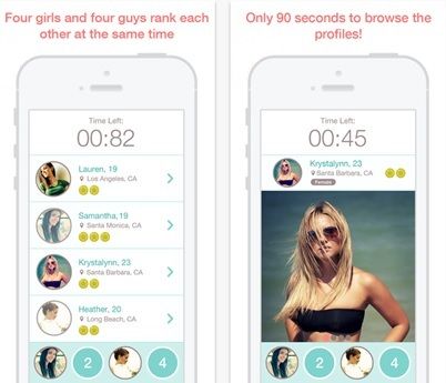
2Figure 1: Screen shot of the app during a game (from the perspective of a male user). Players indicate their rank-
ordered preference for the players from the opposite sex by dragging their profile pictures into the circles labeled one
through four at the bottom of the app. In this example, the focal player has picked his first and third choices, and is yet
to decide his second and fourth choices.
message from the matched partner after the game, (3) likelihood of receiving a reply to a message
sent after the game. The main challenge here is that users who received high preference-rankings
in the past (and hence have higher stars now) are also likely to receive higher preference-rankings
now – not necessarily because of their star-rating, but due to their inherent attractiveness, which
may be unobservable to the researcher (e.g., great bio descriptions, fun-loving pictures). This can
give rise to an upward bias in our estimates of the effect of star-ratings if we use naive estimation
strategies. To overcome this challenge, we leverage the fact that a user’s star-rating is not static;
rather it changes over the course of our observation period as a function of her/his rankings in the
previous games. Specifically, we model the first demand measure using a fixed-effects ordered logit
model, and the latter two using fixed-effects binary logit models. In all these models, we allow
user-specific unobservables (i.e., the fixed-effects) to be arbitrarily correlated with star-ratings.
We find that, everything else being constant, three-star users receive lower preference-rankings
compared to two-star users during the game, i.e., popularity has a negative effect on preference-
rankings. We also find that ignoring endogeneity problems would lead us to draw the exact opposite
conclusion. Interestingly, the effect of star-rating is different in after-game outcomes. In particular,
three-star users are more likely to receive both first messages and replies after the game. Thus, users
respond differently to popularity information at different stages of the matching process.
Next, we focus on our second research question, regarding the source of the popularity effect.
3Here, we leverage the differences in the risk of rejection across the observed demand measures
and show that the negative effect of star-ratings during the game can be attributed to strategic
shading. When a user is ranking a potential partner during the game, she has uncertainty on whether
that person is actually interested in a conversation/date. Indeed, even conditional on matching,
post-match rejection is very common (i.e., the matched partner does not initiate or respond to
messages).2 In contrast, in the reply message case, the user has already received a message from
her/his match and is considering whether to reply or not. Here, rejection is not a concern at all since
the other party has already expressed interest. Using the fact that the effect of star-rating in the reply
case is strictly positive, we show that the negative effect of star-rating during the game can stem
from strategic shading, which can be attributed to post-match rejection concerns. Further, we show
that the negative effect of star-ratings on preference-rankings is mainly driven by users who have
not had many successful conversations in the past. Since users with a history of being rejected are
more likely to have rejection concerns, this finding corroborates our strategic shading hypothesis.
In sum, our paper makes three contributions to the literature. First, we document negative
returns to popularity information in two-sided dating markets. Past empirical research has mainly
documented positive returns to the revelation of popularity information in e-commerce markets.
We show that those results do not always translate to two-sided matching markets where there are
rejection concerns (even when the matching is centralized). Second, we are the first to provide
empirical evidence for strategic shading in dating markets and directly link it to rejection concerns.
While strategic shading has been discussed in the literature, none of the earlier papers have been
able to causally identify it. Finally, centralized matching markets have long been proposed as a
panacea to the problems that plague decentralized markets. Our findings suggest that centralized
matching markets can still lead to strategic behavior if users have post-match rejection concerns.
Hence, markets where it is not feasible to enforce binding matches (e.g., dating markets, freelance
markets) may suffer from strategic behavior even with centralized matching.
2 Related Literature
First, our paper relates to a large stream of literature that has established that popularity information
has a positive effect on demand/sales of products and services in a variety of e-commerce settings,
such as the music industry (Salganik et al., 2006; Dewan et al., 2017), books (Sorensen, 2007),
restaurants (Cai et al., 2009), software downloads (Duan et al., 2009), kidney transplant market
(Zhang, 2010), movies (Moretti, 2011), digital cameras on Amazon (Chen et al., 2011), and the
2
Note that even though our setting constitutes a centralized market, there remain significant post-match rejection
concerns. In this aspect, our setting is unlike standard centralized matches where matches are binding, e.g., residents
and hospitals in NRMP program (Roth and Sotomayor, 1990).
4wedding services market (Tucker and Zhang, 2011).3 These studies have identified three mechanisms
for this positive effect: (1) observational learning or quality inference based on others’ actions (e.g.
purchase statistics), (2) salience effect or awareness of alternative choices, and (3) network effect or
increase in value of a product/service as its user base expands. In this paper, we provide the first
negative effect of popularity information on demand in an online marketplace, and in a previously
unstudied context – a two-sided dating market. We also present evidence for a new mechanism that
can moderate the effect of popularity information – strategic shading due to rejection concerns.
Second, our paper relates to the literature on the empirical measurement of mate preferences in
marriage and dating markets. Early work in this stream mostly used data on observed marriages to
estimate population-level mate preferences under the assumption of no search frictions (Wong, 2003;
Choo and Siow, 2006). More recently, researchers have been able to access data from speed-dating
and online dating platforms. In these settings, search frictions are minimal and researchers have
direct visibility into the search process employed by users and their preferences. This has led to a
stream of literature that attempts to directly estimate users’ preferences for mates along a variety of
dimensions, e.g., age, income, race, physical attractiveness (Kurzban and Weeden, 2005; Fisman
et al., 2006, 2008; Eastwick and Finkel, 2008; Hitsch et al., 2010a,b; Shaw Taylor et al., 2011;
Bapna et al., 2016; Lee, 2016a; Jung et al., 2019).
An important concern when measuring user preferences is the possibility of strategic behavior –
users may shade down their revealed preference for appealing users (physically attractive, popular,
etc.) to avoid the psychological cost of being rejected (Cameron et al., 2013). If users shade their
revealed preferences, and we do not explicitly account for this in the estimation, then our estimates
of user preferences will be biased. The effect of users’ perceived probability of being rejected on
their revealed preference has been examined by a few papers. In an early paper, Hitsch et al. (2010b)
employ empirical tests and show that strategic shading is not a concern in their setting. However,
their results may not hold if we have variables that directly affect the perceived risk of rejection (e.g.,
popularity information). We use the difference in the perceived risk of rejection across outcomes
(within-game ranking behavior and post-game reply behavior), and show that users strategically
shade their ranking for popular users because of rejection concerns. Fong (2020) shows that an
increase in market size increases selectivity while an increase in competition decreases selectivity.
However, this is conceptually different from the strategic shading that we document, where users
3
A related stream of work examines the effect of WOM or online reputation on demand outcomes (Chevalier and
Mayzlin, 2006; Sun, 2012; Yoganarasimhan, 2012, 2013). However, in these papers, ratings are given after the
interaction between the buyer and seller, and therefore help resolve asymmetric information on the quality of the
product/seller. In contrast, in our case ratings are purely measures of popularity and do not convey any information on
the unobserved quality of the user.
5strategically avoid popular and desirable mates because of rejection concerns, which in turn leads to
negative returns to popularity signals in dating markets.
Finally, our work relates to the literature on two-sided matching markets. There are two types of
two-sided matching markets: centralized and decentralized. In decentralized markets, there is no
central match-maker for the matching process. Instead, each agent engages in her/his own search
process, and makes/accepts offers over a period of time. It has been shown that these markets are
prone to market failures that can lead to inefficient matching because of search costs, unraveling,
and/or congestion (Roth, 2008; Niederle and Yariv, 2009). In particular, congestion can cause users
to strategically avoid making offers to their top preferences because of rejection concerns (Roth and
Xing, 1997; Che and Koh, 2016; Arnosti et al., 2019).
Centralized markets have long been proposed as the panacea to the problems plaguing decen-
tralized matching (Roth and Sotomayor, 1990). In their seminal work, Gale and Shapley (1962)
proposed an algorithm that requires users to submit rank-ordered lists of their preferences for the
opposite sex, and allocates stable matches for all users. Versions of this algorithm are used today
in centralized markets such as National Residency Matching Program (to match residents and
hospitals), and for matching students with public schools in New York City and Boston (Roth, 2008;
Abdulkadiroğlu and Sönmez, 2013). Our work contributes to the matching literature by showing
that centralized markets can still lead to preference-shading and strategic behavior if agents matches
are non-binding and there are non-negligible costs of being rejected.
3 Setting
3.1 Mobile Dating App
Our data come from a popular online dating iOS mobile application in the United States. The app
(or platform) is targeted at a younger demographic, and those using it are often looking for a fun
chat rather than long-term dating/marriage partners. To join and use the app, users need a Facebook
ID. When the user first logs in to the app (using his/her Facebook ID), the user’s name, gender, age,
education and employment information, and Facebook profile picture are automatically imported
from his/her Facebook account into the user’s dating profile in the app. Users cannot change this
information in their dating profile directly.4 However, they can upload up to five more pictures, and
add a short bio to their profile. Further, the app has access to a user’s real-time geographic location
(based on the GPS in the mobile device) when the user is actively using the app.
The app requires users to participate in a structured matching game, which is described in detail
below. Users cannot directly access or browse other users’ profiles through the app; the only way to
4
The app did not update this information (from Facebook) during our observation period.
6use the app is to play the ranking game described in §3.2.
3.2 Description of the Game
3.2.1 Game Assignment
Initiation and completion of a game requires the live participation of four men and four women.
When a user logs in to the app and decides to play a game, s/he is assigned to a game-room by
the platform. Among the available players, only two criteria are used by the platform to assign
players to games – proximity in geographic location and age. The exact algorithm is as follows: the
geographic location of the first player assigned to a game-room is set as the initial center point of
that game; the next player is then assigned to that game if he/she is within 500 miles of this center
point. The center point is then updated as the average location of the first two players. The third
player assigned to the game has to be within 500 miles of the new center point and after s/he is
assigned to the game, the geographic center is again updated. This continues until four men and four
women have been added to the game. Similarly, the platform ensures that the age gap between any
two members in a game is no more than six years (older or younger). In the data, we find that this
constraint is trivially satisfied because a vast majority of players belong to a small age bandwidth.
Therefore, conditional on geography and age, the assignment of users to games is random.
3.2.2 Game Activity
When a game starts, participants can see a list of four short profiles of the members of the opposite
sex. As shown in the left panel of Figure 1, these short profiles display a thumbnail version of users’
profile picture, name, age, location and their star-rating. Tapping on the thumbnail leads to the full
profile of the user (right panel of Figure 1), which contain a larger version of the profile picture (and
possibly additional photos) and other information, such as bio, education, and employment. Each
user then indicates his/her rank-ordered preference for the four members of the opposite sex. All
users have exactly 90 seconds from the start of the game to finalize their rank-orderings.5
Two points are worth noting. First, players do not know the identities and attributes of the other
members of their own sex in the game, i.e., men (women) do not know which other men (women)
are in the same game. Second, players’ actions are simultaneous and private, i.e., each user only has
visibility into his/her own actions and at no point is the rank-ordering of the other players revealed
to them (though they may be able to make some inferences after the game based on their match
assignments). Hence, while choosing their rank-orderings, they cannot use information on other
players’ preferences to make their own choices.
5
If one or more users leave the game or do not complete their rank-ordering, the game is deemed incomplete and no
matches are assigned. In our data, we see a very high rate (over 97%) of game completions.
7Figure 2: Screen shots of the application before and after a game.
3.2.3 Match Allocation
The platform uses the rank-ordered preferences of all players in a game to derive a set of “stable
matches”, where the concept of stability is based on the canonical Stable Marriage Problem (SMP):
“Given n men and n women, where each person has ranked all members of the opposite sex in order
of preference, match the men and women such that there are no two people of opposite sex who
would both prefer each other over their current partners,” (Gale and Shapley, 1962).
There are a few noteworthy points about the SMP. First, for any combination of preferences,
there always exists at least one solution/stable match to a SMP. Second, the SMP can have more than
one solution even for a relatively small number of players and the optimality of these solutions can
depend on the algorithm used. For instance, Gale and Shapley (1962) show that a “Men-proposing
Gale-Shapley Deferred Acceptance algorithm” is men-optimal, i.e., none of the men can do better
under a different algorithm.6 In our case, the platform first calculates all possible solutions for
a game by considering all combinations of matches and checking for stability. If a game has a
unique solution, then the platform allocates matches based on this solution. If there are two or more
solutions, the solution that offers the highest average match is chosen. Thus, the platform does not
optimize for either men or women, but instead tries to pick the best globally optimal solution.7
6
Similarly, a women-proposing Gale-Shapley Deferred Acceptance algorithm is women-optimal, i.e., none of the
women can do better using a different algorithm.
7
The average match of a solution is calculated as follows: take the ranking that each player gave the person s/he is
paired with in a stable match and sum this number over all players. In case there are multiple solutions with the same
average match, ties are broken randomly.
8The entire matching process takes less than a second and users can see the match assigned to
them as well as all the other matches allocated in the room (see the right panel of Figure 2).
3.2.4 Post-Game Actions
After they have been assigned a match, users have the option to send a message to their match;
see Figure 2 on the right panel. Users can also play another game, go to the home page or close
the app. However, if they choose any of the latter actions without first sending a message to their
matched partner, they lose the option to communicate with them in the future (unless the matched
person sends them a message, in which case they can respond to it and continue the conversation).
Once users initiate or receive a message, the message stays in their Inbox, and they can continue to
communicate with that person in the future, if they choose to. Finally, note that users cannot start or
receive any communication from other players in the game with whom they have not been matched.
4 Data
Our data comprises of 94,386 games played by 24,653 unique users during the ten month period
from September 15th 2014 to July 15th 2015. The data can be categorized into three groups: (1)
User-level data, (2) User-User level data, and (3) User-Game level data. We now describe the
variables in each of these categories and present some summary statistics on them.
4.1 User-level Data
We first describe the time-invariant attributes associated with each user i.
• genderi : A dummy variable indicating user i’s gender; is 1 for men and 0 for women.
• agei : User i’s age.8
• bioi : The length of user i’s bio in his/her profile (i.e., number of words).
• educationi : Categorical variable that denotes the user i’s highest education level (either earned
or working towards), where 1 = High-school, 2 = College, and 3 = Graduate school.
• employmenti : Number of positions/companies mentioned in user i’s profile.
• initial gamei : Total number of games played by user i before the data collection period.
• total gamei : Total number of games played by user i during the data collection period.
• num pici : Number of uploaded pictures in the dating profile.
In addition, we also have access to the profile picture of user i. To obtain a measure of the physical
attractiveness of a user’s profile picture, we conducted a survey. We asked 384 heterosexual subjects
in a research lab to rate the profile pictures of the opposite sex (men rated women and vice-versa),
8
Age (calculated based on the user’s Facebook birthday) changes for 26.87% users (6,378 users) during our sample
period. However, this is a deterministic change i.e., age can increase only by one in the 10-month window.
9Variables Mean Std. Dev 25th 50th 75th (Min, Max) Size
agei 21.53 5.41 19 21 22 (13, 109) 22024
bioi 67.04 275.58 0 0 63 (0, 29519) 22948
employmenti 1.29 1.60 0 1 2 (0, 68) 24653
initial gamei 59.50 64.32 0 48 90 (0, 2146) 24653
total gamei 31.27 37.90 6 18 45 (1,1069) 24653
num pici 4.26 1.01 4 4 4 (0, 6) 22669
pic scorei 0.00 0.68 -0.52 -0.09 0.43 (-2.88, 3.29) 17739
genderi (0) female: 42.45% (1) male: 57.55% 24653
educationi (1) high-school: 19.24% (2) college: 78.12% (3) graduate: 2.64% 21604
Table 1: Summary statistics of user-level data.
on a scale of 1 to 7, with 1 being “not at all attractive” and 7 being “very attractive”. The subjects
were undergraduate students at a large state university in the west coast, with an equal fraction of
male and female, and their ages ranged between 18-25 (with a median age of 21). This demographic
distribution closely mimics the age and gender distribution of the app users.
During the lab study, each subject rated 100 randomly pictures in approximately 20 minutes. On
average, each profile picture was rated by five subjects to ensure that the ratings captured average
appeal rather than idiosyncratic preferences of a specific subject. It is possible that some subjects
give consistently higher or lower ratings than other subjects. We therefore standardized each rating
by subtracting the mean rating given by the subject and dividing by the standard deviation of the
subject’s ratings, as advocated by Biddle and Hamermesh (1998). We then take the average of all
the standardized ratings that user i’s picture received in our study and denote it as:
• pic scorei : The average physical attractiveness score of user i’s profile picture.
Finally, because of constraints in subject-pool time, we could only obtain the picture-scores for a
random sub-sample of users instead of the full pool of users; thus we have picture-score information
for 17,753 of the 24,653 unique users.
The summary statistics of all the user-level variables are shown in Table 1. Of the 24,653 users,
14,189 (57.55%) are male and 10,464 (42.45%) are female. The median user is 21 years old, has no
bio written on her/his profile, has/is working towards a college degree, and one employment-related
information is listed on her/his profile. S/he has played 48 games before the data collection period
and plays 18 games during it. However, there is quite a bit of variation across users in the extent of
activity, with some users playing over 1000 games during our observation period.
Finally, note that the above user-specific variables are treated as time invariant because users lack
the ability to change most of their profile information after it is first imported from their Facebook
profile (name, gender, age, education and employment information, and profile picture). The two
pieces of information that users can change in the app are – (1) the five extra pictures that they are
10allowed to upload (in addition to the profile picture), and (2) their short bio. However, we do not
believe that this was a frequent occurrence for the reasons discussed in §6.3.2.
4.2 User-User level data
Each game consists of eight unique users – four men and four women. For each man-woman pair in
a game, we have data on the preference-ranking that they gave each other, their match outcome, and
their post-match interactions. We describe these variables in detail below.
• prefijt : The preference-ranking that user i receives from user j in game t; it can take values
from one to four, with four indicating the highest preference and one the lowest.
Users rank members of the opposite sex from one through four (as shown in Figure 1), with a
rank of one indicating their highest preference and four indicating the lowest. We convert these
rank orderings to preference-rankings, such that rank of one denotes a preference-ranking of
four, rank of two indicates a preference-ranking of three, and so on. The transformed variable
pref is easier to interpret because higher values of this variable correspond to more preference.
• matchijt : A dummy variable indicating whether user i is matched with player j in game t. In
each game, all players are uniquely matched with one other player from the opposite sex. So for
woman (man) i in a game, this variable is equal to one for only one man (woman).
• firstijt : A dummy variable indicating whether user i receives the first message from the matched
partner (denoted by j) after game t. Since users cannot communicate with players that they
have not been matched with, by default, this variable is zero if matchijt = 0.
• replyijt : A dummy variable indicating whether user i receives a reply message from the matched
partner j after game t, conditional on user i initiating the first message. By default, this variable
is zero if firstjit = 0.
The summary statistics of these variables are shown in Table 2. The sample sizes of pref and
match reflects the fact that there are 32 observations per game.9 The distributions of pref and
match are determined by the game structure, and their summary statistics are as expected. The
sample size of firstijt reflects the fact that there are eight users matched with each other, and each
of them can potentially initiate the first message. It is worth noting that the mean of firstijt is
around 0.05 (of the 713,014 matches, only 39,377 messages were initiated). The observed number
of first messages (39,377) defines the sample size of replyijt . The mean of replyijt is around 0.08
(among 39,377 first messages only 3380 receive a reply). Interestingly, 76% of the conversations are
9
Eight users participate in each game and each user receives four preference-rankings from players of the opposite sex.
So we have a total of 8 × 4 = 32 preference-rankings per game. Also, since each user can be matched with only one of
the four potential mates, matchijt becomes one once and zero thrice. Thus, for each game we have 8 × 1 + 8 × 3 = 32
data points for matchijt . Therefore, the size of prefijt and matchijt should be the number of games (94,386) × 32 =
3,020,652. However, there were some discrepancies in the data for 42 users, so we exclude them from our analysis.
11Variables Mean Std. Dev 25th 50th 75th (Min, Max) Size
prefijt 2.5 1.12 2 3 4 (1, 4) 3008560
matchijt 0.25 0.43 0 0 0.5 (0, 1) 3008560
firstijt 0.05 0.23 0 0 0 (0, 1) 713014
replyijt 0.08 0.28 0 0 0 (0, 1) 39377
Table 2: Summary statistics of user-user level data.
initiated by men, which indicates that women are less likely to approach men after being matched.
Further, men receive a reply to their messages 5% of the times, and women receive a reply 20%
of the times. These statistics are consistent with previous research on online dating, which find
that men are more likely to initiate contact and respond to emails/messages, compared to women
(Kurzban and Weeden, 2005; Fisman et al., 2006; Hitsch et al., 2010b).
4.3 User-Game level data
We now describe user-game level variables, i.e., user-specific data that varies with each game.
• match levelit : An integer variable that denotes how much user i prefers his match in game t.
match levelit = prefjit where matchijt = 1 (1)
• total gameit : Total number of games that user i has played before game t. This is updated by
one after each game played by user i.
• starit : Indicates the user’s star-rating in game t; see Figure 1 for an example. User’s star-rating
is updated in real time after each game and is calculated as follows:
1, if 1 ≤ popularityit < 2
starit = 2, if 2 ≤ popularityit < 3 (2)
if 3 ≤ popularityit ≤ 4,
3,
where popularity is defined as the average of the preference-rankings that user i has received
Ptotal gameit P4
prefijq
before the tth game, such that popularityit = q=14×total game j=1
it
. While users know their
own star-rating before each game, and members of the opposite sex in the game room can
observe a user’s star-rating, the platform does not reveal a user’s popularity scores to her/him or
to anyone else in the platform.
Figure 3 illustrates the relationship defined in Equation (2). Intuitively, an individual’s star-
rating captures how popular or sought after s/he was in her/his past games. Three-star users, on
average, are those who were among the top two choices of other players. Two-star players are
those who, on average, were the second or third choice of players in the past . Finally, one-star
121 2 3 4
popularityit
Figure 3: Pictorial representation of the star-rating rule.
Variables Mean Std. Dev 25th 50th 75th (Min, Max) Size
match levelit 3.19 0.95 3 3 4 (1, 4) 752140
total gameit 74.75 74.25 29 59 97 (0, 2194) 752140
starit 2.00 0.10 2 2 2 (1,3) 745037
Table 3: Summary statistics of user-game level variables.
players, on average, are those who were the third or fourth choice of others in the past. Thus,
there is a clear monotonic relationship between past popularity and current star-rating.
The summary statistics of all the user-game level variables are shown in Table 3. There are a
few interesting points of note. First, the average match level is 3.19, which implies most users
get matched with their first or second top choices, on average.10 We also find that the median of
total gameit is 59, i.e., most users have played a good number of games before a median game in
the observation period. Moreover, we see that users are shown with a two-star rating on average.
Finally, we examine the within-user variation in star-ratings. Of the 24,653 users in our data,
85.83% (21,159 users) are shown with two stars in all their games, i.e., they never experience a star
change. However, 3,494 users experience a star change. Of these, 36.83% (1,287 users) were shown
with a minimum of one star and a maximum of two stars, and 62.54% (2,185 users) were shown
with a minimum of two and maximum of three stars. Very few users (22) experienced a minimum
of one star and a maximum of three stars. In sum, while a majority of users never experience a star
change, there is a sufficiently large portion that goes through at least one star change.
10
If user i is matched with her most preferred player in game t, then in that game, match levelit = 4, and if she is
matched with her least preferred player, match levelit = 1. If preferences were purely vertical, i.e., if all the men in
a game had the same rank-ordering for women (and vice-versa), and users report their preferences without strategic
shading, then the mean match level would be 2.5. Instead, if preferences were purely horizontal, then the mean
match level would be 4. The fact that the average of match level is 3.19, suggests that users’ preference-rankings
are a combination of vertical attribute, horizontal attributes, and other factors such as strategic shading.
135 Descriptive Analysis
We now examine the relationship between a user’s star-rating and three measures of her/his demand
– preference-rankings received during the game, and whether s/he receives a first message, or reply
message after the game – using simple model-free analyses. In this section, we focus on users who
experienced at least one change in their star-rating during our observation period.
The relationship between a user’s star-rating in a given game and the average preference-
ranking that s/he receives in that game is illustrated in Figure 4. The solid increasing line shows
the relationship between the average preference-rankings received for all user-game observations
calculated for each star-rating.11 We see that in observations where users have higher star-ratings,
they also receive higher preference-rankings. However, there is an obvious issue of correlated
unobservables here, i.e., users with higher star-ratings are likely to be more attractive on other
unobserved dimensions (e.g., physical attractiveness) as well. To examine if this conjecture is true,
we plot the average of users’ pic score for each star-rating. As shown in Figure 5, users with higher
star-ratings also have higher physical attractiveness score, on average. Thus, the effects shown by
the solid line in Figure 4 cannot be interpreted as causal.
3 0.2
0.1
pic_score
2 0
pref
-0.1
1 -0.2
star1 star2 star3 star1 star2 star3
Figure 4: Relationship between star-ratings and Figure 5: Relationship between star-ratings and
average preference-rankings received. average physical attractiveness score.
One way to cleanly capture the effect of star-ratings is to look at the effect of star-ratings within
an individual, i.e., if we compare preference-rankings received by the same individual when s/he is
shown with different star-ratings, then our comparisons are less likely to be subject to endogeneity
concerns. Consider an individual who was shown with a minimum of one star and a maximum
of two stars and calculate two averages: (1) the average of preference-rankings received in games
where s/he is shown with one star, and (2) the average of preference-rankings received in games
P P P
11 i (prefijt | starit =1)
tP jP
For example, the average preference-ranking for the data point at star1 on the solid line is 4× i t I(starit =1) .
14where s/he is shown with two stars. We then perform an analogous exercise for users who were
shown with a minimum of two stars and a maximum of three stars. These two comparisons are
shown using dashed lines in Figure 4. As we can see, on average, the same set of users receive
higher preference-rankings when they are shown with one star compared to two stars. Moreover, on
average, the same set of users receive higher preference-rankings when they are shown with two stars
compared to three stars. This implies that higher star-ratings leads to lower preference-rankings,
i.e., users avoid those with higher stars! Note that the direction of the effect of star-rating on
preference-rankings in solid line and dashed lines in Figure 4 are exactly opposite. This discrepancy
implies that controlling for the endogeneity between star-ratings and unobserved factors that affect
user attractiveness is essential to deriving the causal impact of star-ratings in our setting.
Next, we conduct an analogous analysis on the relationship between a user’s star-rating and the
likelihood of receiving the first message and receiving a reply if s/he initiates a message, and present
the results in Figures 6 and 7. First, we see that observations where users have higher star-ratings
are more likely to receive both first messages and replies (solid lines in the figures). Second, for
the within-user analysis, we see that, on average, the same set of users are more likely to receive
first messages when they are shown with one star compared to two stars (though this is not the case
when we compare two and three stars). In the case of reply, the same set of users are more likely to
get a reply when shown with higher star-ratings.
Figure 6: Relationship between star-ratings and the Figure 7: Relationship between star-ratings and the
average likelihood of receiving the first message. average likelihood of receiving a reply message.
In sum, when we look at the simple correlation between star-ratings and revealed preferences,
we always see a positive effect. However, when we look at within-individual comparisons, the
findings are quite different. Interestingly, the effect of higher star-ratings seems to be negative for
preference-rankings during the game, partially-negative for initiating communication after the game
(first message), and positive when it comes to replying to messages after the game. In the rest of
15the paper, we focus on deriving the unbiased causal effect of star-ratings on these three revealed
preference measures, and exploring the mechanisms driving these effects.
6 Effect of Star-ratings on Preference-Rankings
In this section, we formalize the causal impact of a user’s star-rating on the preference-rankings that
s/he receives during the game. In §6.1 and §6.2, we present the model specification and estimation.
In §6.3, we discuss the identification and we discuss our findings in §6.4.
6.1 Model Specification
The outcome variable of interest here is prefijt , which denotes the preference-ranking that user i
receives from j during game t. Note that pref is an ordinal integer value going from 1 to 4, with
one representing the lowest preference-ranking and four indicating the highest preference-ranking.
Therefore, we use an ordered logit model12 that relates the observed outcome variable prefijt to a
latent variable prefijt∗ where:
prefijt∗ = β1 star1it + β2 star3it + γzi + ηi + ijt , (3)
The latent variable prefijt∗ is modeled as a linear function of:
• star1it , star3it – indicator variables for the star-rating of user i in game t, where star2it is
considered as the base.
• zi – set of user-specific observables that can affect j’s ranking of i, e.g., gender of i.
• ηi – set of unobservable (to the researcher) characteristics of user i that is visible to j and affects
j’s ranking of i. These could include the aspects of user i’s physical attractiveness not captured
in our lab study (e.g., other photos of the user), details in her/his bio description, employment
details, her geographic location, etc.
• ijt – factors uncorrelated to the star-rating of user i that can affect the preference-ranking s/he
receives from j in game t. We assume that ijt s have a logistic cumulative distribution. Three
key sets of variables are subsumed in ijt . First, it includes j’s attributes (both observable zj and
unobservable ηj ) since there is no correlation between j and i’s attributes. Second, it includes
all the attributes of the other three players of i’s gender who i is being compared with, in game
t.13 The reason neither of the above two sets of variables affect our inference on star-ratings
is because the app adds users into a game randomly. Thus, there is no correlation between the
12
We discuss other modeling frameworks such as rank-ordered logit or Regression Discontinuity Design (RDD) in
Appendix §A and explain why they are not appropriate for our setting.
13
Including the observations of all the competitors in a game can create within-game correlation in our analysis. We
address this issue in §8.3.
16attributes of users within a game.14 Third, it can capture idiosyncratic factors that affect j’s
ranking of i within the game, e.g., j’s mood for going on a date with someone of i’s type etc.
We then model the relationship between prefijt and prefijt∗ as follows:
prefijt = k if µk < prefijt∗ 6 µk+1 ∀ k = 1, 2, 3, 4, (4)
where the thresholds µk are strictly increasing. Further, we assume that µ1 = −∞ and µ5 = ∞.
This specification is the ordinal choice analog of a binary logit model. Thus, prefijt can take four
possible values, denoted by k. Because the error terms are drawn from a logistic distribution, we
can write the cumulative probability function of ijt as
1
F (ijt | Xit , β1 , β2 , γ, ηi , µk , µk+1 ) = ≡ Λ(ijt ), (5)
1 + exp(−ijt )
where Xit = {star1it , star3it , zi }. Therefore, the probability of observing outcome k in game t for
a pair of users (where user i receives a rank k from user j) can be written as:
P r pref ijt = k | Xit , β1 , β2 , γ, ηi , µk , µk+1 = Λ (µk+1 − β1 star1it − β2 star3it − γzi − ηi )
− Λ (µk − β1 star1it − β2 star3it − γzi − ηi ) (6)
Using this model formulation, we can then write the log-likelihood of the preference-rankings
observed in the data as:
X Ti X
N X 4 X
4 h i
I(prefijt =k)
LL(β1 , β2 , γ, ηi , µk , µk+1 ) = ln P r (prefijt = k | Xit , β1 , β2 , γ, ηi , µk , µk+1 ) ,
i=1 t=1 j=1 k=1
where N is the total number of users observed and Ti is the total number of games played by user i.
The unknown parameters in Equation (7) are β1 , β2 , γ, ηi s, µ2 , µ3 , µ4 .
6.2 Estimation
We are mainly interested in estimating the effect of star-ratings (β1 and β2 ). The challenge comes
from the potential correlation between ηi and starit , i.e., we expect that E[starit · ηi ] 6= 0. We now
discuss three estimation strategies that address this problem in varying degrees.
14
In principle, because the app only adds new users within a 500 mile radius of users already in the game, the geographic
locations of users in a game are correlated. However, conditional on being in the same room, there is no correlation
between the location of two users, and the distance between the users is random. In other words, if we denote the
geographic location of users by g, then we can write the location of j as: gj , where gj = gi + δ, where gi , gj , δ are
two dimensional vectors (latitude, longitude) such that ||gj − gi ||≤ 500. Since we already control for user i’s location
(gi ) through ηi , the remaining δ is random noise.
17First, a pooled ordered logit model, which ignores the user-specific unobservables ηi . It simply
involves pooling all the user-game data, ignoring the user-specific variables (zi , ηi ), and then
maximizing the log-likelihood in Equation (7). However, it is important to recognize that the
estimates from this approach will be biased in the presence of correlated unobservables.
Second, a pooled ordered logit model with control variables, that includes user-specific variables
(zi ) to control for the correlation between starit s and ηi . For example, controlling for users’ physical
attractiveness (pic scorei ) may reduce the bias in estimates of β1 and β2 . However, this method is
unable to control for the correlation between starit s and ηi .
Third, a fixed-effects ordered logit model, where we allow the user-specific unobservables ηi to
be arbitrarily correlated with the star-ratings. A naive approach to estimation with fixed-effects is
to treat the ηi ’s as parameters and maximize the log-likelihood in Equation (7) directly. However,
such a Maximum Likelihood Estimator (MLE) is inconsistent with large N and finite T due to the
well-known incidental parameters problem (Neyman and Scott, 1948). As a result, the estimates
of β1 and β2 from this approach will be inconsistent too. Chamberlain (1980) provides an elegant
solution to the incidental parameters problem by dichotomizing the ordered outcome variable. In
§6.2.1, we describe how to apply the Chamberlain estimator to our setting, in §6.2.2 we describe
how the Chamberlain estimators can be combined to form an efficient Minimum Distance estimator.
6.2.1 Chamberlain’s Conditional Maximum Likelihood Estimator
The ordered outcome variable prefijt can take K = 4 possible integer values, {1,2,3,4}. Therefore,
we can transform the random variable prefijt into K − 1 = 3 possible binary variables prefijtk where:
prefijtk = I(prefijt ≥ k), where k = 2, 3, 4. (7)
For example, the binary variable prefijt4 indicates whether user i received a preference-ranking of 4
from user j in game t, or not. Similarly, the binary variable prefijt3 indicates whether user i receives
a preference-ranking of 3 or higher (i.e., 3 or 4) from user j in game t, or not. We can specify
Chamberlain’s Conditional Maximum Likelihood (CML) estimator on each of these transformed
binary variables. For each k, prefijtk is a binary logit variable such that:
P r(prefijtk = 1 | Xit , β1 , β2 , γ, ηi , µk ) = 1 − Λ(µk − β1 star1it − β2 star3it − γzi − ηi ) (8)
We denote prefik as the entire history of preference-rankings at level k received by user i over time,
i.e. prefik = {prefi11
k k
, prefi21 k
, prefi31 k
, prefi41 k
, ..., prefi1T i
k
, prefi2Ti
k
, prefi3T i
k
, prefi4Ti
}. Further, let
k
si be the sum of all the binary transformed preference-rankings at level k received by user i such
that ski = Tt=1
P i P4 k k k
j=1 prefijt . In other words, si shows the count of ones in the set of prefi . Let
18Bik be the set of all possible vectors of length 4 × Ti with ski elements equal to 1, and 4 × Ti − ski
elements equal to 0.15 That is:
Ti X
X 4
Bik = {d ∈ {0, 1} 4×Ti
| djt = ski } (9)
t=1 j=1
Now, we can write the conditional probability of prefik given ski as:
exp prefik · (β1 star1it + β2 star3it )
P r prefik | star1it , star3it , ski , β1 , β2
=P (10)
d∈B k exp (d · (β1 star1it + β2 star3it ))
i
A key observation is that this conditional probability does not depend on ηi ’s (or the thresholds µk ’s
or zi ’s), i.e., ski is a sufficient statistic for ηi . Thus, we can now specify a Conditional Log-Likelihood
that is independent of ηi s and µk s as shown below:
Ti
N X
X
CLL(β1k , β2k ) ln P r(prefik | star1it , star3it , ski , β1k , β2k )
= (11)
i=1 t=1
Since we can dichotomize prefijt into three binary variables at each of the three cutoffs (pref 4ijt ,
pref 3ijt , and pref 2ijt ), the above CLL can be specified for each pref kijt , where k ∈ {2, 3, 4}. Max-
imizing each of these CLLs gives us three separate but consistent estimates of β1 , β2 , which we
denote as {β1k , β2k }, where k ∈ {2, 3, 4}. These are referred to as Chamberlain CML estimators.
However, these three estimates are inefficient because each of them only uses part of the variation
in the data for identification. Intuitively, at any cut-off k, only the variation around k is used for
identification because of dichotomization; for example, the CLL for k = 4 only considers whether
prefijt is greater than or equal to 4 and ignores the variation in prefijt when it is less than 4. Thus,
while Chamberlain’s CML estimator at each k is consistent, it is not efficient because it does not
exploit all the variation in data.16
4×Ti
15
Note that the size of Bik = sk
. Consider user i who plays two games (Ti = 2). For k = 4,
i
4
we have pref ijt ∈ {0, 1} that denotes whether user i has received a preference-ranking of 4 from user j
or not. Now, let’s consider a scenario where user i receives a preference-ranking of four only in her first
game and from j1 , i.e. , prefi4 = {1, 0, 0, 0, 0, 0, 0, 0}. Thus, s4i = 1. Next, we can write Bi4 or
the set of all possible ways that user i can get only one preference-ranking of 4 in her games by Bi4 =
{(1, 0, 0, 0, 0, 0, 0, 0), (0, 1, 0, 0, 0, 0, 0, 0), ..., (0, 0, 0, 0, 0, 0, 1, 0), (0, 0, 0, 0, 0, 0, 0, 1)}. Note that each element of
Bi4 is itself a vector with eight elements, because user i has played two games and in each game s/he receives four
preference-rankings(4 × 2 = 8). We denote each element of set Bi4 with vector d. Also, notice that the size of Bi4 is
eight, because 4×2 1 = 8.
16
For individuals who have played a large number of games (large Ti ) and have a large number of positive values of
pref kijt (large ski ), calculating all combinations of outcomes can lead to numerical overflow and computational issues.
196.2.2 Minimum Distance Estimator
To address the efficiency issue in Chamberlain’s CML, Das and Van Soest (1999) proposed a
Minimum Distance (MD) estimator that combines all the Chamberlain estimates. We now describe
the application of their method to our context. Recall that we have K − 1 = 3 estimates for each
of {β1 , β2 }: {β11 , β21 }, {β12 , β22 }, {β13 , β23 }. Since each of these three estimates are consistent, any
weighted average of these estimates will be consistent too. The main idea in Das and Van Soest
(1999) is to use the variance and co-variances of K − 1 estimators as weights and generate one
efficient estimate. It thus involves solving the minimization problem:
β̂ M D = argmin(β̃ − M b)0 var(β̃)−1 (β̃ − M b), (12)
b
where β̃ is the 6 × 1 matrix of Chamberlain estimators, M is the matrix of 3 stacked 2-dimensional
identity matrices, and var(β̃) is the variance-covariance matrix of the stacked Chamberlain estimates.
In other words, we need to find b1 and b2 such that:
0 −1
β˜12 − b1 var(β˜12 ) β˜12 − b1
˜2
β2 − b2 cov(β˜22 , β˜12 ) var(β˜22 )
˜2
β2 − b2
β˜3 − b . . var( ˜3 )
β β˜3 − b
1 1
argmin ˜13 1
1
b1 ,b2 β − b
. . . var( ˜
β 3
)
˜3
β − b
2 2
2
2 2
β˜4 − b . . . . var( ˜4 )
β β˜4 − b
1 1 1 1 1
˜ 4
β2 − b2 ˜4 ˜2
cov(β2 , β1 ) . . . ˜4 ˜4 ˜4
cov(β2 , β1 ) var(β2 ) ˜ 4
β2 − b2
The solution to the above minimization problem (b1 and b2 ) is a weighted average of the Chamberlain
estimators and is equal to:
β̂ M D = {M 0 var(β̃)−1 M }−1 M 0 var(β̃)−1 β̃ (13)
and its variance is given by var(β̂ M D ) = {M 0 var(β̃)−1 M }−1 . We implement this MD estimator
using the Stata code developed by Hole et al. (2011). For more details about this method and a
comparison with other methods, see Baetschmann et al. (2015).
For example, if user iplays 100 games (Ti = 100) and receives one preference-ranking of four in each game, then
s4i = 100 and 4×100
100 = 2.24e + 96. Therefore, we limit our empirical analysis to users’ first 100 games. Of the
3,494 users who experience a star change, only 352 (10%) users play more than 100 games. The consistency of the
estimates is not affected if we choose a subset of games for players who have played a large number of games.
20You can also read