Modeling the marine chromium cycle: new constraints on global-scale processes - Climate and ...
←
→
Page content transcription
If your browser does not render page correctly, please read the page content below
Biogeosciences, 18, 5447–5463, 2021
https://doi.org/10.5194/bg-18-5447-2021
© Author(s) 2021. This work is distributed under
the Creative Commons Attribution 4.0 License.

Modeling the marine chromium cycle: new constraints on
global-scale processes
Frerk Pöppelmeier1,2 , David J. Janssen2,3 , Samuel L. Jaccard2,3,4 , and Thomas F. Stocker1,2
1 Climate   and Environmental Physics, Physics Institute, University of Bern, 3012 Bern, Switzerland
2 Oeschger   Center for Climate Change Research, University of Bern, 3012 Bern, Switzerland
3 Institute of Geological Sciences, University of Bern, 3012 Bern, Switzerland
4 Institute of Earth Sciences, University of Lausanne, 1015 Lausanne, Switzerland

Correspondence: Frerk Pöppelmeier (frerk.poeppelmeier@climate.unibe.ch)

Received: 21 April 2021 – Discussion started: 18 May 2021
Revised: 3 August 2021 – Accepted: 31 August 2021 – Published: 7 October 2021

Abstract. Chromium (Cr) and its isotopes hold great promise       1   Introduction
as a tracer of past oxygenation and marine biological activity
due to the contrasted chemical properties of its two main ox-
idation states, Cr(III) and Cr(VI), and the associated isotope    The chromium (Cr) cycle at the Earth’s surface has received
fractionation during redox transformations. However, to date      continuous attention throughout the past decades to gain bet-
the marine Cr cycle remains poorly constrained due to insuf-      ter understanding on the mobility of hexavalent Cr (Cr(VI)),
ficient knowledge about sources and sinks and the influence       a carcinogenic pollutant in the environment (e.g., Wang et
of biological activity on redox reactions. We therefore imple-    al., 1997). More recently, research was further motivated by
mented the two oxidation states of Cr in the Bern3D Earth         technical advances in mass spectrometry that allow for ro-
system model of intermediate complexity in order to gain          bustly measuring the stable isotopic composition of Cr (e.g.,
an improved understanding on the mechanisms that modu-            Bonnand et al., 2013; Moss and Boyle, 2019; Wei et al.,
late the spatial distribution of Cr in the ocean. Due to the      2020), the fractionation of which is linked to redox trans-
computational efficiency of the Bern3D model we are able to       formations between its two main oxidation states Cr(III) and
explore and constrain the range of a wide array of param-         Cr(VI) (Ellis et al., 2002; Joe-Wong et al., 2019; Wanner and
eters. Our model simulates vertical, meridional, and inter-       Sonnenthal, 2013; Zink et al., 2010). This permitted the ap-
basin Cr concentration gradients in good agreement with ob-       plication of stable Cr isotopes as a proxy for past changes in
servations. We find a mean ocean residence time of Cr be-         oceanic and atmospheric oxygenation (e.g., Frei et al., 2009;
tween 5 and 8 kyr and a benthic flux, emanating from sedi-        Planavsky et al., 2014). Recent investigations revealed that
ment surfaces, of 0.1–0.2 nmol cm−2 yr−1 , both in the range      biologically mediated redox reactions may play an important
of previous estimates. We further explore the origin of re-       role in the marine Cr cycle (Huang et al., 2021; Janssen et
gional model–data mismatches through a number of sensitiv-        al., 2020; Semeniuk et al., 2016), and the isotopic ratios mea-
ity experiments. These indicate that the benthic Cr flux may      sured in marine sediments may hence be potentially used for
be substantially lower in the Arctic than elsewhere. In ad-       the reconstruction of past changes in biological productivity.
dition, we find that a refined representation of oxygen mini-        Yet, despite growing interest, the marine Cr cycle remains
mum zones and their potential to reduce Cr yield Cr(III) con-     poorly constrained (Wei et al., 2020). In particular, anthro-
centrations and Cr removal rates in these regions in much         pogenic Cr contaminations of rivers and coastal environ-
improved agreement with observational data. Yet, further re-      ments, insufficient knowledge about the redox behavior of
search is required to better understand the processes that gov-   Cr in the open ocean, as well as in oxygen minimum zones
ern these critical regions for Cr cycling.                        (OMZs) (Moos et al., 2020; Nasemann et al., 2020), and the
                                                                  possibility of yet unrecognized Cr sources from sediments
                                                                  (Janssen et al., 2021) complicate the understanding of the

Published by Copernicus Publications on behalf of the European Geosciences Union.
5448                                                                F. Pöppelmeier et al.: Modeling the marine chromium cycle

marine Cr cycle. This is also reflected in divergent estimates        investigate the impact of different parametrizations on OMZ
of the mean residence time of Cr in the ocean, which range            Cr reduction and removal pathways. The tightly constrained
from 2 to 40 kyr (McClain and Maher, 2016; Sirinawin et al.,          relationship between the dissolved Cr concentration and the
2000; Wei et al., 2018), further highlighting the lack of con-        stable isotopic ratio could ultimately allow for future model–
straints on source and sink apportionment.                            data intercomparisons using marine sedimentary isotope data
   In the modern ocean, total dissolved Cr concentrations of          to reflect past changes in the marine Cr cycle.
unpolluted waters typically range between 1 and 6 nmol kg−1
(e.g., Jeandel and Minster, 1987; Nasemann et al., 2020) of
which a majority (> 70 %) is generally found in the solu-             2     Model description and experiments
ble Cr(VI) redox state. Reduction of Cr(VI) is either induced
                                                                      2.1    Bern3D model
in poorly oxygenated waters or catalyzed by Fe(II) and or-
ganic matter in oxic waters (Janssen et al., 2020; Kieber             The Bern3D v2.0 EMIC (Roth et al., 2014) consists of a
and Helz, 1992). As such, Cr(III) concentrations can account          dynamic geostrophic-frictional balance model (Edwards et
for the majority of total dissolved Cr in OMZs (Huang et              al., 1998; Müller et al., 2006) featuring an isopycnal dif-
al., 2021; Rue et al., 1997) and may also be elevated in              fusion scheme and Gent–McWilliams parametrization for
high-productivity surface waters (e.g., Janssen et al., 2020).        eddy-induced transport (Griffies, 1998). The horizontal res-
Complexation with organic ligands may further increase its            olution comprises 40 × 41 grid cells with 32 logarithmically
solubility (e.g., Yamazaki et al., 1980). Trivalent chromium          scaled depth layers. The ocean model is coupled to a single-
is fairly particle reactive and is thus rapidly removed from          layer energy–moisture balance model on the same horizon-
the dissolved phase via adsorption on sinking particles with          tal grid (Ritz et al., 2011). Cloud cover and wind stress are
strong affinities for biological particles (Janssen et al., 2020;     prescribed from satellite re-analysis data of monthly clima-
Semeniuk et al., 2016; Wang et al., 1997). Hence, subsurface          tologies (ERA40; Kalnay et al., 1996). Biogeochemical cy-
pelagic Cr(III) concentrations away from OMZs are substan-            cling is implemented as described by Parekh et al. (2008) and
tially lower than Cr(VI) concentrations typically ranging be-         Tschumi et al. (2011). In brief, export production of particu-
tween 0.0 and 0.3 nmol kg−1 (Janssen et al., 2020). The re-           late organic matter (POM), calcium carbonate (CaCO3 ), and
dox behavior and the different particle affinities of the two         biogenic opal is computed from prognostic equations con-
oxidation states therefore control the spatial distribution of        sidering new production of POM and dissolved organic car-
Cr in the oceans.                                                     bon as functions of light, iron, phosphate, and temperature
   Reduction of Cr(VI) to Cr(III) is accompanied by isotope           as described by Doney et al. (2006). Following the OCMIP-
fractionation, resulting in an enrichment of light isotopes in        2 protocol, the euphotic zone is set to 75 m below which
the reduced phase (e.g., Ellis et al., 2002; Joe-Wong et al.,         particles are remineralized following global uniform, expo-
2019). Therefore, as redox cycling is also known to control           nential profiles for CaCO3 and opal and a power-law pro-
oceanic Cr distributions, isotopic fractionation during Cr(VI)        file based on Martin et al. (1987) for POM. The aeolian dust
reduction and Cr(III) removal have been proposed to account           flux (Fdu (θ , φ), where θ and φ represent latitude and longi-
for the principal mechanisms that lead to the well-defined            tude) is prescribed based on Mahowald et al. (2006) and is
inverse logarithmic relationship between the total dissolved          not remineralized in the water column. All simulations were
Cr concentration and its stable isotopic ratio (e.g., Janssen et      performed under pre-industrial boundary conditions corre-
al., 2020, 2021; Moos et al., 2020; Nasemann et al., 2020;            sponding to 1765 CE with greenhouse gas concentrations
Scheiderich et al., 2015).                                            set to CO2 = 278 ppm, CH4 = 722 ppb, and N2 O = 273 ppb
   Here, we implemented the marine Cr cycle, including the            (Köhler et al., 2017).
two oxidation states, Cr(III) and Cr(VI), in the Bern3D Earth
system model of intermediate complexity (EMIC) to gain                2.2    Chromium implementation
further understanding of the mechanisms modulating its spa-
tial distribution. Our model parametrization includes the rel-        We implemented both oxidation states, Cr(III) and Cr(VI),
atively well-defined sources of Cr to the ocean associated            as independent tracers subject to advection, diffusion, and
with dust and river input, along with the recently character-         convection. The total Cr concentration, [Cr]tot , is defined as
ized benthic flux (Janssen et al., 2021). While hydrothermal          the sum of the concentrations of both oxidation states.
and groundwater discharge may also provide Cr to the ocean,
                                                                      [Cr]tot = [Cr (III)] + [Cr (VI)]                           (1)
they are neglected here due to their expected small contribu-
tion to the marine Cr budget (Bonnand et al., 2013). Further,         For most Cr sources to the ocean, constraints related to the
we implemented redox transformations between both oxida-              relative distribution of its chemical species are insufficient.
tion states. We exploit the computational efficiency of the           We therefore estimated speciation factors for each source
Bern3D model to explore a large range of parameters in or-            based on available information from the literature (Table 1)
der to improve critical constraints on the marine Cr cycle. We        in order to derive the individual Cr(III) and Cr(VI) source
then conduct a number of sensitivity experiments aiming to            terms.

Biogeosciences, 18, 5447–5463, 2021                                                      https://doi.org/10.5194/bg-18-5447-2021
F. Pöppelmeier et al.: Modeling the marine chromium cycle                                                                          5449

Table 1. Model parameters and their values for the control run (CTRL). The rationale inherent to the input parameters is discussed in the
text.

                Variable                                 Symbol                    CTRL
                Cr source, total                         ftot                      8.77 × 10⁸ mol yr−1
                Dust source, total                       fdu                       0.24 × 10⁸ mol yr−1
                Dust flux                                Fdu (θ, φ)                Mahowald et al. (2006)
                Cr concentration dust                    cdu                       50 µg g−1
                Cr release from dust                     βdu                       2%
                Cr speciation dust (% Cr(III))           αdu                       0.5
                Riverine source, total                   fri                       2.54 × 10⁸ mol yr−1
                Riverine flux                            Fri (θ ,φ)                Updated from McClain and Maher (2016)
                Cr speciation rivers (% Cr(III))         αri                       0.5
                                                           Cr(III)
                Estuarine Cr(III) removal                γri                       0.8
                                                           Cr(VI)
                Estuarine Cr(VI) removal                 γri                       0.2
                Riverine scaling                         λri                       2.63
                Benthic source, total                    fbs                       5.98 × 10⁸ mol yr−1
                Benthic flux                             Fbs                       0.16 nmol cm−2 yr−1
                Cr speciation benthic flux (% Cr(III))   αbs                       0.2
                Particle sinking velocity                v                         1000 m yr−1
                Surface reduction scaling                λsurf
                                                           reduc                   100
                OMZ reduction rate constant              kOMZ                      4 nmol m−3 yr−1
                OMZ threshold                            ηOMZ                      5 µmol kg−1
                Reduction rate constant                  kreduc                    0.0026 yr−1
                Oxidation rate constant                  koxid = kreduc × 20       0.052 yr−1
                Surface oxidation scaling                λsurf
                                                           oxid                    20

   In total, we consider three Cr sources to the ocean: min-           surface ocean (βdu ), and a speciation ratio between Cr(III)
eral dust, rivers, and a benthic source. The former two are            and Cr(VI) of 50 % each (αdu ). We do not consider further
well-constrained vectors of trace metals to the ocean. Yet,            release of Cr from dust in the deeper water column. From
during the past years it emerged that for a number of trace            these follows
metals benthic sources may also play an important role for                                                    1
their respective oceanic inventories (e.g., rare earth elements,       Sdu (θ, φ) = Fdu (θ, φ) · cdu · βdu ·     ,             (2)
                                                                                                             1z1
Jeandel, 2016; Fe, Mn, and Co, Viera et al., 2019). A benthic
Cr source has also been invoked (Cranston, 1983; Jeandel               where 1z1 is the height of the surface ocean layer. Accord-
and Minster, 1987), though quantitative estimates of source            ingly, the Cr(III) and Cr(VI) dust fluxes are
magnitude are limited by sparse data and are approximate at              Cr(III)
                                                                       Sdu         (θ, φ) = Sdu (θ, φ) · αdu ,                       (3)
present (Janssen et al., 2021). Removal of Cr is thought to              Cr(VI)
be controlled by reversible scavenging, which describes the            Sdu         (θ, φ) = Sdu (θ, φ) · (1 − αdu ) .                (4)
process of adsorption onto sinking particles and subsequent            The riverine Cr source, Sri (θ , φ), is prescribed based on the
release to the water column during particle remineralization           database by McClain and Maher (2016) with updated and
at depth ultimately leading to burial in the underlying sedi-          extended observations from Guinoiseau et al. (2016), Skar-
ments.                                                                 bøvik et al. (2015), and Wei et al. (2018), while rivers show-
                                                                       ing strong anthropogenic contamination were removed (Sup-
2.2.1   Sources and sinks                                              plement Sect. S1). Overall, detailed constraints related to the
                                                                       speciation of the riverine sources are incomplete, and we
Chromium release from mineral dust, Sdu (θ , φ), is consid-            hence assume an initial Cr(III) to Cr(VI) ratio of 1 : 1. Ob-
ered to provide a relatively minor source of Cr to the ocean           servations indicate that a fraction of dissolved riverine Cr
globally (Goring-Harford et al., 2018; Jeandel and Minster,            is removed in estuaries (γri ) by flocculation processes (e.g.,
1987), yet it may play a relevant role regionally, associated          Campbell and Yeats, 1984; Mayer and Schick, 1981; Shiller
with episodic dust plumes. Due to a lack of constraints, we            and Boyle, 1991). Yet, estimates for Cr(III) and Cr(VI) re-
assume a globally uniform Cr dust concentration (cdu ) of              moval rates vary widely (Goring-Harford et al., 2020; Mayer
50 ppm, which is at the lower end of measured values for the           and Schick, 1981; Morris, 1986), and some studies even in-
silicate Earth (Schoenberg et al., 2008), 2 % Cr release in the        dicate an increase in total dissolved Cr with salinity (e.g.,

https://doi.org/10.5194/bg-18-5447-2021                                                            Biogeosciences, 18, 5447–5463, 2021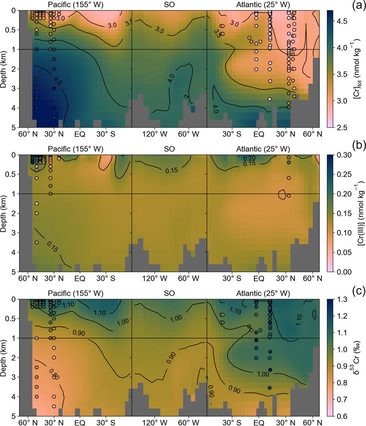
5450                                                                         F. Pöppelmeier et al.: Modeling the marine chromium cycle

Sun et al., 2019). Hence, we adopt a simplified parametriza-                   further shaped by the particle concentration and the particle
tion that is in general agreement with these estimates and the                 sinking velocity (v), which is considered globally uniform
overall chemical behavior of the scavenging-prone Cr(III) to                   and constant (1000 m yr−1 ). Particles reaching the seafloor
be removed by 80 % and the much more soluble Cr(VI) to                         are fully remineralized, while the associated Cr is removed
be removed only by 20 %. Since our riverine database covers                    from the model, ultimately balancing the source terms.
only rivers accounting for a fraction of the global discharge,
we uniformly scale all riverine fluxes by a factor (λri ) to com-              2.2.2      Internal cycling
pensate for the missing data. Arguably, this over represents
larger, well-studied rivers and thus skews the distribution of                 Reversible scavenging not only prescribes Cr removal at the
riverine Cr fluxes to the oceans, but such a simplification is                 seafloor but also modulates the redistribution of Cr within the
consistent with the intermediate complexity of the Bern3D                      water column. At shallow depths reversible scavenging acts
model. The riverine Cr fluxes per unit volume, V(θ , φ), thus                  as a net sink, contributing to reduce the dissolved Cr frac-
read                                                                           tion, while it works as a net source at greater depths where
                                                                             adsorbed Cr is released back into solution. The internal Cr
  Cr(III)                                         Cr(III)                      cycling is further influenced by redox reactions. A handful
Sri       (θ, φ) = Fri (θ, φ) · cri · αri · 1 − γri
                                                                               of studies investigated redox reactions and pathways in con-
             1                                                                 trolled laboratory experiments, aiming to determine reaction
· λri ·            ,                                                   (5)
          V (θ, φ)                                                             rate constants (e.g., Emerson et al., 1979; Pettine et al., 1998,
                                                                               2008). As a note of caution, these experiments were con-

 Cr(VI)                                                   Cr(VI)
Sri        (θ, φ) = Fri (θ, φ) · cri · (1 − αri ) · 1 − γri
                                                                               ducted with substantially higher reactant concentrations than
             1                                                                 typically observed in the modern ocean, and thus simple ex-
· λri ·            .                                                   (6)
          V (θ, φ)                                                             trapolations to mean ocean concentrations may not always be
                                                                               fully valid. We therefore consider these reaction rates only
Finally, the third major source of Cr in the model is a ben-                   as first-order approximations and further adjust them during
thic flux, Sbs (θ , φ), emanating from all sediment–water inter-               model tuning.
faces. Pore-water Cr data are limited (Brumsack and Gieskes,                      Divalent iron, Fe(II), which is produced by photochemi-
1983; Shaw et al., 1990), and currently, only one open ocean                   cal (e.g., Barbeau et al., 2001) and biological processes (e.g.,
pore-water [Cr] profile exists that quantifies the first-order                 Maldonado and Price, 2001) in surface waters, constitutes the
magnitude of the flux (Janssen et al., 2021). Hence, no                        main reductant for Cr (Pettine et al., 1998). In order to reflect
inferences on the spatial variability in this source can be                    these surface-specific processes in the model, Cr reduction is
made at this point. We therefore apply a globally uniform                      parameterized differently in the surface ocean compared to
parametrization for the benthic flux. Based on the pore-water                  the deep where photochemical and biologically mediated re-
investigations by Janssen et al. (2021), it is suggested that                  actions are strongly attenuated or likely absent. Thus, Cr(VI)
adsorbed Cr(III) is slowly oxidized back to soluble Cr(VI)                     reduction is increased in the uppermost grid cells by a fac-
in the pore water, which accumulates and ultimately escapes                    tor λsurf
                                                                                     reduc compared to the deep ocean, and a dependency on
from the sediment due to the build up of a concentration gra-                  POM export productivity, PPOM (θ ,φ), relative to its global
dient between bottom and pore waters. We therefore assume                      maximum is introduced. While reaction rates are dependent
that the majority (80 %) of the benthic Cr flux is in the form                 on the concentrations of the reactants, Fe(II) and other poten-
of Cr(VI), which leads to                                                      tial reductants are not explicitly implemented in the model.
                                     1                                         Chromium reduction in the model is thus solely controlled
 Cr(III)
Sbs        (θ, φ, z) = Fbs · αbs ·         ,                           (7)     by the Cr(VI) concentration as follows:
                               V (θ, φ, z)
                                                                                surf
 Cr(VI)                                    1                                   RVI→III (θ, φ) = kreduc · λsurf
                                                                                                          reduc · [Cr (VI)] (θ, φ)
Sbs     (θ, φ, z) = Fbs · (1 − αbs ) ·             ,                   (8)
                                       V (θ, φ, z)                                 PPOM (θ, φ)
                                                                               ·               ,                                            (9)
where αbs is the ratio of Cr(III) to Cr(VI) speciation.                            PPOM,MAX
   The sole sink of Cr considered in the model relates to
                                                                               where kreduc (yr−1 ) is the rate constant also used for the tun-
the removal and export of Cr with sinking particles. The re-
                                                                               ing, and for the deep ocean it is
versible scavenging scheme used in the Bern3D model is de-
scribed in detail by Rempfer et al. (2011) and follows pre-                        deep
                                                                               RVI→III (θ, φ, z) = kreduc · [Cr (VI)] (θ, φ, z) .          (10)
vious descriptions (Henderson et al., 1999; Marchal et al.,
2000). In brief, the scavenging efficiencies of Cr(III) and                    In the ocean interior, Cr reduction is also observed in oxy-
Cr(VI) to the four different particles types i (CaCO3 , POM,                   gen minimum zones (OMZs) (e.g., Cranston and Murray,
biogenic opal, lithogenics) are described by the particle affin-               1978; Huang et al., 2021; Murray, 1983; Rue et al., 1997),
ity coefficients Kdi . It is the magnitude of Kdi that determines              although data on reaction and removal rates (kOMZ ) remain
the solubility of the different ocean tracers. Removal rates are               very sparse. We include this specific process in the model

Biogeosciences, 18, 5447–5463, 2021                                                                 https://doi.org/10.5194/bg-18-5447-2021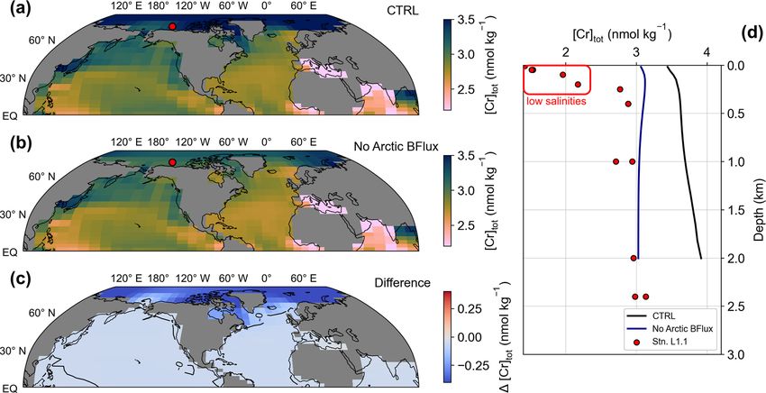
F. Pöppelmeier et al.: Modeling the marine chromium cycle                                                                          5451

and prescribe dissolved O2 concentrations < 5 µmol kg−1 as               Latin hypercube sampling approach, which significantly re-
the threshold (ηOMZ ) below which Cr reduction is strongly               duces the required number of simulations while maintaining
enhanced in the model (Moos et al., 2020; Nasemann et al.,               good coverage of the parameter space. In total, we performed
2020).                                                                   500 tuning simulations each integrated over 40 kyr. This was
                                                                        insufficient for all simulations to reach equilibrium. We in-
 OMZ                             1   for [O2 ] (θ, φ, z) ≤ ηOMZ          dividually examined this small subset of simulations which
RVI→III (θ, φ, z) = kOMZ ·       0               else             (11)
                                                                         had not yet reached equilibrium after 40 kyr and found unre-
On the other hand, Cr(III) is slowly oxidized back to Cr(VI)             alistically high Cr concentrations in all of them and therefore
for instance by H2 O2 (Pettine et al., 2008). Hydrogen perox-            did not continue model integration for these runs.
ide concentrations decrease with depth due to photochemi-                   The model performance was evaluated by determining the
cal production, atmospheric deposition to surface waters, and            mean absolute error (MAE) of the modern seawater data and
subsequent decomposition (Kieber et al., 2001). We there-                [Cr]tot of the closest model grid cell (root mean squared er-
fore additionally introduce a surface scaling for the oxidation          rors are noted in Table S3). For this, we compiled seawater
λsurf                                                                    measurements from the literature (n = 701, Table S2). Sea-
  oxid analogous to Eq. (9).
                                                                         water Cr concentrations have been determined since the late
 surf                                                                    1970s with increasing efforts in the past years and the recent
RIII→VI (θ, φ) = koxid · λsurf
                          oxid · [Cr (III)] (θ, φ)                (12)
                                                                         integration in the GEOTRACES initiative. Early seawater
 deep
RIII→VI (θ, φ, z) = koxid · [Cr (III)] (θ, φ, z)                  (13)   measurements were often performed using unfiltered sam-
                                                                         ples, which led to possible overestimation of dissolved Cr
Summing up all external sources into Stot (θ ,φ,z) and com-              due to particulate phases (Cranston, 1983). Yet, contamina-
bining the surface and deep ocean oxidation and reduction                tion during sample processing may also pose a potential issue
                      deep
equations Risurf and Ri    into Ri , the conservation equations          (e.g., see discussion in Nasemann et al., 2020). Therefore,
can be written as                                                        we performed a strict quality control and excluded all data
                                                                         for which such concerns were mentioned in the original pub-
∂ [Cr (III)]                                    OMZ                      lications, were identified in later studies, or exhibited incon-
             = Stot [Cr (III)]d + RVI→III + RVI→III
    ∂t                                                                   sistencies such as unrealistically large scatter within a depth

              ∂ v · Cr(III)p                                             profile (see Sect. S1). Finally, we excluded data from coastal
− RIII→VI −                        + T [Cr (III)] ,               (14)
                       ∂z                                                stations that were found to be affected by anthropogenic Cr
∂ [Cr (VI)]                                     OMZ
                                                                         loading (e.g., Hirata et al., 2000; Shiller and Boyle, 1987) or
             = Stot [Cr (VI)]d − RVI→III − RVI→III                       otherwise controlled by localized processes not represented
    ∂t
                                                                      by the resolution of the model, as well as studies in which
              ∂ v · Cr(VI)p
+ RIII→VI −                        + T [Cr (VI)] ,                (15)   quantitative comparisons to the model results are limited by
                       ∂z                                                poor analytical precision. The final global coverage of sea-
where subscripts d and p indicate the dissolved and particu-             water Cr measurements is biased towards the top 1000 m of
late phases, respectively, and T corresponds to the physical             the water column and the North Atlantic and North Pacific.
transport and mixing calculated in the model.
                                                                         2.3   Sensitivity experiments
2.2.3   Model tuning
                                                                         The Arctic Ocean experiences only limited water mass ex-
To date the marine Cr cycle remains largely under-                       change with the adjacent ocean basins via narrow straits. At
constrained, and hence a number of model parameters are                  the same time, it exhibits a high sediment surface-to-ocean
either unknown or estimated as first-order approximations.               volume ratio. Both these circumstances dramatically increase
We therefore tuned five different parameters, namely the ben-            the impact of a benthic flux on the regional tracer budget.
thic flux Fbs , the oxidation rate constant koxi (related to kreduc      Thus, in order to explore the relationship between the benthic
by a constant factor of 20, based on laboratory experiments;             flux and the mean Arctic Cr concentration, we conducted an
Elderfield, 1970; Pettine et al., 1998, 2008), the OMZ re-               idealized experiment in which we set the benthic flux of Cr
duction rate constant kOMZ , and reference scavenging pa-                to zero north of 70◦ N (simulation NoArcticBFlux).
rameters for Cr(III) and Cr(VI) (Table S1). The ratios of the               Further, due to data constraints, the model tuning was
affinities to the different particles were held constant and are         based solely on total Cr concentrations, yet the internal re-
noted in Table S2. The relatively long residence time of Cr in           dox cycling and the resulting distribution between Cr(III)
the ocean, estimated to range between 2 and 40 kyr (Camp-                and Cr(VI) are also of crucial importance for the potential
bell and Yeats, 1981; Sirinawin et al., 2000), requires model            applicability of Cr and its isotopes as a paleo-redox proxy.
integration times at least on the same order of magnitude.               To date, a relatively limited amount of information regard-
This makes a systematic exploration of the five-dimensional              ing open ocean Cr speciation is available, yet observations
tuning parameter space challenging. We therefore employ a                suggest widespread Cr reduction in OMZs below a thresh-

https://doi.org/10.5194/bg-18-5447-2021                                                         Biogeosciences, 18, 5447–5463, 2021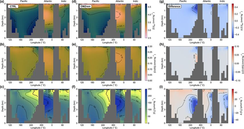
5452                                                              F. Pöppelmeier et al.: Modeling the marine chromium cycle

old O2 concentration (Goring-Harford et al., 2018; Huang
et al., 2021; Moos et al., 2020; Rue et al., 1997). In order
to explore the consequences of OMZ Cr reduction on the
global Cr inventory, we performed a number of idealized sen-
sitivity experiments. As noted in Sect. 2.1, in our standard
configuration POM remineralization is prescribed as a glob-
ally uniform power-law profile (Martin et al., 1987). Even
though total export fluxes are in good agreement with ob-
servations using such parametrization (Parekh et al., 2008),
the POM remineralization in OMZs is not adequately rep-
resented. Recently, Battaglia and Joos (2018) introduced a
new formulation in the Bern3D model that assigns POM
remineralization to aerobic or anaerobic pathways depend-
ing on the dissolved O2 concentration. Both are defined as
power-law profiles yet with different remineralization length
scales, yielding reduced remineralization rates under anaer-
obic conditions (see Battaglia Battaglia and Joos, 2018 for
details). We therefore performed a set of sensitivity experi-
ments in which we replaced the globally uniform POM rem-
ineralization with the improved parametrization introduced
by Battaglia and Joos (2018) (simulation OMZrem).
   In a third experiment, we investigated the impact of a
substantially stronger Cr reduction rate in OMZs as sug-
gested by field observations (Huang et al., 2021; Moos et
al., 2020; Rue et al., 1997). For this simulation we in-
creased the OMZ reduction rate from 4 nmol m−3 yr−1 in
the control run to 20 nmol m−3 yr−1 while also using the
improved two-pathway POM remineralization of Battaglia
and Joos (2018) (simulation OMZrem20). Finally, we per-
formed an experiment with an even higher reduction rate of          Figure 1. (a) Export fluxes of particulate organic matter (POM)
30 nmol m−3 yr−1 (OMZrem30). All these experiments were             and (b) biogenic opal calculated in the biogeochemical model from
branched off from the fully equilibrated control (CTRL) run         prognostic equations (Parekh et al., 2008). The distribution of cal-
under pre-industrial boundary conditions and are summa-             cium carbonate (CaCO3 ) production is the same as for POM but
rized in Table 2.                                                   scaled by the Redfield ratio and a Ca to P ratio of 0.3 in calci-
                                                                    fiers. (c) Log10 of the global dust flux estimated by Mahowald et
                                                                    al. (2006). The blue line indicates the transect for the section plots
                                                                    of Fig. 5.
3     Results

3.1    Constraints on benthic flux and residence time of
       Cr                                                           suggested a benthic flux of ∼ 3.2 nmol cm−2 yr−1 (Janssen et
                                                                    al., 2021). Overall, simulations with large benthic fluxes on
A wide array of estimates for the oceanic residence time of         the order of 1 nmol cm−2 yr−1 produce either Cr concentra-
Cr exists (defined as the total inventory divided by the sum        tions that are too high or unrealistically strong vertical gra-
of all source fluxes) ranging from 2 to 40 kyr (McClain and         dients (due to the large bottom source in combination with
Maher, 2016; Sirinawin et al., 2000; Wei et al., 2018). In          strong particle scavenging that is required under such con-
our parametrization, the mean ocean residence time of Cr is         ditions to balance the large benthic source flux). The clear
strongly influenced by the magnitude of the newly introduced        trend in the model–data misfit of the ensemble (Fig. 2a) in-
benthic flux representing the largest source in nearly all runs     dicates that reduced benthic fluxes are a fairly robust result
of the 500-member tuning ensemble. From this tuning en-             with the parametrization applied (i.e., globally uniform flux).
semble, we already obtain first constraints on the magnitude        Thus, we suspect that the benthic flux observed in the Tasman
of the benthic flux, as well as the mean ocean residence time       Basin may not be fully representative of the global ocean
of Cr, as both converge towards low MAEs (Fig. 2). In the           seafloor. However, missing processes in the internal cycling
ensemble, the best model–data agreement is achieved with            of the model that could be responsible for the mismatch can-
benthic fluxes in the range of 0.1 to 0.2 nmol cm−2 yr−1 , sub-     not be fully excluded at this point. Further, we note that we
stantially lower than the estimate from the Tasman Basin that       cannot distinguish whether the benthic Cr is of authigenic or

Biogeosciences, 18, 5447–5463, 2021                                                     https://doi.org/10.5194/bg-18-5447-2021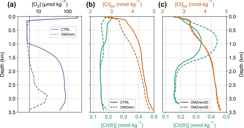
F. Pöppelmeier et al.: Modeling the marine chromium cycle                                                                              5453

Table 2. Different model simulations. Parameters not listed here were kept as in the control run (see Table 1). The mean absolute error (MAE)
was determined by comparing seawater observations to the model output at the closest grid cell.

                  Run                 POM                             OMZ reduction    Benthic                      MAE
                                      remineralization              (nmol m−3 yr−1 )   flux                   (nmol kg−1 )
                  CTRL                Martin et al. (1987)                        4    Globally uniform               0.48
                  NoArcticBFlux       Martin et al. (1987)                        4    Set to zero > 70◦ N            0.44
                  OMZrem              Battaglia and Joos (2018)                   4    Globally uniform               0.45
                  OMZrem20            Battaglia and Joos (2018)                  20    Globally uniform               0.45
                  OMZrem30            Battaglia and Joos (2018)                  30    Globally uniform               0.45

                                                                          servational data all exhibit Cr residence times between 5
                                                                          and 8 kyr (Fig. 2d). These relatively short residence times,
                                                                          compared to previous upper-limit estimates, are to some de-
                                                                          gree expected considering that benthic fluxes were either ne-
                                                                          glected or assumed to be fairly small in previous studies (e.g.,
                                                                          Reinhard et al., 2013) but are in contrast to the dominant Cr
                                                                          source in our model simulations. Yet, previous lower-limit
                                                                          estimates also did not include significant benthic sources but
                                                                          instead included anthropogenically contaminated rivers with
                                                                          exceedingly high Cr concentrations (e.g., the Panuco River;
                                                                          McClain and Maher, 2016), which are not considered here.

                                                                          3.2   Model–data comparison of the control run

                                                                          The tuning ensemble member that best fits the observational
                                                                          data of dissolved Cr concentrations (defined as the control
                                                                          run) yields an MAE of 0.48 nmol kg−1 . A few other simu-
                                                                          lations performed virtually as well as the control run, all of
                                                                          which exhibited similar values for the benthic flux and the
Figure 2. (a, c) Model performance of the tuning ensemble (cal-           scavenging factors. However, the parameters that describe
culated with the cost function of the mean absolute error, MAE –          the internal cycling (i.e., oxidation rate and OMZ reduction
the smaller the better) dependent on the benthic flux and (b, d) the      rate) exhibit a wider spread among these simulations. This is
diagnosed mean residence time of dissolved Cr. Note the logarith-
                                                                          related to the fact that our tuning target was solely the total
mic x axes in (a, b). (c, d) are zoom-ins of (a) and (b) and with
                                                                          Cr concentration, and we did not consider the individual ox-
linear x axes. Red ellipses indicate the simulations that best fit the
observational data.                                                       idation states in assessing model performance due to insuf-
                                                                          ficient data coverage to achieve statistical significance. The
                                                                          parameters of the control run are listed in Table 1.
                                                                             In the control run, the total flux of Cr entering the ocean
lithogenic origin in the model since we do not employ a sedi-             amounts to 8.77 × 10⁸ mol yr−1 with the smallest contri-
ment module for the calculation of the pore-water chemistry.              bution from dust (∼ 3 %), followed by the riverine source
It is thus possible that the benthic Cr is to some extent recy-           (∼ 29 %), and by far the largest contribution from the ben-
cled primary Cr from dust and rivers and not “new” Cr that                thic flux (∼ 68 %) (Table 1). Even though the global ben-
is added to the marine reservoir from the sediments. In that              thic flux of 0.16 nmol cm−2 yr−1 in the control run is much
case, the ocean residence time of Cr would increase propor-               smaller than the first local estimate (Janssen et al., 2021), it
tionally to the fraction of recycled Cr of the benthic source.            still dwarfs the combined contributions from dust and rivers.
As benthic sources account for approximately two-thirds of                In contrast, assuming both dust and river sources as in the
the total Cr source in our model (Table 1), this would yield              control run but a benthic flux comparable to the first local es-
a maximal increase of approximately a factor of 3 for our                 timate (∼ 3 nmol cm−2 yr−1 ) would yield a benthic flux con-
calculated residence times.                                               tribution of ∼ 98 % and be about 50 times larger than the
   The trend in the residence time versus model–data mis-                 riverine source. As previously noted by Janssen et al. (2021),
match is somewhat less distinct than that for the benthic flux            it thus appears that this first observational estimate for the
(Fig. 2b), but it still clearly converges towards the lower end           benthic flux from the Tasman Basin may not be fully repre-
of previous estimates. The simulations that best fit the ob-              sentative of the global ocean, and further research regarding

https://doi.org/10.5194/bg-18-5447-2021                                                           Biogeosciences, 18, 5447–5463, 2021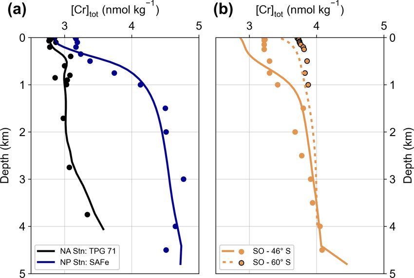
5454                                                                   F. Pöppelmeier et al.: Modeling the marine chromium cycle

                                                                         ern Australia (Rickli et al., 2019). In contrast, open ocean
                                                                         low- to mid-latitude surface Cr concentrations are slightly
                                                                         underestimated by the model compared to seawater data.
                                                                         The largest model–data discrepancy is observed in the Arc-
                                                                         tic Ocean where recent GEOTRACES data reveal remark-
                                                                         ably low surface Cr concentrations (Scheiderich et al., 2015),
                                                                         while simulated Cr concentrations are substantially higher
                                                                         (Figs. 4d; S1).
                                                                             These observed low surface Cr concentrations are accom-
                                                                         panied by low salinities indicating the influence of meltwater
                                                                         (Scheiderich et al., 2015). The exceptionally low trace metal
                                                                         concentrations in meltwater (due to the salt rejection during
                                                                         formation) may thus be responsible for the Arctic model–
                                                                         data discrepancy. Additionally, in the Bern3D model primary
                                                                         productivity is virtually absent in the Arctic mostly because
                                                                         the summer blooms restricted to coastal environments and
                                                                         near the sea-ice edge cannot be resolved in the model. Fur-
                                                                         ther, enhanced Cr reduction by Fe(II) that is released from
                                                                         the organic-rich Arctic shelf sediments is not explicitly im-
                                                                         plemented here. Thus, Arctic Cr removal by particle scaveng-
Figure 3. (a) Surface ocean total dissolved Cr concentration sim-
ulated in the control run. Filled circles mark surface seawater ob-
                                                                         ing remains extremely limited in the model. In combination
servations (top 40 m, equivalent to the height of the uppermost grid     with the sluggish exchange with the other ocean basins and
cell) with colors on the same scale as background model data. Cir-       the benthic flux constantly adding Cr, this produces elevated
cles with red edges are stations depicted in Fig. 6. (b) Same as (a)     Arctic Cr concentrations in the model. We therefore attribute
but for Cr(III) concentrations.                                          this inadequacy in simulating Arctic Cr to the simplifications
                                                                         in our description of the Cr cycle (e.g., the global uniform
                                                                         benthic flux, which may be substantially smaller in the Arc-
the impacts of sediment composition, porosity, and bottom                tic) and the relatively coarse resolution of the model. We test
and pore-water chemistry is required to better constrain this            the former attribution in a sensitivity experiment (simula-
presumably significant Cr source to the ocean.                           tion NoArcticBFlux) by setting the benthic flux to zero north
                                                                         of 70◦ N. Indeed, Arctic surface Cr concentrations are up to
3.2.1   Surface ocean                                                    0.5 nmol kg−1 lower in simulation NoArcticBFlux compared
                                                                         to CRTL (Fig. 4). This suggests that the benthic flux has sig-
The surface ocean [Cr]tot simulated in the control run re-               nificant impact even on surface concentrations in the semi-
veals a distinct meridional gradient with the highest values of          enclosed Arctic basin.
around 3.5 nmol kg−1 in the high latitudes decreasing equa-                  The surface distribution of Cr(III) (Fig. 3b) somewhat rep-
torwards (Fig. 3). The lowest surface [Cr]tot is simulated in            resents that of the POM export productivity (Fig. 1). This is
the high-productivity regions off the coast of East Africa and           related to our choice of parametrization that scales the sur-
the equatorial Indian Ocean, as well as in the Mediterranean             face Cr reduction rate with the POM export (see Sect. 2.2).
Sea. However, caution should be placed on the interpretation             However, differences are apparent as spatial variations are
of the simulated Cr concentrations in semi-enclosed basins               smaller for Cr(III) due to high removal rates by particle scav-
such as the Mediterranean Sea, which are poorly represented              enging in regions with high Cr reduction rates (i.e., high-
by the coarse spatial resolution of the model. Overall, Cr is            productivity regions).
more strongly reduced in upwelling regions, which together                   Seawater Cr(III) measurements are comparatively sparse,
with the high particle concentrations associated with high               and reported data are partly inconsistent presumably due to
primary productivity (Fig. 1) promotes efficient scaveng-                its high reactivity complicating sample processing, standard-
ing. Surface Cr concentrations are further impacted by large             ization, and intercalibration, as well as the lack of sample
river systems with high dissolved Cr concentrations such as              filtering in some studies (e.g., Connelly et al., 2006). Thus,
the Congo River, the Yangtze, or the Ganges–Brahmaputra,                 a model–data assessment is premature at the current stage.
which produce elevated concentrations at their river mouths.             Nevertheless, the North Pacific meridional gradient from the
   The comparison of the control run to observational Cr data            high-productivity region off the coast of Alaska to the olig-
in the uppermost 40 m (height of the surface grid cell) shows            otrophic subtropical gyre by Janssen et al. (2020) is fairly
good agreement overall. For instance, the strong meridional              well-represented in the control run. Yet, we reiterate that the
gradient in the Southern Ocean described above is also rep-              model tuning was not targeted at optimizing the Cr(III) dis-
resented in a meridional transect from Antarctica to south-              tribution, and a better representation of trivalent Cr in the

Biogeosciences, 18, 5447–5463, 2021                                                        https://doi.org/10.5194/bg-18-5447-2021
F. Pöppelmeier et al.: Modeling the marine chromium cycle 5455
Figure 4. (a–c) Surface total Cr concentrations for simulations CTRL and NoArcticBFlux, as well as the difference between both. The red
circle marks the location of station L1.1 of Scheiderich et al. (2015) depicted in (d). (d) [Cr]tot depth transect from the Arctic. Lines represent
model output of simulations CTRL (black) and NoArcticBFlux (blue) of the grid cells closest to station L1.1 (red circles).
model could most likely be achieved with a better coverage are underestimated as discussed above). Part of the Atlantic
of observational data and an improved understanding of the model–data mismatch might be attributed to the model sim-
Cr redox behavior in the ocean. ulating NADW that is too shallow due to deep water forma-
tion taking place too far south (Müller et al., 2006). Thus, the
3.2.2 Deep ocean extent of the low Cr concentration NADW endmember is un-
derestimated in the model. Further, as mentioned above, sim-
The distribution of simulated deep ocean total Cr concen- ulated Arctic [Cr]tot is far too high compared to observations.
trations is characterized by two pronounced and globally This regional model shortcoming is to some extent also prop-
consistent features (Figs. 5, 6). First is an increase in Cr agated into the Atlantic as Arctic water export through the
concentrations with depth that is smallest in the Southern Fram Strait contributes to the formation of NADW. In simu-
Ocean and northern North Atlantic (1[Cr]tot ≈ 1 nmol kg−1 ; lation NoArcticBFlux, in which the benthic flux is set to zero
top-to-bottom difference) and largest in the North Pacific at latitudes > 70◦ N, Arctic deep ocean Cr concentrations are
(1[Cr]tot > 2 nmol kg−1 ). The only exception to this feature up to 1 nmol kg−1 lower compared to CTRL (Fig. 4d), which
appears in the South Atlantic where Antarctic Intermediate indeed not only improves the model–data agreement in the
Water with fairly high total Cr concentrations overlays North Arctic but also in the North Atlantic (Table 2). Thus, simu-
Atlantic Deep Water (NADW), characterized by generally lated Atlantic Cr concentrations could be improved, for in-
lower dissolved Cr. The second feature relates to the accu- stance, by a revised representation of North Atlantic deep
mulation of Cr as water masses age, with the lowest con- water formation and a better understanding of regional dif-
centrations in waters dominated by newly formed NADW ferences in the benthic flux.
([Cr]tot ≈ 3 nmol kg−1 ) and gradually increasing towards the In a simplified approach we also converted the simu-
North Pacific where deep waters exhibit total Cr concentra- lated total Cr concentration to stable isotopic ratios based
tions > 4.5 nmol kg−1 (Fig. S3). Both these characteristics on the global oceanic array that exhibits a linear rela-
arise from the reversible scavenging scheme resulting in the tionship between δ 53 Cr and ln([Cr]tot ) (Fig. 5). Here we
net downward transport of Cr in combination with the ben- use δ 53 Cr = −0.70 · ln([Cr]tot ) + 1.86 based on Janssen et
thic flux gradually increasing bottom water Cr concentra- al. (2021). This also allows us to compare the model results
tions. to seawater isotopic ratios that are obtained independently
On a global scale, observational [Cr]tot data show very of the Cr concentrations. Overall, the model–data agreement
similar trends as simulated by the Bern3D model. Differ- for the isotopic ratios is comparable to [Cr]tot , indicating that
ences between the model and observations are mainly found deviations from the global array due to different fractiona-
in the Atlantic basin, where the model generally overesti- tion processes, as suggested for instance for OMZs (Moos et
mates total Cr concentrations (while surface concentrations al., 2020; Nasemann et al., 2020), have limited impact in the
https://doi.org/10.5194/bg-18-5447-2021 Biogeosciences, 18, 5447–5463, 20215456 F. Pöppelmeier et al.: Modeling the marine chromium cycle
Figure 5. (a) Total dissolved Cr concentrations along the transect marked in Fig. 1 from the North Pacific via the Southern Ocean (SO) to
the North Atlantic. Filled circles are seawater observations on the same color scale as the model data. (b) Dissolved Cr(III) distribution along
the same transect as in (a). (c) Calculated δ 53 Cr distribution based on the global ocean array assuming δ 53 Cr = −0.70 · ln([Cr]tot ) + 1.86
(Janssen et al., 2021) compared to observational isotope ratio data. Only observational seawater data close to the transect (±15◦ ) are shown.
Note the different y scales for the top 1 km.
open ocean. The Cr model implementation employed here 3.3 Improving the representation of Cr reduction in
thus holds the promise of also being applicable to investiga- OMZs
tions of sedimentary Cr stable isotopic data.
In contrast to the fairly variable surface Cr(III) concen-
trations, its distribution below a water depth of 500 m ex- Oxygen minimum zones are thought to represent important
hibits remarkable homogeneous values between 0.10 and environments where Cr is removed from the ocean and de-
0.15 nmol kg−1 throughout most of the well-oxygenated posited in the underlying sediments (Moos et al., 2020; Rue
global deep ocean (Fig. 5). Yet, reliable seawater data of et al., 1997) as they promote the reduction of soluble Cr(VI)
open ocean [Cr(III)] are too sparse for a reasonable global- to scavenging-prone Cr(III). In the model, about one-fourth
scale model–data comparison, and hence these model results of the entire Cr removal (calculated from the particulate con-
should be taken cautiously. centrations of the bottommost grid cells) takes place at the
sediments below OMZs (representing an area of 7.37 % of
the seafloor; Table 3). Yet, the simulated Cr(III) concentra-
tions of ∼ 0.15 nmol kg−1 are partly in disagreement with ob-
served Cr(III) concentrations in OMZs that can even exceed
1 nmol kg−1 (Huang et al., 2021; Moos et al., 2020; Rue et
Biogeosciences, 18, 5447–5463, 2021 https://doi.org/10.5194/bg-18-5447-2021F. Pöppelmeier et al.: Modeling the marine chromium cycle 5457
Table 3. OMZ volumes and sediment area below OMZs, as well as fraction of total Cr burial flux below OMZs. See Table 2 for more specific
information on the experiments.
Run Total (relative) volume Area fraction Sink fraction Sink fraction/
OMZ (106 km3 ) ([O2 ] ≤ 5 µmol kg−1 ) ([O2 ] < 5 µmol kg−1 ) area fraction
CTRL 12.6 (0.93 %) 7.37 % 24.84 % 3.37
OMZrem 10.2 (0.75 %) 3.87 % 15.63 % 4.04
OMZrem20 10.2 (0.75 %) 3.87 % 16.76 % 4.33
OMZrem30 10.2 (0.75 %) 3.87 % 17.46 % 4.51
issue with Earth system models of various complexity and is
mostly related to insufficient spatial resolution to adequately
represent these highly dynamic regions even with consider-
ably better spatially resolved models (Cocco et al., 2013).
The greater vertical extent and the strongly attenuated par-
ticle remineralization in the OMZs associated with the O2 -
dependent parametrization has a profound impact on the ver-
tical [Cr(III)] and [Cr]tot profiles (illustrated for the eastern
equatorial Pacific OMZ in Fig. 7b). In the upper part of the
OMZ, Cr(III) concentrations are lower compared to CTRL
due to the higher particle concentrations enhancing the scav-
enging efficiency. In contrast, in the lower part (below 1 km)
the effect of the deepened OMZ promoting Cr reduction
(local Cr(III) source) dominates over the elevated particle
concentrations associated with the vertical expansion (local
Figure 6. Comparisons between measured total Cr concentrations
Cr(III) sink). Both the elevated particle concentration in gen-
of four seawater stations (circles) and simulated values of the con-
trol run at the closest model grid cells (lines). North Atlantic station eral and the greater vertical extent of the OMZ increasing Cr
TPG 71 (Jeandel and Minster, 1987), North Pacific station SAFe reduction (integrated over the entire water column) lead to a
(Moos and Boyle, 2019), and Southern Ocean stations at 46◦ S decrease in total Cr concentration throughout the water col-
(composite of IN2018V04 – Stn. PS2, Janssen et al., 2021, and ACE umn, yet this effect is most pronounced in the depth range of
Leg2 – Stn. 8, Rickli et al., 2019) and 60◦ S (ACE Leg2 – Stn. 10, the OMZ.
Rickli et al., 2019). Nevertheless, Cr(III) concentrations also remain lower
in simulation OMZrem than observations of OMZs indi-
cate (of up to 1 nmol kg−1 ; Huang et al., 2021). We there-
fore performed two additional sensitivity experiments with
al., 1997). We consider this to be the result of the model tun- substantially increased OMZ reduction rates of 20 and
ing not taking into account the spatial distribution of Cr(III) 30 nmol m−3 yr−1 (simulations OMZrem20, OMZrem30, re-
due to the insufficient data coverage. Generally, modeled spectively) (compared to 4 nmol m−3 yr−1 in CTRL), in-
Cr(III) concentrations are only slightly elevated in OMZs cluding the parametrization of O2 -dependent remineraliza-
(Fig. 7b) in contrast to observations that suggest strong re- tion (Fig. 7c). For both these simulations, Cr(III) concentra-
duction rates and subsequent removal of Cr (e.g., Rue et al., tions are strongly elevated in OMZs, for instance, peaking at
1997). 0.33 and 0.44 nmol kg−1 in the core of the eastern equatorial
In a first sensitivity experiment (OMZrem) we therefore Pacific OMZ for OMZrem20 and OMZrem30, respectively,
replaced the globally uniform POM remineralization pro- compared to a maximum of ∼ 0.20 nmol kg−1 in CTRL. At
file with the O2 -dependent parametrization introduced by the same time, the effect of increased OMZ Cr reduction on
Battaglia and Joos (2018) (see Sect. 2.3). This reduces [Cr]tot within OMZs is relatively small with a minor decrease
the horizontal expansion of OMZs in the model but at in concentrations in the top 1 km and only slightly higher
the same time increases their vertical extent (see Fig. 7a). concentrations below. This redistribution in the water column
Consequently, the difference in ocean volume where [O2 ] is a direct consequence of the higher Cr(III) concentrations
< 5 µmol kg−1 is relatively moderate with a decrease from enhancing Cr downward transport and ultimately also re-
0.93 % in CTRL to 0.75 % of the total volume with the O2 - moval. Globally this results in 7 % and 12 % more Cr removal
dependent remineralization (Fig. 8). However, this is still an below OMZs for simulations OMZrem20 and OMZrem30,
overestimation of the modern expansion of OMZs by a fac- respectively, compared to OMZrem (Table 3). As such, the
tor of about 5 (see Bianchi et al., 2012). This is a persistent
https://doi.org/10.5194/bg-18-5447-2021 Biogeosciences, 18, 5447–5463, 20215458 F. Pöppelmeier et al.: Modeling the marine chromium cycle Figure 7. Eastern equatorial Pacific (7.5◦ N, 90◦ W) (a) oxygen concentration for CTRL (i.e., globally uniform POM remineralization) and the O2 -dependent remineralization as described by Battaglia et al. (2018) used for the sensitivity experiments. (b) Total Cr and Cr(III) concentrations for CTRL and simulation OMZrem. (c) Same as (b) but for simulations OMZrem20 and OMZrem30. Figure 8. Total Cr (a, d, g), Cr(III) (b, e, h), and O2 concentrations (c, f, i) along an east–west section at the Equator for the control run (a–c), simulation OMZrem (d–f), and the difference between both (OMZrem minus CTRL) (g–i). higher OMZ reduction rates, together with the O2 -dependent as simulated here. Thus, additional processes such as organic remineralization, do indeed provide an improved represen- complexation, which stabilizes Cr(III), or elevated Cr reduc- tation of OMZ Cr concentration characteristics (Cr(III) and tion at shallow depths might be at play in OMZs that are not Crtot ) consistent with observations (see Moos et al., 2020; explicitly implemented here. Rue et al., 1997). However, it is worthy of note that observa- tions indicate that the Cr(III) maximum in OMZ depth pro- files is shifted toward shallower depths (Huang et al., 2021; Rue et al., 1997) and not in the middle or bottom of the OMZ Biogeosciences, 18, 5447–5463, 2021 https://doi.org/10.5194/bg-18-5447-2021
F. Pöppelmeier et al.: Modeling the marine chromium cycle                                                                    5459

4     Discussion and conclusions                                   4.2   Limitations in simulating the marine Cr cycle

4.1    Global- and regional-scale performance                      The fairly long mean ocean residence time of Cr puts seri-
                                                                   ous constraints on its implementation in Earth system mod-
This study describes the first implementation of the modern        els. In order to obtain an equilibrated state of the marine
marine Cr cycle and more specifically of the two oxidation         Cr cycle, model integrations of several tens of thousands of
states, Cr(III) and Cr(VI), into an EMIC. We implemented           years are required. This can currently only be achieved with
three Cr sources, namely an aeolian, a riverine, and a ben-        highly computationally efficient, coarse-resolution, interme-
thic flux, that are balanced by the removal associated with        diate complexity models such as Bern3D. At the same time
reversible scavenging transferring particulate Cr to the sedi-     this limits the representation of the Cr cycle as small-scale
ment. The comparison of our 500-member tuning ensemble             processes, for instance at coastal regions, can inherently only
to a comprehensive and quality-controlled seawater database        be approximated in these models. Furthermore, because of
provides a best estimate for the mean ocean Cr residence           the scarcity of data, processes such as redox reactions, par-
time between 5 and 8 kyr, which is at the lower end of pre-        ticle scavenging, and sedimentary release of Cr remain criti-
vious first-order approximations (Campbell and Yeats, 1984;        cally under-constrained to date, which contributes to substan-
Reinhard et al., 2013; Wang et al., 2020). At the same time,       tial uncertainty in the understanding of the marine Cr cycle
we find that the best model–data agreement is achieved with        and thus also impedes its robust implementation in models.
benthic fluxes in the order of 0.1 to 0.2 nmol cm−2 yr−1 , sub-    As a consequence, only large-scale features of the Cr distri-
stantially lower than the first local estimates (Janssen et al.,   butions presented here can be considered as robust. Future
2021). Nevertheless, a benthic flux of such magnitude is sub-      improvements in the understanding of, for example, the spa-
stantially larger than the aeolian and riverine source fluxes      tial variability in the benthic flux or the Cr behavior in OMZs,
(for the control run: 68 % benthic, 29 % riverine, and 3 % ae-     might however bolster our ability to also simulate regional
olian).                                                            variations in better agreement with observations.
   Overall, the control run simulates the vertical, meridional,       One such more local, yet important, model–data discrep-
and inter-basin [Cr]tot gradients in good agreement with ob-       ancy relates to the simulated surface depletion of [Cr]tot that
servational data. Thus, total Cr concentrations increase with      is most pronounced above OMZs but not observed to the
depth, as well as with water mass age, which leads to [Cr]tot      same extent in existing seawater profiles (see Figs. 6 and 7;
> 4.5 nmol kg−1 in the deep North Pacific. Similarly, the ver-     Goring-Harford et al., 2018; Moos et al., 2020; Nasemann et
tical gradient increases from 1[Cr]tot ≈ 1 nmol kg−1 in the        al., 2020). The reversible scavenging scheme linearly scales
North Atlantic to 1[Cr]tot > 2.5 nmol kg−1 in the North Pa-        with the particle concentration. From this follows that Cr re-
cific. The only major model–data mismatch is observed in           moval is strongest in the surface ocean where no remineral-
the Arctic Ocean basin where simulated concentrations are          ization takes place in the model (euphotic zone) and in high-
far too high compared to observations. We attribute this to the    productivity regions that are also responsible for OMZs. One
poor spatial representation due to the coarse model resolution     possible explanation to account for the high particle concen-
and to the simplified benthic flux parametrization causing it      trations in these regions not leading to strong surface Cr de-
to have an impact that is too large on this semi-enclosed basin    pletions in the real ocean could relate to complexation with
with a large sediment surface area compared to its volume.         organic ligands. Complexation has been found to be an im-
   In contrast, the poor spatial data coverage of Cr(III) ob-      portant process increasing the solubility of a number of trace
servations precludes not only its incorporation in the tuning      metals such as rare earth elements (Byrne and Kim, 1990),
metric but also a robust model–data assessment that can only       Cu, Zn, Cd, and most notably Fe (Bruland and Lohan, 2003).
be improved by more seawater measurements. The only ex-            Similarly, investigations showed that Cr(III) readily binds
ception are OMZs that are fairly well-studied with respect to      with organic ligands (Saad et al., 2017), in contrast to Cr(VI),
Cr reduction and hence Cr(III) concentrations (e.g., Huang         which seems to be far less affected by complexation (Richard
et al., 2021; Moos et al., 2020; Murray et al., 1983; Rue et       and Bourg, 1991). The dominance of Cr(VI) in oxygenated
al., 1997). Yet, as a consequence of not including Cr(III) in      water therefore indicates that this process is unable to fully
the tuning metric, its representation in OMZs is somewhat          explain the simulated surface Cr depletion. Instead, we spec-
deficient. We therefore performed three sensitivity experi-        ulate that internal recycling processes in the mixed layer,
ments to improve simulated Cr(III) concentrations in these         not considered in our reversible scavenging parametrization,
highly reducing regions. By introducing an O2 -dependent           might be responsible for the observed relatively stable Cr
parametrization of POM remineralization and a strongly in-         concentrations in the uppermost water column. This could
creased OMZ reduction rate, we are able to simulate high           also explain the depleted surface concentrations of other geo-
Cr(III) concentrations and elevated Crtot removal in OMZs          chemical tracers implemented in the Bern3D model that also
that are in much improved agreement with observational             make use of the same reversible scavenging formulation (Nd:
data.                                                              Pöppelmeier et al., 2020; Pa: Rempfer et al., 2017).

https://doi.org/10.5194/bg-18-5447-2021                                                   Biogeosciences, 18, 5447–5463, 2021
You can also read