Effective radiative forcing from emissions of reactive gases and aerosols - a multi-model comparison - ACP
←
→
Page content transcription
If your browser does not render page correctly, please read the page content below
Atmos. Chem. Phys., 21, 853–874, 2021
https://doi.org/10.5194/acp-21-853-2021
© Author(s) 2021. This work is distributed under
the Creative Commons Attribution 4.0 License.

Effective radiative forcing from emissions of reactive gases and
aerosols – a multi-model comparison
Gillian D. Thornhill1 , William J. Collins1 , Ryan J. Kramer2,19 , Dirk Olivié3 , Ragnhild B. Skeie4 , Fiona M. O’Connor5 ,
Nathan Luke Abraham6,7 , Ramiro Checa-Garcia8 , Susanne E. Bauer9 , Makoto Deushi10 , Louisa K. Emmons11 ,
Piers M. Forster12 , Larry W. Horowitz13 , Ben Johnson5 , James Keeble7 , Jean-Francois Lamarque11 ,
Martine Michou14 , Michael J. Mills11 , Jane P. Mulcahy5 , Gunnar Myhre4 , Pierre Nabat14 , Vaishali Naik13 ,
Naga Oshima10 , Michael Schulz3 , Christopher J. Smith12,18 , Toshihiko Takemura15 , Simone Tilmes11 , Tongwen Wu16 ,
Guang Zeng17 , and Jie Zhang16
1 Department  of Meteorology, University of Reading, Reading, RG6 6BB, UK
2 Climate  and Radiation Laboratory, NASA Goddard Space Flight Center, Greenbelt, MD 20771, USA
3 Norwegian Meteorological Institute, Oslo, Norway
4 CICERO – Centre for International Climate and Environmental Research Oslo, Oslo, Norway
5 Met Office, Exeter, UK
6 National Centre for Atmospheric Science, University of Cambridge, Cambridge, UK
7 Department of Chemistry, University of Cambridge, Lensfield Road, Cambridge, CB2 1EW, UK
8 Laboratoire des Sciences du Climat et de l’Environnement, IPSL/CNRS, 91191 Gif-sur-Yvette, France
9 NASA Goddard Institute for Space Studies, New York, NY 10025, USA
10 Meteorological Research Institute, Tsukuba, Japan
11 National Center for Atmospheric Research, Boulder, CO 80307-3000, USA
12 School of Earth and Environment, University of Leeds, LS2 9JT, UK
13 NOAA, Geophysical Fluid Dynamics Laboratory (GFDL), Princeton, NJ 08540-6649, USA
14 CNRM, Université de Toulouse, Météo-France, CNRS, Toulouse, France
15 Research Institute for Applied Mechanics, Kyushu University, Kasuga, Fukuoka, Japan
16 Climate System Modeling Division, Beijing Climate Center, Beijing, China
17 National Institute of Water and Atmospheric Research (NIWA), Wellington, New Zealand
18 International Institute for Applied Systems Analysis (IIASA), Laxenburg, Austria
19 Universities Space Research Association, 7178 Columbia Gateway Drive, Columbia, MD 21046, USA

Correspondence: Gillian D. Thornhill (g.thornhill@reading.ac.uk)

Received: 29 December 2019 – Discussion started: 13 March 2020
Revised: 20 October 2020 – Accepted: 31 October 2020 – Published: 21 January 2021

Abstract. This paper quantifies the pre-industrial (1850) to    methane. Where possible we break down the ERFs from each
present-day (2014) effective radiative forcing (ERF) of an-     emitted species into the contributions from the composition
thropogenic emissions of NOX , volatile organic compounds       changes. The ERFs are calculated for each of the models that
(VOCs; including CO), SO2 , NH3 , black carbon, organic         participated in the AerChemMIP experiments as part of the
carbon, and concentrations of methane, N2 O and ozone-          CMIP6 project, where the relevant model output was avail-
depleting halocarbons, using CMIP6 models. Concentration        able.
and emission changes of reactive species can cause multi-         The 1850 to 2014 multi-model mean ERFs (± stan-
ple changes in the composition of radiatively active species:   dard deviations) are −1.03 ± 0.37 W m−2 for SO2
tropospheric ozone, stratospheric ozone, stratospheric wa-      emissions, −0.25 ± 0.09 W m−2 for organic carbon
ter vapour, secondary inorganic and organic aerosol, and        (OC), 0.15 ± 0.17 W m−2 for black carbon (BC) and

Published by Copernicus Publications on behalf of the European Geosciences Union.
854                        G. D. Thornhill et al.: Effective radiative forcing from emissions of reactive gases and aerosols

−0.07 ± 0.01 W m−2 for NH3 . For the combined aerosols            tive forcing (Forster et al., 2016; Sherwood et al., 2015),
(in the piClim-aer experiment) it is −1.01 ± 0.25 W m−2 .         which generally considered the instantaneous radiative forc-
The multi-model means for the reactive well-mixed                 ing (IRF), or a combination of the IRF including the adjust-
greenhouse gases (including any effects on ozone and              ment of the stratospheric temperature to the driver, gener-
aerosol chemistry) are 0.67 ± 0.17 W m−2 for methane              ally termed the stratospheric-temperature-adjusted radiative
(CH4 ), 0.26 ± 0.07 W m−2 for nitrous oxide (N2 O) and            forcing. More recently (Boucher, 2013; Chung and Soden,
0.12 ± 0.2 W m−2 for ozone-depleting halocarbons (HC).            2015) there has been a move towards using the effective ra-
Emissions of the ozone precursors nitrogen oxides (NOx ),         diative forcing (ERF) as the preferred metric, as this includes
volatile organic compounds and both together (O3 ) lead to        the rapid adjustments of the atmosphere to the perturbation,
ERFs of 0.14 ± 0.13, 0.09 ± 0.14 and 0.20 ± 0.07 W m−2            e.g. changes in cloud cover or type, water vapour, and tro-
respectively. The differences in ERFs calculated for the          pospheric temperature, which may affect the overall radia-
different models reflect differences in the complexity of         tive balance of the atmosphere. In this work, ERF is calcu-
their aerosol and chemistry schemes, especially in the case       lated using two atmospheric model simulations, both with
of methane where tropospheric chemistry captures increased        the same prescribed sea surface temperatures (SSTs) and sea
forcing from ozone production.                                    ice, but with one having the perturbation we are interested in
                                                                  investigating, e.g. a change in emissions or concentrations of
                                                                  aerosols or reactive gases. The difference in the net TOA flux
                                                                  between these two simulations is then defined as the ERF for
1   Introduction                                                  that perturbation.
                                                                     Previous efforts to understand the radiative forcing due
The characterization of the responses of the atmosphere, cli-     to aerosols and reactive gases in CMIP simulations have re-
mate and Earth systems to various forcing agents is essen-        sulted in a wide spread of values from the different climate
tial for understanding, and countering, the impacts of cli-       models, in part due to a lack of suitable model simulations
mate change. As part of this effort there have been sev-          for extracting the ERF from for example a specific change
eral projects directed at using climate models from different     to an aerosol species. The experiments in the AerChemMIP
groups around the world to produce a systematic compari-          project have been designed to address this in part by defining
son of the simulations from these models, via the Coupled         consistent model set-ups to be used to calculate the ERFs, al-
Model Intercomparison Project (CMIP), which is now in its         though the individual models will still have their own aerosol
sixth iteration (Eyring et al., 2016). This CMIP work has         and chemistry modules, with varying levels of complexity
been subdivided into different areas of interest for addressing   and different approaches.
specific questions about climate change, such as the impact          There are complexities in assessing how a particular forc-
of aerosols and reactive greenhouse gases, and the AerChem-       ing agent affects the climate system due to the interactions
MIP (Collins et al., 2017) project is designed to examine the     between some of the reactive gases; for example methane
specific effects of these factors on the climate. The aerosol     and ozone are linked in complex ways, and this increases the
and aerosol precursor species considered are sulfur dioxide       problem of understanding the specific contribution of each
(SO2 ), black carbon (BC) and organic carbon (OC). The re-        to the overall ERFs when one of them is perturbed. An at-
active greenhouse gases and ozone precursors are methane          tempt to understand some of these interactions is discussed
(CH4 ), nitrogen oxide (NOX ), volatile organic compounds         in Sect. 4.2 below.
(VOCs – including carbon monoxide), nitrous oxide (N2 O)             The experimental set-up and models used are described in
and ozone-depleting halocarbons (HC).                             Sect. 2, the methods for calculating the ERFs for the aerosol
   The focus of this work is to characterize the effect of the    and chemistry experiments are described in Sect. 3, and the
change from pre-industrial (1850) to present day (2014) in        results are discussed in Sect. 4. Final conclusions are drawn
aerosols and their precursors, as well as the effect of chemi-    in Sect. 5.
cally reactive greenhouse gases (including species that affect
ozone) on the radiation budget of the planet, referred to as
radiative forcing, as an initial step to understanding the re-    2     Experimental set-up
sponse of the atmosphere and Earth system to changes in
these components. In previous reports of the Intergovern-         2.1    Models
mental Panel on Climate Change (IPCC) the effect of the
various forcing agents on the radiation balance has been          This analysis is based on models participating in the Cou-
investigated in terms of the radiative forcing (RF), which        pled Model Intercomparison Project (CMIP6) (Eyring et al.,
is a measure of how the radiative fluxes at the top of the        2016), which oversees climate modelling efforts from a num-
atmosphere (TOA) change in response to changes in for             ber of centres with a view to facilitating comparisons of the
example concentrations or emissions of greenhouse gases           model results in a systematic framework. The overall CMIP6
and aerosols. There have been several definitions of radia-       project has a number of sub-projects, where those with in-

Atmos. Chem. Phys., 21, 853–874, 2021                                                https://doi.org/10.5194/acp-21-853-2021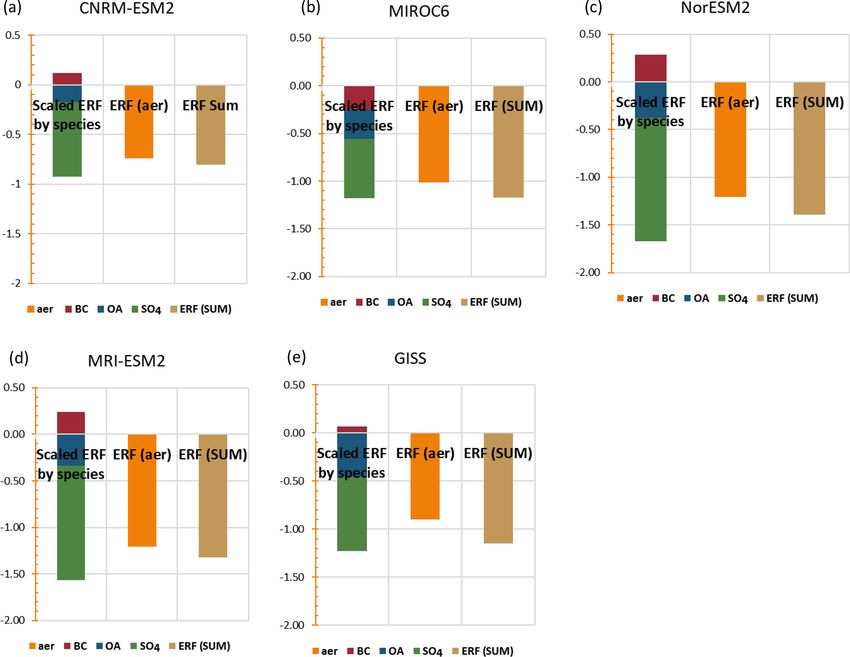
G. D. Thornhill et al.: Effective radiative forcing from emissions of reactive gases and aerosols                            855

terests in specific aspects of the climate can design and re-      and a chemistry model, MRI-CCM2 (Deushi and Shibata,
quest specific experiments to be undertaken by the modelling       2011), which models chemistry processes for ozone and
groups. To understand the effects of aerosols and reactive         other trace gases from the surface to middle atmosphere. The
gases on the climate, a set of experiments was devised un-         model includes aerosol–chemistry interactions and aerosol–
der the auspices of AerChemMIP (Collins et al., 2017), de-         cloud interactions (Kawai et al., 2019). The ERFs of anthro-
scribed in Sect. 2.2.                                              pogenic gases and aerosols under present-day conditions rel-
   The anthropogenic emissions of the aerosols, aerosol pre-       ative to pre-industrial conditions estimated by MRI-ESM2 as
cursors and ozone precursors (excluding methane) for use in        part of the Radiative Forcing Model Intercomparison Project
the models are given by Hoesly et al. (2018) and van Marle         (RFMIP) (Pincus et al., 2016) and AerChemMIP are summa-
et al. (2017). Models use their own natural emissions (Eyring      rized in Oshima et al. (2020).
et al., 2016). The well-mixed greenhouse gases (WMGHG),               The BCC-ESM1 model (Wu et al., 2019, 2020) models
CO2 , CH4 , N2 O and halocarbons, are specified as concen-         major aerosol species including gas-phase chemical reactions
trations either at the surface or in the troposphere. Not all of   and secondary aerosol formation, and aerosol–cloud interac-
the models include interactive aerosols, tropospheric chem-        tions including indirect effects are represented. It does not
istry and stratospheric chemistry, which is the ideal for the      include stratospheric chemistry, so concentrations of ozone,
AerChemMIP experiments, but those models which do not              CH4 and N2 O at the top two model levels are the zonally and
include all these processes provide results for a subset of the    monthly values derived from the CMIP6 data package.
experiments described in Sect. 2.2.                                   The NorESM2 model contains interactive aerosols and
   The models included in this analysis are summarized be-         uses the OsloAero6 aerosol module (Seland et al., 2020),
low, and in Table 1 with an overview of the model set-up,          which describes the formation and evolution of BC, OC,
aerosol scheme and type of chemistry models used included.         SO4 , dust, sea salt and SOA. There is a limited gas-phase
A more detailed description of each model and the aerosol          chemistry describing the oxidation of the aerosol precur-
and chemistry schemes used in each is available in the Sup-        sors DMS, SO2 , isoprene and monoterpenes; oxidant fields
plement, Table S1.                                                 of OH, HO2 , NO3 and ozone are prescribed climatological
   The CNRM-ESM2-1 model (Séférian et al., 2019; Mi-               fields; and there is no ozone chemistry in the model.
chou et al., 2020) includes an interactive tropospheric aerosol       The GFDL-ESM4 model consists of the GFDL AM4.1
scheme and an interactive gaseous chemistry scheme only            atmosphere component (Dunne et al., 2020; Horowitz et
above the level of 560 hPa. The sulfate precursors evolve          al., 2020), which includes an interactive tropospheric and
to SO4 using a simple dependence on latitude. The cloud            stratospheric gas-phase and aerosol chemistry scheme. Ni-
droplet number concentration (CDNC) depends on SO4 , or-           trate aerosols are explicitly treated in this model.
ganic matter and sea salt concentrations, so the aerosol cloud        The CESM2-WACCM model includes interactive chem-
albedo effect is represented, although other aerosol–cloud in-     istry and aerosols for the troposphere, stratosphere and lower
teractions are not.                                                thermosphere (Emmons et al., 2010); (Gettelman et al.,
   The UKESM1 model (Sellar et al., 2020) includes an inter-       2019). The representation of secondary organic aerosols fol-
active stratosphere–troposphere gas-phase chemistry scheme         lows the volatility basis set approach (Tilmes et al., 2019).
(Archibald et al., 2020) using the UK Chemistry and Aerosol           The IPSLCM6A-LR-INCA (referred to subsequently as
(UKCA; Morgenstern et al., 2009; O’Connor et al., 2014)            IPSL-INCA) model used for this analysis has interactive
model. The UKCA aerosol scheme, called GLOMAP mode                 aerosols but a limited gas-phase model. The aerosol scheme
is two-moment simulation of tropospheric black carbon, or-         is based on a sectional approach to represent the size distri-
ganic carbon, SO4 and sea salt. Dust is modelled inde-             bution of dust, sea salt (which has an additional super-coarse
pendently using the bin scheme of Woodward (2001). A               mode to model largest emission of spray-salt aerosols), BC,
full description and evaluation of the chemistry and aerosol       NH4 , NO3 , SO4 , SO2 and organic aerosol (OA) with a com-
schemes in UKESM1 can be found in Archibald et al. (2020)          bination of accumulation and coarse log-normal modes with
and Mulcahy et al. (2020) respectively.                            both soluble and insoluble treated as independent modes.
   The MIROC6 model includes the Spectral Radiation-               DMS emissions are prescribed and not interactively cal-
Transport Model for Aerosol Species (SPRINTARS) aerosol            culated. BC is modelled as internally mixed with sulfate
model, which predicts mass mixing ratios of the main tro-          (Wang et al., 2016), where the refractive index relies on
pospheric aerosols and models aerosol–cloud interactions in        the Maxwell-Garnett method. Its emissions are derived from
which aerosols alter cloud microphysical properties and af-        inventories. A new dust refractive index is implemented
fect the radiation budget by acting as cloud condensation          (Di Biagio et al., 2019). Well-mixed trace gas concentra-
and ice nuclei (Takemura et al., 2005, 2018; Watanabe et al.,      tions/emissions are forced with AMIP/CMIP6 datasets (Lur-
2010; Takemura and Suzuki, 2019; Tatebe et al., 2019).             ton et al., 2020), ozone using Checa-Garcia et al. (2018) and
   The MRI-ESM2 model (Yukimoto et al., 2019) has the              solar forcing from Matthes et al. (2017).
Model of Aerosol Species in the Global Atmosphere mark-               The GISS-E2-1 model aerosol scheme (one-moment
2 revision-4 climate (MASINGAR mk-2r4c) aerosol model,             aerosol, OMA) module, which includes sulfate, nitrate, am-

https://doi.org/10.5194/acp-21-853-2021                                               Atmos. Chem. Phys., 21, 853–874, 2021
856                         G. D. Thornhill et al.: Effective radiative forcing from emissions of reactive gases and aerosols

Table 1. Components used in the Earth system models (a detailed table is in the Supplement, Table S1).

                                  Aerosols                           Tropospheric chemistry                 Stratospheric chemistry
       IPSL-CM6A-LR-INCA          Interactive                        No                                     No
       NorESM2-LM                 Interactive                        SOA and sulfate precursor chemistry    No
       UKESM1-LL                  Interactive tropospheric           Interactive                            Interactive
                                  Prescribed stratospheric
       CNRM-ESM2-1                Interactive                        Chemical reactions down to 560 hPa     Interactive
       MRI-ESM2                   Interactive                        Interactive                            Interactive
       MIROC6                     Interactive                        SOA and sulfate precursor chemistry    No
       BCC-ESM1                   Interactive                        Interactive                            No
       GFDL-ESM4                  Interactive                        Interactive                            Interactive
       CESM2-WACCM                Interactive                        Interactive                            Interactive
       GISS-E2-1                  Interactive                        Interactive                            Interactive

monium and carbonaceous aerosols (BC and OC), is coupled                  vidually or in groups. This provides ERFs for the specific
to both the tropospheric and stratospheric chemistry scheme.              emission or concentration change but also for all aerosol pre-
For the results reported here, the physics version 3 of this              cursor or NTCFs combined (Collins et al., 2017). For mod-
model configuration was used, which includes the aerosol                  els without interactive tropospheric chemistry “NTCF” and
impacts on clouds. For details of the model, see Bauer et                 “aer” experiments are the same; in the case of NorESM2 for
al. (2020).                                                               the NTCF experiments the model attempts to mimic the full
                                                                          chemistry by setting the oxidants and ozone to 2014 values.
2.2   Experiments                                                         The WMGHG experiments include the effects on aerosol
                                                                          oxidation, tropospheric and stratospheric ozone, and strato-
The AerChemMIP time slice experiments (Table 2) are used                  spheric water vapour depending on the model complexity.
to determine the present-day (2014) ERFs for the changes                     Thirty years of simulation are required to minimize inter-
in emissions or concentrations of reactive gases, as well as              nal variability (mainly from clouds) (Forster et al., 2016), and
aerosols or their precursors (Collins et al., 2017). The ERFs             one ensemble member was used for each experiment (almost
are calculated by comparing the change in net TOA radiation               all models provided only a single ensemble member).
fluxes between two runs with the same prescribed sea sur-
face temperatures (SSTs) and sea ice, but with near-term cli-
mate forcers (NTCFs – also referred to as short-lived climate             3     Methods
forcers, SLCFs), reactive gas and aerosol emissions, and
well-mixed greenhouse gases (WMGHG – methane, nitrous                     In the following analysis we use several methods to anal-
oxide, halocarbon) concentrations perturbed. It should be                 yse the ERF and the relative contributions from different
noted that in AerChemMIP the NTCF experiment excludes                     aerosols, chemistry and processes to the overall ERF for the
CH4 in the experimental design. The control run uses set                  models and experiments described above, where the appro-
1850 pre-industrial values for the aerosol and aerosol precur-            priate model diagnostics were available.
sors, CH4 , N2 O, ozone precursors and halocarbons, either as
emissions or concentrations (Hoesly et al., 2018; van Marle               3.1      Calculation of ERF using fixed SSTs
et al., 2017; Meinshausen et al., 2017). Monthly varying pre-
scribed SSTs and sea ice are taken from the CMIP6 DECK                    The ERF is calculated from the experiments described above,
coupled pre-industrial (1850) control simulation. Each ex-                where the sea surface temperatures and sea ice are fixed to
periment then perturbs the pre-industrial value by changing               climatological values. Here the ERF is defined as the differ-
one (or more) of the species (emissions or concentrations) to             ence in the net TOA flux between the perturbed experiments
the 2014 value, while keeping SSTs and sea ice prescribed                 and the piClim-control experiment (Sherwood et al., 2015),
as in the pre-industrial control. Note that adding individual             calculated as the global mean for the 30 years of the experi-
species to a pre-industrial control will likely give different re-        mental run (where the models were run longer than 30 years,
sults to a set-up where species were individually subtracted              only the last 30 years was used). This allows us to calcu-
from a present-day control. The NTCFs are perturbed indi-                 late the ERF for the individual species based on the changes

Atmos. Chem. Phys., 21, 853–874, 2021                                                         https://doi.org/10.5194/acp-21-853-2021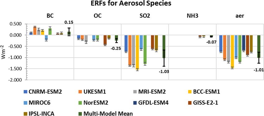
G. D. Thornhill et al.: Effective radiative forcing from emissions of reactive gases and aerosols                                    857

Table 2. List of fixed SST ERF simulations. (“NTCF” as used here excludes methane (Collins et al., 2017). Note that the abbreviation SLCFs
(short-lived climate forcers) is used in other publications to refer to near-term climate forcers.)

                                                          Aerosol                    Ozone                     Number of
               Experiment ID      CH4     N2 O          precursors               precursors     CFC / HCFC       models
               piClim-control    1850     1850               1850                      1850            1850            11
               piClim-NTCF       1850     1850               2014                      2014            1850             8
               piClim-aer        1850     1850               2014                      1850            1850             9
               piClim-BC         1850     1850     1850 (non BC)                       1850            1850             7
                                                      2014 (BC)
               piClim-O3         1850     1850               1850                      2014            1850             4
               piClim-CH4        2014     1850               1850                      1850            1850             8
               piClim-N2 O       1850     2014               1850                      1850            1850             5
               piClim-HC         1850     1850               1850                      1850            2014             6
               piClim-NOx        1850     1850               1850          1850 (non NOx )             1850             5
                                                                               2014 (NOx )
               piClim-VOC        1850     1850               1850    1850 (non CO / VOC)               1850             5
                                                                         2014 (CO / VOC)
               piClim-SO2        1850     1850    1850 (non SO2 )                      1850            1850             6
                                                      2014 (SO2 )
               piClim-OC         1850     1850     1850 (non OC)                       1850            1850             6
                                                      2014 (OC)
               piClim-NH3        1850     1850    1850 (non NH3 )                      1850            1850             2
                                                     2014 (NH3 )

to the emission or concentrations between the control and              and Soden, 2015) to break down the ERF into the instan-
perturbed runs of the models. The assumption is that there             taneous radiative forcing (IRF) and individual rapid adjust-
is minimal contribution from the climate feedback when the             ments (designated by A), which are radiative responses to
SSTs are fixed, but the resultant ERF includes rapid adjust-           changes in atmospheric state variables that are not coupled
ments to the forcing agent in the atmosphere (Forster et al.,          to surface warming. In this approach, ERF is defined as
2016).
   The ERF calculated using this method includes any con-              ERF = IRF + At_trop + At_strat + Ats + Aq + Aa + Ac + e, (1)
tributions to the ERF resulting from changes in the land
                                                                       where At_trop is the troposphere temperature adjustment,
surface temperature (Ts ), which ideally should be removed
                                                                       At_strat is the stratosphere temperature adjustment, Ats is the
(Shine et al., 2003; Hansen et al., 2005; Vial et al., 2013) (as
                                                                       surface temperature adjustment, Aq is the water vapour ad-
the ocean temperature changes are removed by using fixed
                                                                       justment, Aa is the albedo adjustment, Ac is the cloud ad-
SSTs). However, there is no simple way to prescribe land sur-
                                                                       justment, and e is the radiative kernel error. Individual rapid
face temperatures in the models considered here analogous
                                                                       adjustments (Ax ) are computed as
to fixing the SSTs, so we make the land surface temperature
correction by calculating the surface temperature adjustment                  δR
from the radiative kernel (see Sect. 3.2) and subtracting it           Ax =      dx,                                                  (2)
                                                                              δx
from the standard ERF as calculated above (see also Smith et
al., 2020a; Tang et al., 2019). This is designated the ERF_ts          where δR
                                                                              δx is the radiative kernel, a diagnostic tool typically
to differentiate it from the standard ERF as described above.          computed with an offline version of a general circulation
                                                                       model (GCM) radiative transfer model that is initialized with
3.2   Kernel analysis                                                  climatological base state data, and dx is the climate response
                                                                       of atmospheric state variable x, diagnosed directly from each
Where the relevant data are available, we use the radiative            model. Cloud rapid adjustments (AC ) are estimated by diag-
kernel method (Smith et al., 2018; Soden et al., 2008; Chung           nosing cloud radiative forcing from model flux diagnostics

https://doi.org/10.5194/acp-21-853-2021                                                       Atmos. Chem. Phys., 21, 853–874, 2021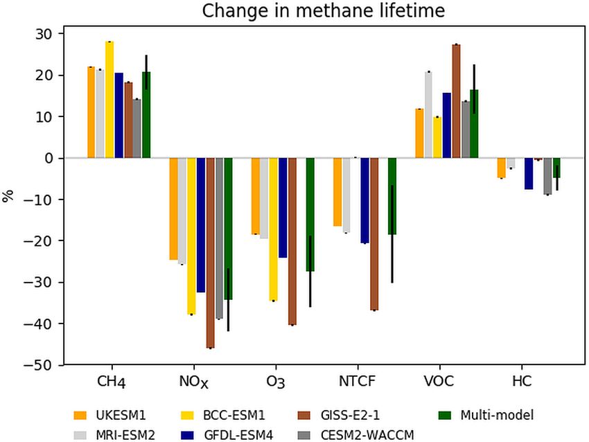
858                        G. D. Thornhill et al.: Effective radiative forcing from emissions of reactive gases and aerosols

and correcting for cloud masking using the kernel-derived         lates the cloud effects (see Eqs. 4–6, where Eq. 6 is included
non-cloud adjustments and IRF, following common practice          for completeness). The ERFaci may include non-cloud rapid
(e.g. Soden et al., 2008; Smith et al., 2018), whereby            adjustments in cloudy regions of the atmosphere. The final
                                                                  term is the ERF as calculated from fluxes with neither clouds
AC = (ERF − ERFclr ) − (IRF − IRFclr )                            nor aerosols (ERFcs, af).
                                                                     The ERFs are calculated in the same way as for the all-
       X
                               clr
     −   x=[T,ts,q,a]
                       A x − A x .                         (3)
                                                                  sky ERF described in Sect. 3.1, except that the all-sky radia-
   For the calculation of the IRF (for aerosols this is the di-   tive flux diagnostics are replaced by the relevant aerosol-free
rect effect) here, the clear-sky IRF (IRFclr ) is estimated as    fluxes for both the clear-sky and all-sky cases.
the difference between clear-sky ERF (ERFclr ) and the sum        IRFari = (ERF − ERFaf)                                       (4)
of kernel-derived clear-sky rapid adjustments (Aclr  x ). Since
estimates of Ac are dependent on IRF, the same differencing       ERFaci = ERFaf − ERFcs, af                                   (5)
method cannot be used to estimate IRF under all-sky condi-        ERFcs, af = ERFcs, af                                        (6)
tions without special diagnostics (in particular the Interna-
tional Satellite Cloud Climatology Project diagnostics (IS-         Separating the IRF in Eq. (1) into aerosols and greenhouse
CCP) diagnostics) not widely available in the AerChemMIP          gas contributions, IRF = IRFaer + IRFGHG , we can re-write
archive. Instead, for the calculations presented here all-sky     Eqs. (4)–(6).
IRF is computed by scaling IRFclr by a species-specific fac-      IRFari = IRFaer                                              (7)
tor to account for cloud masking (Soden et al., 2008).                              X
                                                                                                         clr
   Kernels are available from several sources, and for this       ERFaci =AC +     x=[T,ts,q,a]
                                                                                                 A x − A x
analysis we used kernels from CESM (Pendergrass et al.,
2018), GFDL (Soden et al., 2008), HadGEM3 (Smith et                         + IRFGHG − IRFclr GHG                              (8)
al., 2020b), and ECHAM6 (Block and Mauritsen, 2013) and                       X
                                                                  ERFcs, af =               Aclr + IRFclr
                                                                                x=[T,ts,q,a] x         GHG                     (9)
took the mean from the four kernels for each model. Overall
the individual kernels produced very similar results for each
                                                                     So ERFaci is equivalent to AC in Eq. (3) with ex-
model, as reported in Smith et al. (2018).
                                                                  tra terms to account for the all-sky–clear-sky difference
3.3   Calculation of ERF using aerosol-free radiative             in the non-cloud adjustments and all-sky–clear-sky differ-
      fluxes                                                      ence in any greenhouse gas IRF. With no greenhouse gas
                                                                  changes ERFcs,af is the total clear-sky non-cloud adjust-
To understand the contributions of various processes to the       ment. Ghan (2013) attributes this mostly to the surface
overall ERF we can attempt to separate the ERF that is due        albedo change Aclr
                                                                                  α ; however, the kernel analysis shows other
to direct radiative forcing from that due to the effects of       non-cloud adjustments are larger (Table S4). For greenhouse
clouds. Greenhouse gases and aerosols can alter the ther-         gases ERFcs,af is the total clear-sky ERF. Assuming the non-
mal structure of the atmosphere and hence cloud thermo-           cloud adjustments are small apart from Tstrat (Table S4), ER-
dynamics (the semi-direct effect (Ackerman et al., 2000),         Fcs,af is approximately SARFclr                   clr
                                                                                                    GHG . The SARFGHG is ex-
and aerosols can act via microphysical effects (e.g. increas-     pected to be an overestimate of SARFGHG by 10 %–40 %
ing the number of condensation nuclei and decreasing the          due to cloud masking (Myhre and Stordal, 1997). Thus for
effective radii of cloud droplets, referred to as the aerosol     greenhouse gases the ERFaci will be a combination of the
cloud albedo effect and the cloud lifetime effect (Twomey,        cloud adjustment and cloud masking.
1974; Albrecht, 1989; Pincus and Baker, 1994). Following
the method of Ghan (2013) the contribution of the aerosol–
                                                                  4     Results
radiation interactions to the ERF can be distinguished from
that of the aerosol–cloud interactions by using a “double-        4.1     Aerosols and precursors
call” method. This means that the model radiative flux di-
agnostics are calculated a second time but ignoring the scat-     4.1.1    Inter-model variability
tering and absorption by the aerosol – referred to in the equa-
tions below with “af”. The other effects of the aerosol on the    The ERFs are calculated as described in Sect. 3.1, and the
atmosphere (i.e. cloud changes, stability changes, dynamics       summary chart of the ERFs is shown in Fig. 1 for those mod-
changes) will still be present, however. The IRFari as defined    els with available results – it should be noted that not all mod-
here is the direct radiative forcing from the aerosol, due to     els ran all the experiments. The multi-model mean is shown
scattering and absorption of radiation. The cloud radiative       as a separate bar in Fig. 1, with the value given and the stan-
forcing (ERFaci) due to the aerosol–cloud interactions is then    dard error indicated with error bars. A table of the individual
obtained by using the difference between the aerosol-free all-    values for each model and the multi-model mean are included
sky fluxes and the aerosol-free clear-sky fluxes, which iso-      Table S2 in the Supplement.

Atmos. Chem. Phys., 21, 853–874, 2021                                                https://doi.org/10.5194/acp-21-853-2021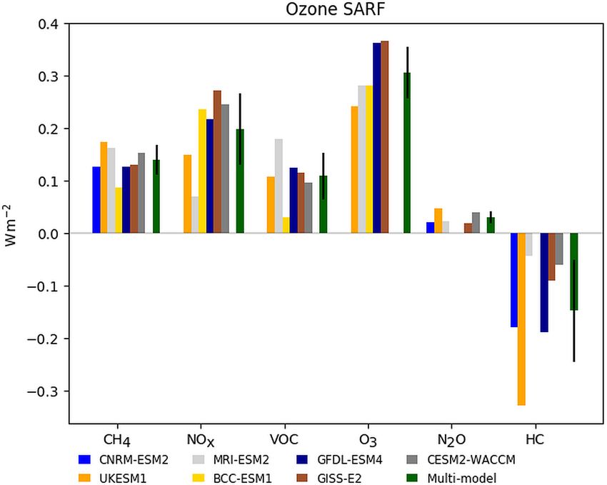
G. D. Thornhill et al.: Effective radiative forcing from emissions of reactive gases and aerosols 859
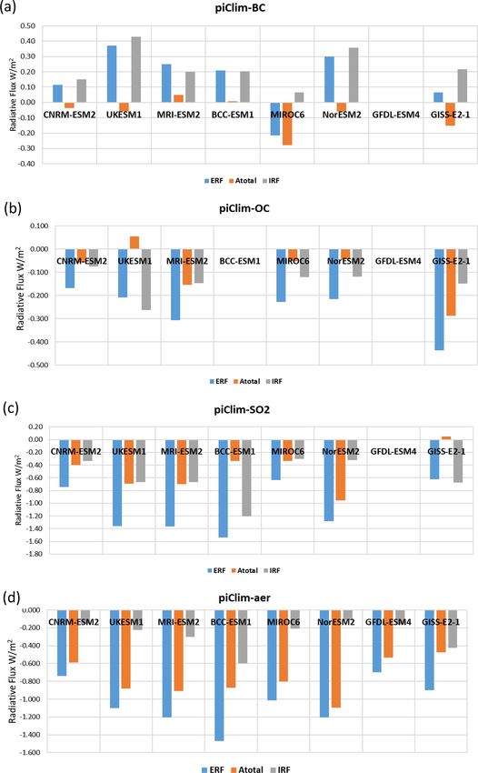
Figure 1. Aerosol ERFs for the models with the available diagnostics for the aerosol species experiments, with interannual variability
represented by error bars showing the standard error. The piClim-aer experiments include the BC and OC SO2 aerosols, and for GISS-E2-1
and IPSL-INCA NH3 aerosols are also included. The multi-model mean is shown with the mean value and error bars indicating the standard
deviation.
For the piClim-BC results, the range of values is from The issue of the effect of perturbing the pre-industrial at-
−0.21 to 0.37 W m−2 , while the MIROC6 model has a mosphere with the aerosol changes is examined in more de-
negative ERF for BC, contrasting with the positive values tail in the Supplement (see Sect. S6) for NorESM2, where a
from the other models – see further discussion on this in sensitivity analysis was carried out. This analysis does not re-
Sect. 4.1.2. peat the AerChemMIP experiments with the perturbation in
The experiments for the OC (organic carbon) have a range a present-day atmosphere but examines the effect of adding
from −0.44 to −0.15 W m−2 , and the variability between the the SO2 and combined aerosol perturbation to an already
models is much less than for the other experiments. The cal- polluted present-day atmosphere. In this simplified sensitiv-
culated ERFs for the SO2 experiment show a variation from ity study the differences are 13 % for the SO2 experiment
−1.54 to −0.62 W m−2 , with CNRM-ESM2-1, MIROC6, and 20 % for the combined aerosol experiment. However, it
IPSL-INCA and GISS-E2-1 at the lower end of the range. should be borne in mind that this is for a specific model, and
These models show a smaller rapid adjustment to clouds the perturbed experiment still has the 1850 climate condi-
which would account for this (see Fig. S1); also note that tions.
CNRM-ESM2-1 does not include aerosol effects apart from The ERF_ts is a simplified method for corrections of land
the cloud albedo effect. The two models with results for the surface warming in fixed sea surface temperature simulations
NH3 (GISS-E2-1 and IPSL-INCA) experiment have ERFs of which in addition to land surface changes leads to changes in
−0.08 and −0.06 W m−2 respectively. land surface albedo changes, tropospheric temperature, water
The piClim-aer experiment which uses the 2014 values of vapour and cloud changes (Smith et al., 2020a; Tang et al.,
aerosol precursors and PI (pre-industrial) values for CH4 , 2019).
N2 O and ozone precursors shows a range from −1.47 to The ERF_ts values for the models where the land surface
−0.7 W m−2 among the models, making it difficult to nar- temperature adjustment is removed are also included in Sup-
row the range of uncertainty of aerosols from global mod- plement Tables S2 and S3 for comparison with the standard
els. However, the range in the CMIP6 models is consistent ERF. In general, the difference between the two values is
with that reported in Bellouin et al. (2019), who suggest small, of the order of 5 %–10 %.
a probable range of −1.60 to −0.65 W m−2 for the total
aerosol ERF, and compares well with the range of −1.37 to 4.1.2 Breakdown of the ERF into atmospheric
−0.63 W m−2 for the set of piClim-aer experiments consid- adjustments and IRF
ered in Smith et al. (2020a) as part of the RFMIP project. In
general, the sum of the ERFs from the individual BC, OC and The results in Fig. 2 show the ERF as calculated from the
SO2 experiments does not equal the piClim-aer experiment, radiative fluxes in the fixed SST experiments (Sect. 3.1),
due to non-linearity in the aerosol–cloud interactions, par- the total of the atmospheric adjustments, Atotal , described in
ticularly since the aerosol perturbation is added to the rela- Sect. 3.2 (where Atotal = AT + Ats + Aq + Aa + Ac cf. Eq. 1),
tively pristine pre-industrial atmosphere. In the case of GISS, and the instantaneous radiative forcing (IRF).
IPSL-INCA and GFDL-ESM4 the models also include ni- The sum of the IRF and the atmospheric adjustments
trate aerosols. should equal the overall ERF; however, as the calculation of
the IRF depends upon an empirical factor for cloud masking
https://doi.org/10.5194/acp-21-853-2021 Atmos. Chem. Phys., 21, 853–874, 2021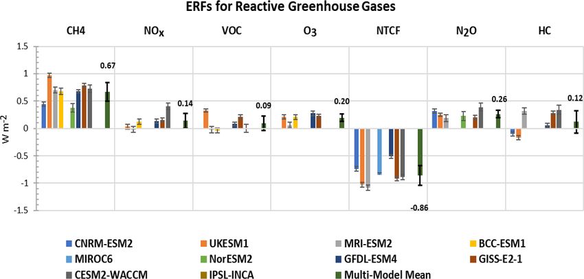
860                         G. D. Thornhill et al.: Effective radiative forcing from emissions of reactive gases and aerosols

Figure 2. Breakdown of the ERFs into the atmospheric rapid adjustments (Atotal) and IRF (instantaneous radiative forcing) for the aerosols.
(a) piClim-BC experiment; (b) piClim-SO2 experiment; (c) piClim-OC experiment; (d) piClim-aer experiment.

Atmos. Chem. Phys., 21, 853–874, 2021                                                       https://doi.org/10.5194/acp-21-853-2021
G. D. Thornhill et al.: Effective radiative forcing from emissions of reactive gases and aerosols                              861

                                                                   the increase in low clouds reported for this model, and the
                                                                   treatment of BC as ice nuclei causes the large negative cloud
                                                                   adjustment here (Takemura and Suzuki, 2019; Suzuki and
                                                                   Takemura, 2019). The GISS-E2-1 model also has a strong
                                                                   cloud rapid adjustment, but the larger positive value of the
                                                                   IRF leads to an overall positive ERF for this model. With the
                                                                   exception of MIROC6 the negative tropospheric temperature
                                                                   adjustment is balanced by the water vapour (specific humid-
                                                                   ity) adjustment, although the magnitude of these adjustments
                                                                   for MRI-ESM2 is at least twice that for the other two models.
                                                                   The interaction of BC with clouds in the MRI-ESM2 model
                                                                   is discussed in detail in Oshima et al. (2020), in particular the
                                                                   impact of BC on ice nucleation in high clouds. The larger sur-
Figure 3. Breakdown of the atmospheric adjustments (albedo,        face albedo adjustment for both NorESM2 and MRI-ESM2
cloud, water vapour, troposphere temperature, stratosphere tem-
                                                                   is most likely due to the representation of deposition of BC
perature and surface temperature) for the piClim-BC experiments,
                                                                   on snow and ice in these models (Oshima et al., 2020).
showing the variability between models.
                                                                      The piClim-aer experiments (Fig. 1d) show all models
                                                                   have a negative Atotal , covering a range from −0.47 to
                                                                   −1.1 W m−2 . Overall, the cloud rapid adjustments dominate
to find the all-sky IRF from the clear-sky IRF (see Sect. 3.2)     for the piClim-aer experiments, with a contribution rang-
the sum of the IRF and the Atotal will not necessarily equal       ing from −0.45 to −1.1 W m−2 (See Fig. S1). Smith et
the ERF as calculated directly from the model radiative flux       al. (2020a) also recently diagnosed forcing and adjustments
diagnostics. However, in general the difference is less than       in a similar subset of CMIP6 models for the piClim-aer ex-
3 %, suggesting that the approximation used in the calcula-        periment as part of the Radiative Forcing Model Intercom-
tion of the IRF is reasonable. Using the kernel method de-         parison Project (RFMIP) efforts. While they also diagnosed
scribed above it is important to note that the IRF calculated      IRF as a residual calculation between ERF and the sum of
here accounts for the presence of the clouds but does not in-      rapid adjustments, they estimated cloud adjustments using a
clude cloud changes such as the cloud albedo effect.               modified version of the approximate partial radiative pertur-
   The models show a variability in the IRF for SO2 (Fig. 2c),     bation (APRP) method instead of radiative kernels. In their
with a range of −0.3 to −1.2 W m−2 with the BCC-                   approach, the cloud albedo effect (i.e. Twomey effect) is con-
ESM1 model being the outlier, having the largest overall           sidered part of the IRF, whereas in the traditional kernel de-
ERF. The OC experiments (Fig. 2b) range from −0.08 to              composition, it is considered a cloud adjustment. Table S5
−0.26 W m−2 , with a range for BC of 0.07 to 0.43 W m−2            compares the two sets of estimates, highlighting the IRF and
(Fig. 2a). In MIROC6 the treatment of BC (Takemura and             total cloud adjustment exhibit a near-equal absolute differ-
Suzuki, 2019; Suzuki and Takemura, 2019) leads to faster           ence between the two studies, and the sum of IRF and total
wet removal of BC and hence a lower IRF. For the combined          cloud adjustment is in close agreement (mean % difference
aerosols (Fig. 2d) the range is from −0.1 to −0.6 W m−2 .          ∼ 1.0 % for this subset of models). This indicates the classi-
   There are significant differences between the models in         fication of the first indirect effect is the only noticeable dif-
the Atotal for SO2 ; these range from 0.05 to −1.0 W m−2 ,         ference between the two approaches.
where the differences are dominated by the cloud adjust-              The breakdown of the rapid adjustments for all the models
ments which here include the cloud albedo effect as part           is included in Fig. S1, showing the contributions from each
of the adjustment (see Fig. S3 for breakdowns of the atmo-         type of rapid adjustment for all the experiments for which we
spheric adjustments for all models). The adjustments to BC         have the relevant diagnostics.
vary in sign and magnitude, with the MRI-ESM2 and BCC-
ESM1 models having a slight positive adjustment. The over-         4.1.3   Radiation and cloud interactions
all model mean has a weaker negative adjustment to that re-
ported by Stjern et al. (2017), Samset et al. (2016) and Smith     The second method of breaking down the ERF to constituents
et al. (2018). The MIROC6 model has a large negative ad-           is described in Sect. 3.3 (the Ghan method), the results from
justment which is large enough to lead to an overall negative      which are shown in Table 3. The detailed ERF results for
ERF. We explore the contribution of the individual adjust-         MRI-ESM2 are summarized in Oshima et al. (2020) and for
ments to BC in more detail in Fig. 3.                              UKESM1 in O’Connor et al. (2020a). Only four of the mod-
   Examining the breakdown of the rapid adjustments for the        els under consideration have so far produced the necessary
piClim-BC experiments (Fig. 3) we see considerable vari-           diagnostics for this calculation, and the results are presented
ability in the relative importance of the rapid adjustments;       in Table 3. For the experiments on aerosols (aer, BC, SO2 ,
the cloud adjustment dominates in MIROC6, consistent with          OC) the ERFcs,af (non-cloud adjustments) contribution is

https://doi.org/10.5194/acp-21-853-2021                                                Atmos. Chem. Phys., 21, 853–874, 2021
862 G. D. Thornhill et al.: Effective radiative forcing from emissions of reactive gases and aerosols
Table 3. Results for IRFari, ERFaci and ERFcs,af for aerosol experiments from several models.
UKESM1 CNRM-ESM2 NorESM2 MRI-ESM2
IRFari ERFcs,af ERFaci IRFari ERFcs,af ERFaci IRFari ERFcs,af ERFaci IRFari ERFcs,af ERFaci
aer −0.15 0.05 −1.00 −0.21 0.08 −0.61 0.03 −0.03 −1.21 −0.32 0.09 −0.98
BC 0.37 0.001 −0.005 0.13 0.01 −0.03 0.35 0.07 −0.12 0.26 0.08 −0.09
OC −0.15 −0.01 −0.07 −0.07 0.04 −0.14 −0.07 0.02 −0.16 −0.07 −0.05 −0.21
SO2 −0.49 0.03 −0.91 −0.29 0.08 −0.53 −0.19 −0.09 −1.01 −0.48 0.05 −0.93
small, and the ERF is largely a combination of the direct ra- Table 4. Values of ERF, 1AOD and ERF / AOD for aerosol exper-
diative effect, IRFari, and the cloud radiative effect, ERFaci. iments for CNRM-ESM2-, MIROC6, Nor-ESM2, GISS-E2-1 and
The IRFari is the direct effect of the aerosol due to scattering MRI-ESM2 models.
and absorption, while the ERFaci is the contribution from the
aerosol–cloud interactions and is approximately equal to the Change in
BC exp. BC ERF BC AOD ERF / AOD
rapid adjustments due to clouds (Ac see Sect. 3.2).
For the BC experiment the contribution of the aerosol– CNRM-ESM2 0.114 0.0015 77.64
cloud interaction has a strong contribution to the overall ERF, MIROC6 −0.214 0.0006 −339.38
except in the case of UKESM1 where it is much weaker; NorESM2 0.300 0.0019 159.75
this may be due to the strong short-wave (SW) and long- GISS-E2-1 0.065 0.002 31.65
wave (LW) cloud adjustments in this model cancelling out MRI-ESM2 0.251 0.0073 34.22
(O’Connor et al., 2020a; Johnson et al., 2019). The SO2 ex- Change in
periment shows a large cloud radiative effect; in fact the ER- OC exp. OC ERF OA AOD ERF / AOD
Faci is mostly double the IRFari in all the models, due to the
CNRM-ESM2 −0.169 0.0030 −57.20
large effect on clouds of SO2 and sulfates through the indi- MIROC6 −0.227 0.0065 −35.05
rect effects. For the OC experiments the ERFaci to IRFari NorESM2 −0.215 0.0053 −40.57
comparison is mixed, with the ERFaci general half or less GISS-E2-1 −0.438 0.0041 −107.16
the IRFari, except in the case of UKESM1, where this ratio MRI-ESM2 −0.317 0.0034 −94.39
is reversed.
Change in
The IRFari values are compared with the IRF calculated
SO2 exp. SO2 ERF SO4 AOD ERF / AOD
via the kernel analysis (Sect. 3.2) where the relevant model
results are available. These are shown in Fig. S2a; the agree- CNRM-ESM2 −0.746 0.0118 −63.22
ment is generally good, giving confidence in the kernel anal- MIROC6 −0.637 0.0152 −41.91
ysis. Similarly, ERFaci compares well with the cloud adjust- NorESM2 −1.281 0.0099 −129.24
GISS-E2-1 −0.622 0.0308 −20.22
ment Ac (Fig. S2b).
MRI-ESM2 −1.365 0.0279 −49.08
4.1.4 AOD forcing efficiencies
In order to break down the contributions of the constituent piClim-OC experiments for each of the five models which
aerosol species to the overall aerosol ERF, we use the AOD had the relevant optical depth diagnostics available.
(aerosol optical depth) as a forcing efficiency metric for each The MIROC6 model results in a negative scaling for BC
of the species and use this to assess their contributions to the due to the negative ERF for this experiment for this model
overall ERF. Not all models had diagnostics available for the (Takemura and Suzuki, 2019; Suzuki and Takemura, 2019)
AOD for the individual species, so the analysis uses a subset (see Sect. 4.1.1). The change in the BC AOD is similar for
of the models. CNRM-ESM2-1 and Nor-ESM2, and the scale factors reflect
By looking at the single species piClim-BC, piClim-OC the differences in the ERF. The scaling for the SO4 in the
and piClim-SO2 experiments, we can find the change in the NorESM2 experiment is twice that of the other models, sug-
AOD for the individual species (e.g. 1AOD for BC for the gesting a larger impact of the SO4 AOD on the ERF in this
piClim-BC experiment) and use this to scale the piClim-BC model. These values differ somewhat from those found in
ERF using the AOD change. This assumes that the ERF in Myhre et al. (2013b), where they examined the radiative forc-
the single-species experiment is wholly due to the change in ing normalized to the AOD using models in the AeroCom
that species as indicated by the AOD, an assumption which phase II experiments. They found values for sulfate ranging
is explored in the Supplement in Sect. S4. Table 4 shows the from −8 to −21 W m−2 per unit AOD, which is much weaker
AOD forcing efficiency for the piClim-BC, piClim-SO2 and than those in our results. However, it is important to note that
Atmos. Chem. Phys., 21, 853–874, 2021 https://doi.org/10.5194/acp-21-853-2021G. D. Thornhill et al.: Effective radiative forcing from emissions of reactive gases and aerosols 863 Figure 4. The contributions to the ERF for piClim-aer from the individual species, the sum of the scaled ERFs and the ERF calculated directly from the piClim-aer experiment for five of the models. in the AeroCom phase II experiments the cloud and cloud experiment (NB the sea salt and dust contributions to the optical properties are identical between their control and per- ERF are less than 1 %, and they are not shown in this fig- turbed runs, so no aerosol indirect effects are included, nor ure for clarity – the ERF / AOD forcing efficiency for these are any rapid adjustments (IRFari in Eq. 4). For the BC ex- is presented in Thornhill et al. (2020). There is considerable periment their values range from 84 to 216 W m−2 per unit variation in the ERF for the piClim-aer experiments between AOD, broadly similar to the results presented here (with the models (see Sect. 4.1), but from this analysis the SO4 is the exception of the negative MIROC6 result). Their results for largest contributor in all cases, although in the case of the OA (organic aerosols) which include fossil fuel and biofuel MIROC6 model its relative importance is reduced. The pos- emissions have values ranging from −10 to −26 W m−2 per itive ERF contribution from the BC tends to partly offset the unit AOD – weaker than our values for the piClim-OC ex- negative ERF from the OA and SO4 , except in the MIROC6 periments, which range from −35 to −107 W m−2 per unit model, where the BC has a negative contribution to the ERF. AOD but include the cloud indirect effects here. The difference between the calculated ERF from the sum The sum of the individual AODs from BC, SO4 , OA, dust of the scaled ERFs is a result of the non-linearity of the and sea salt gives the total aerosol AOD in the piClim-aer aerosol–cloud interactions, a factor which is increased be- experiment, where the various aerosols were combined. We cause the aerosols are added to the pre-industrial atmosphere. can then use the AOD for each aerosol in the piClim-aer ex- However, using the IRFari instead of the total ERF to calcu- periment and the forcing efficiency above to find the contri- late the forcing efficiency and using the same method also bution of the individual aerosol to the overall change in ERF, results in a difference between the total IRFari derived from providing an approximate estimate of the relative contribu- the scaled individual experiments and the IRFari for the com- tion of each aerosol to the overall ERF. In Fig. 4 the relative bined aerosol experiment, suggesting that the difference is contributions to the ERF from black carbon (BC), organic not simply a result of the aerosol–cloud interactions. aerosols (OA) and sulfate (SO4 ) are shown for three of the Using the burden as a scaling factor following the same models. The sum of the ERFs from the individual species analysis as described for the AOD results in a largely similar is also compared to the ERF calculated from the piClim-aer result for the scaling factor, although interestingly the bur- https://doi.org/10.5194/acp-21-853-2021 Atmos. Chem. Phys., 21, 853–874, 2021
864 G. D. Thornhill et al.: Effective radiative forcing from emissions of reactive gases and aerosols
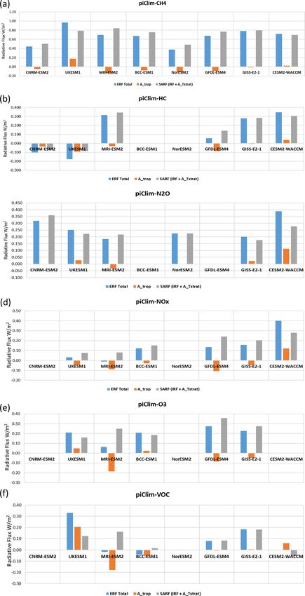
Figure 5. Reactive gas ERFs for the models with the available diagnostics for the reactive gas experiments with interannual variability
represented by error bars showing the standard error. The multi-model mean is shown with the mean value and error bars indicating the
standard deviation.
den scaling for SO2 in the Nor-ESM2 model is similar to the For gas-phase experiments the diagnosed cloud interac-
other models (see Table S6 for the burden forcing efficiency). tions (ERFaf–ERFcs,af) comprise the ERFaci from effects
on aerosol chemistry (as in Sect. 3.3) but also any cloud ad-
justments and effects of cloud masking on the gas-phase forc-
4.2 Reactive greenhouse gases
ing (Eq. 8). The clear-sky aerosol-free diagnostic (ERFcs,af)
is an indication of the greenhouse gas forcing; however, this
The different Earth system models include different de- will be an overestimate as it neglects cloud masking effects
grees of complexity in their chemistry, so their responses (Sect. 3.3).
to changes in reactive gas concentrations or emissions dif-
fer. NorESM2 has no atmospheric chemistry, so there is no
change to ozone (tropospheric or stratosphere) or to aerosol 4.2.1 ERF vs. SARF
oxidation following changes in methane or N2 O concentra-
tions. CNRM-ESM2-1 includes stratospheric ozone chem- For the reactive greenhouse gases the kernel analysis is used
istry but no non-methane hydrocarbon chemistry, and thus to break down the ERF into the stratospherically adjusted ra-
ozone is prescribed below 560 hPa. There are no effects of diative forcing (SARF), which is calculated using the IRF
chemistry on aerosol oxidation. BCC-ESM1 includes tro- from the kernel analysis (Sect. 3.2), the stratospheric temper-
pospheric chemistry but not stratospheric chemistry. Strato- ature adjustment (At_strat ) (SARF = IRF + At_strat ), and the
spheric concentrations are relaxed towards climatological tropospheric adjustments (Atrop ), which is the sum of the
values. UKESM1, GFDL-ESM4, CESM2-WACCM, GISS- tropospheric atmospheric adjustments. These quantities are
E2 and MRI-ESM2 all include tropospheric and stratospheric plotted in Fig. 6.
ozone chemistry as well as changes to aerosol oxidation For methane the ERFs are largest for those models that in-
rates. The ERFs calculated for the reactive gases for sev- clude tropospheric ozone chemistry reflecting the increased
eral models are shown in Fig. 5, with the multi-model means forcing from ozone production (see Sect. 4.2.2). The ana-
given in Table S3. lytic calculation for CH4 only based on Etminan et al. (2016)
The contributions from gas-phase and aerosol changes to gives a SARF of 0.56 W m−2 . The tropospheric adjustments
the ERF can be pulled apart to some extent by using the are negative for all models except UKESM1 (Fig. 6). The
clear-sky and aerosol-free radiation diagnostics (Table 5). negative cloud adjustment comes from an increase in the
The direct aerosol forcing (IRFari) is diagnosed as for the LW emissions, possibly due to less high cloud. In UKESM1
aerosol experiments (Sect. 3.3). The diagnosed changes in O’Connor et al. (2020b) show that methane decreases sul-
aerosol mass are shown in Table S8. GFDL-ESM4 and GISS- fate new particle formation, thus reducing cloud albedo and
ES-1 include nitrate aerosol and show expected responses hence a positive cloud adjustment in that model.
from NOX emissions (including O3 experiment). CESM2- For N2 O, results are available for models CNRM-ESM2,
WACCM shows an increase in secondary organic aerosol NorESM2, MRI-ESM2 and GISS-E2 (the analytic N2 O-only
from VOC emissions. Sulfate responses are generally incon- calculation gives a SARF of 0.17 W m−2 ). There appears to
sistent across the models. There seems little correlation be- be little net rapid adjustment to N2 O apart from CESM2-
tween aerosol mass changes and diagnosed IRFari. WACCM. Note that due to the method of calculating the all-
Atmos. Chem. Phys., 21, 853–874, 2021 https://doi.org/10.5194/acp-21-853-2021G. D. Thornhill et al.: Effective radiative forcing from emissions of reactive gases and aerosols 865
Table 5. Calculations of IRFari, ERFaci (cloud) and ERFcs,af for the chemically reactive species.
UKESM GFDL-ESM4 CNRM-ESM2 NorESM2 MRI-ESM2
IRFari ERFcs,af cloud IRFari ERFcs,af cloud IRFari ERFcs,af cloud IRFari ERFcs,af cloud IRFari ERFcs,af cloud
CH4 −0.01 0.86 0.12 −0.01 0.91 −0.22 0.00 0.56 −0.12 −0.01 0.48 −0.10 0.00 0.91 −0.21
HC −0.02 0.02 −0.18 −0.02 0.22 −0.14 −0.01 −0.02 −0.08 −0.02 0.50 −0.17
N2 O −0.01 0.26 0.01 0.00 0.41 −0.09 −0.01 0.24 −0.00 −0.00 0.23 −0.03
O3 −0.02 0.16 0.07 −0.04 0.49 −0.18 −0.00 0.24 −0.18
NOx −0.03 0.10 −0.05 −0.02 0.25 −0.09 −0.01 0.03 −0.04
VOC 0.00 0.13 0.20 −0.02 0.18 −0.08 0.004 0.17 −0.2
sky IRF (Sect. 3.2), the IRF and the adjustment terms do not 4.2.3 Comparison with greenhouse gas forcings
sum to give the ERF.
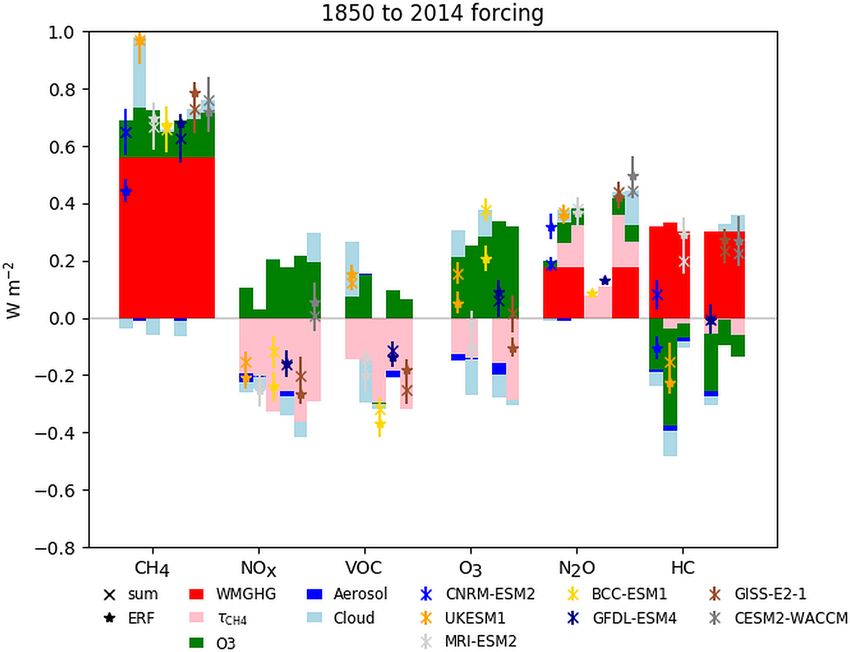
The models respond very differently to changes in halocar- The ERFs, ERFcs,af and SARFs diagnosed for the green-
bons. The expected halocarbon-only SARF is +0.30 W m−2 house gas changes (Fig. 6, Table 5) are compared with the
depending on exact speciation used in the model (WMO, expected greenhouse gas SARFs in Fig. 8. The expected
2018). For CNRM-ESM2, UKESM1 and GFDL-ESM4, the SARFs from the well-mixed gases are given by Etminan et
ERFs are negative or only slightly positive (see also Mor- al. (2016) for CH4 and N2 O and by WMO (2018) for the
genstern et al., 2020), whereas for GISSE21 and MRI-ESM2 halocarbons (the halocarbon changes are slightly different in
the ERFs and SARF are both strongly positive. The differ- each model). The expected SARFs from ozone changes are
ences in stratospheric ozone destruction in these models can from Fig. 7.
partially explain the inter-model differences (Sect. 4.2.2). For methane the ERFs are typically higher than the ex-
pected GHG SARF (except for CNRM-ESM2). The diag-
nosed ERFcs,af and SARF agree better with the expected
4.2.2 Ozone changes SARF in UKESM1, BCC-ESM1 and CESM2-WACCM but
not in other models. For N2 O the modelled ERF is larger
The ozone radiative forcing is diagnosed using a kernel to than the expected SARF for CNRM-ESM2-1 and CESM2-
scale the 3D ozone changes based on Skeie et al. (2020). This WACCM; this is explained by the rapid adjustments for
kernel includes stratospheric temperature adjustment, but not CESM2-WACCM but not for CNRM-ESM2. For halocar-
tropospheric adjustments and thus gives a SARF. These are bons the stratospheric ozone depletion offsets the direct
shown in Fig. 7. Corresponding changes in the tropospheric SARF and accounts for much of the spread in the model
and stratospheric ozone columns are shown in Fig. S5, In- SARF, although the CNRM-ESM2-1 ERF and SARF are
creased CH4 concentrations give a SARF for ozone pro- lower than expected. The modelled HC ERF for UKESM1
duced by methane of 0.14 ± 0.03 W m−2 , and anthropogenic is strongly negative due to increased aerosol–cloud interac-
NOx emissions and VOC (including CO) emissions give tions (O’Connor et al., 2020a; Morgenstern et al., 2020), but
SARFs of 0.20 ± 0.07 and 0.11 ± 0.04 W m−2 respectively. removing cloud effects using the SARF or ERFcs,af agrees
The O3 experiment comprised both NOx and VOC emission better with the expected value. The estimated ozone SARF
changes. The SARF in this experiment (0.31 ± 0.05 W m−2 ) from the NOX , VOC and O3 experiments generally agrees
is close to the sum of the NOx and VOC experiments with the model SARF and ERFcs,af. For CESM2-WACCM
(0.30 ± 0.05 W m−2 for the same set of models) showing lit- the ERF from the VOC experiment is zero, and the SARF is
tle non-linearity in the chemistry (Stevenson et al., 2013). negative even though the diagnosed ozone SARF is positive.
There is a larger variation across models in the For all experiments and models ERFcs,af is generally higher
stratospheric ozone depletion from halocarbons (−0.15 ± than the expected or diagnosed SARF (see Sect. 3.3).
0.10 W m−2 ), with UKESM1 having noticeably larger de-
pletion as seen in Keeble et al. (2020), giving a SARF of 4.2.4 Methane lifetime
−0.33 W m−2 . N2 O causes some stratospheric ozone deple-
tion in these models, mainly in the tropical upper stratosphere In the CMIP6 set-up the modelled methane concentrations do
where depletion causes a positive forcing (Skeie et al., 2020), not respond to changes in oxidation rates. The methane life-
and increases tropospheric ozone (Fig. S6), giving a small net time is diagnosed (which includes stratospheric loss to OH
positive SARF (0.03 ± 0.01 W m−2 ). as parameterized within each model), and, assuming losses
Methane oxidation also leads to water vapour production. to chlorine oxidation and soil uptake of 11 and 30 Tg yr−1
Figure S6 shows increases in the stratosphere for the piClim- (Saunois et al., 2020; Myhre et al., 2013b), this can be used to
CH4 of up to 20 % . The kernel analysis however finds very infer the methane changes that would be expected if methane
low radiative forcing associated with this increase (−0.002± were allowed to vary. Figure 9 shows the methane lifetime
0.003 W m−2 ). response is large and negative for NOx emissions, with a
https://doi.org/10.5194/acp-21-853-2021 Atmos. Chem. Phys., 21, 853–874, 2021You can also read


