An Overview of Geoengineering of Climate using Stratospheric Sulfate Aerosols
←
→
Page content transcription
If your browser does not render page correctly, please read the page content below
An Overview of Geoengineering of Climate
                        using Stratospheric Sulfate Aerosols

                 Philip J. Rasch1∗ , Simone Tilmes1 , Richard P. Turco 2 , Alan Robock3 , Luke Oman4 ,
                                   Chih-Chieh (Jack) Chen1 , Georgiy L. Stenchikov3
       1
         National Center for Atmospheric Research, P.O. Box 3000-80307, Boulder CO 80307, USA
       2
         Department of Atmospheric and Oceanic Sciences, University of California, Los Angeles, CA,
           90095-1565, USA
       3
         Department of Environmental Sciences, Rutgers University, New Brunswick, NJ 08901, USA
       4
         Department of Earth and Planetary Sciences, Johns Hopkins University, Baltimore , MD 21218, USA
       ∗
         To whom correspondence should be addressed; Phone: 303-497-1368; E-mail: pjr@ucar.edu.

                                         Printed: March 11, 2008

0
    The National Center for Atmospheric Research is sponsored by the National Science Foundation
1 Abstract 2 We provide an overview of geoengineering by stratospheric sulfate aerosols. We review the state of understanding 3 about this topic as of early 2008, summarizing the past 30 years of work in the area, and highlight some very recent 4 studies using general circulation models of the atmosphere and ocean, and discuss the efficacy of producing such 5 aerosols by methods used to deliver sulfur species to the stratosphere. 6 The studies reviewed here all suggest that sulfate aerosols can counteract the globally averaged temperature 7 increase associated with increasing greenhouse gases, and reduce changes to some other components of the earth 8 system. There are likely to be remaining regional climate changes after geoengineering, with some regions expe- 9 riencing significant changes in temperature or precipitation. The aerosols also serve as surfaces for heterogeneous 10 chemistry resulting in increased ozone depletion for several decades. We conclude by highlighting many of the 11 areas where more research is needed.
12 1 Introduction
13 The concept of “geoengineering”(the deliberate change of the Earths’ Climate by mankind (Keith, 2000)) has been
14 considered at least as far back as the 1830s with J.P. Espy’s suggestion (Fleming, 1990) of lighting huge fires that
15 would stimulate convective updrafts and change rain intensity and frequency of occurence. Geoengineering has
16 been considered for many reasons since then ranging from making polar latitudes habitable to changing precipita-
17 tion patterns. The history of geoengineering is reviewed elsewhere in this volume.
18 There is increasing concern by scientists and society in general that energy system transformation is proceed-
19 ing too slowly to avoid the risk of dangerous climate change from humankind’s release of radiatively important
20 atmospheric constituents (particularly CO2 ). The assessment by the Intergovernmental Panel on Climate Change
21 (IPCC, 2007c) shows that unambiguous indicators of human-induced climate change are increasingly evident, and
22 there has been little societal response to the scientific consensus that reductions must take place soon to avoid large
23 and undesirable impacts.
24 The first response of society to this evidence ought to be to reduce greenhouse gas emissions, but if one
25 accepts the evidence, and notes the inertia to changing our energy infrastructure, a second step might be to explore
26 strategies to mitigate some of the planetary warming. For this reason geoengineering for the purpose of cooling
27 the planet is receiving increasing attention. A broad overview to geoengineering can be found in the reviews of
28 Keith (2000), WRMSR (2007), and the papers in this volume. The geoengineering paradigm is not without its own
29 perils (Robock, 2008). Some of the uncertainties and consequences of the approach explored here are discussed in
30 this article. Others can be found elsewhere in this volume.
31 This study describes an approach to cooling the planet that goes back at least as far as 1974, when Budyko, in
32 a series of studies (e.g., Budyko, 1974)) suggested that if global warming ever became a serious threat, we could
33 counter it with airplane flights in the stratosphere, burning sulfur to make aerosols that would reflect sunlight away.
34 The aerosols would increase the planetary albedo, and cool the planet, ameliorating some (but as discussed below,
35 not all) of the effects of increasing CO2 concentrations.
36 Sulfate aerosols are always found in the stratosphere. Low background concentrations arise due to transport
37 from the troposphere of natural and anthropogenic sulfur-bearing compounds. Occasionally much higher concen-
38 trations arise from the volcanic eruptions, resulting in a temporary cooling of the Earth system (Robock, 2000),
39 which disappears as the aerosol is flushed from the atmosphere. The volcanic injection of sulfate aerosol thus
40 serves as a natural analog to the geoengineering aerosol. The analogy is not perfect, because the volcanic aerosol
41 is flushed within a few years, and the climate system does not respond the same way as it would if the particles
42 were continually replenished, as they would be in a geoengineering effort. Perturbations to the system, which
43 might become evident with constant forcing, disappear as the forcing disappears.
44 This study reviews the state of understanding about geoengineering by sulfate aerosols, as of early 2008. We
45 review the published literature, introduce some new material, and summarize some very recent results that are
46 presented in detail in submitted articles at the time of the writing of this article. In our summary we also try to
47 identify areas where more research is needed.
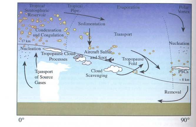
48 2 Review
49 Since the paper by Budyko (1974), the ideas generated there have received occasional attention in discussions
50 about geoengineering (e.g., NAS92, 1992; Turco, 1995; Govindasamy and Caldeira, 2000; Govindasamy et al.,
51 2002; Govindasamy and Caldeira, 2003; Crutzen, 2006; Wigley, 2006; Matthews and Caldeira, 2007).
52 There are also legal, moral, ethical, financial, and international political issues associated with a manipulation
53 of our environment. Commentaries (Lawrence, 2006; Bengtsson, 2006; Kiehl, 2006; Cicerone, 2006; MacCracken,
54 2006) to Crutzen (2006) address some of these issues and remind us that this approach does not treat all the
55 consequences of higher CO2 concentrations (such as ocean acidification; others are discussed in Robock (2008)).
156 Recently, climate modellers have begun efforts to provide more quantitative assessments of the complexities of
57 geoengineering by sulfate aerosols and the consequences to the climate system (Rasch et al., 2008; Robock et al.,
58 2008; Tilmes et al., 2008b,a).
59 3 An overview of Stratospheric aerosols in the Earth System
60 3.1 General considerations:
Figure 1: A schematic of the processes that influence the life cycle of stratospheric aerosols (from SPARC (2006),
with permission)
61 Sulfate aerosols are an important component of the Earth system in the troposphere and stratosphere. Because
62 sulfate aerosols play a critical role in the chemistry of the lower stratosphere and occasionally, following a volcanic
63 eruption, in the radiative budget of the Earth by reducing the incoming solar energy reaching the Earth surface,
64 they have been studied for many years. A comprehensive discussion of the processes that govern the stratospheric
65 sulfur cycle can be found in the recent assessment of stratosphere aerosols (SPARC, 2006). Figure 1 taken from
66 that report indicates some of the processes that are important in that region.
67 Sulfate aerosols play addional roles in the troposphere (IPCC, 2007c, and the references therein). As in the
68 stratosphere they act to reflect incoming solar energy (the “aerosol direct effect”), but also act as cloud condensation
69 nuclei, influencing the size of cloud droplets, and the persistence or lifetime of clouds (the “aerosol indirect effect”),
70 and thus the reflectivity of clouds.
71 Although our focus is on stratospheric aerosols, one cannot ignore the troposphere, and so we include a brief
72 discussion of some aspects of the tropospheric sulfur cycle also. A very rough budget describing the sources,
20.0001 0.3 0.03 0.01 0.06 0.2
(13 days) (10 years) (30 days) (2 years)
0.1
(Sed)
0.004 0.03 Tropopause 0.03 0.06
15
0.06 2 2 0.4 50 0.6
(1.4 days) (1 year) (2 days) (5 days)
15 2 65 32 1 51
Surface (Scav)
CS2,H2S,DMS OCS SO2 SO4=
Figure 2: A very rough budget (about 1 digit of accuracy) for most of the major atmospheric sulfur species during
volcanically quiescent situations, following Rasch et al. (2000),Montzka et al. (2007) and SPARC (2006). Numbers
inside boxes indicate species burden in units of Tg S, and approximate lifetime against the strongest source or
sink. Numbers beside arrows indicate net source or sinks (transformation, transport, emissions, and deposition
processes) in Tg S/yr.
73 sinks, and transformation pathways during volcanically quiescent times is displayed in figure 21 Sources, sinks,
74 and burdens for sulfur species are much larger in the troposphere than the stratosphere. The source of the aerosol
75 precursors are natural and anthropogenic sulfur bearing reduced gases (DMS, SO2 , H2 S, OCS). These precursor
76 gases are gradually oxidized (through both gaseous and aqueous reactions) to end products involving the sulfate
77 anion (SO2−4 ) in combination with various other cations. In the troposphere where there is sufficient ammonia,
78 much of the aerosol exists in the form of mixtures of ammonium sulfate ((NH4 )2 SO4 ) and bisulfate ((NH4 )HSO4 ).
79 The stratospheric sulfur bearing gases oxidize (primarily via reactions with the OH radical) to SO2 , which is
80 then further oxidized to gaseous H2 SO4 . Stratospheric sulfate aerosols exist in the form of mixtures of condensed
81 sulfuric acid (H2 SO4 ), water, and under some circumstances, hydrates with nitric acid (HNO3 ).
82 Although the OCS source is relatively small compared to other species, due to its relative stability, it is the
83 dominant sulfur bearing species in the atmosphere. Oxidation of OCS is a relatively small contributor to the
84 radiatively active sulfate aerosol in the troposphere, but plays a larger role in the stratosphere where it contributes
1
Sulfur emissions and burdens are frequently expressed in differing units. They are sometimes specified with respect to their molecular
weight. Other time they are specified according to the equivalent weight of sulfur. They may be readily converted by multiplying by the
ratio of molecular weights of the species of interest. We use only units of S in this paper, and have converted all references in other papers to
these units. Also, in the stratosphere, we have assumed that the sulfate binds with water in a ratio of 75/25 H2 SO4 /water to form particles.
Hence
3 Tg SO2− 4 = 2 Tg SO2 = 1 Tg S ≈ 4 Tg aerosol particles.
385 perhaps half the sulfur during volcanically quiescent conditions. Some sulfur also enters the stratosphere as SO2 ,
86 and as sulfate aerosols particles. The reduced sulfur species oxidise there and form sulfuric acid gas. The H2 SO4
87 vapor partial pressure in the stratosphere – almost always determined by photochemical reactions – is generally
88 supersaturated, and typically highly supersaturated, over its binary H2 O-H2 SO4 solution droplets. The particles
89 form, and grow through vapor deposition, depending on the ambient temperature, and concentrations of H2 O
90 and H2 SO4 . These aerosol particles then are transported by winds (as are their precursors). Above the lower
91 stratosphere, the particles can evaporate, and in the gaseous form the sulfuric acid can be photolyzed to SO2 where
92 it can be transported as a gas, and may again oxidize and condense in some other part of the stratosphere. Vapor
93 deposition is the main growth mechanism in the ambient stratosphere, and in volcanic clouds, over time.
94 Because sources and sinks of aerosols are so much stronger in the troposphere, the lifetime of sulfate aerosol
95 particles in the troposphere is a few days while that of stratospheric aerosol a year or so. This explains the relatively
96 smooth spatial distribution of sulfate aerosol and resultant aerosol forcing in the stratosphere, and much smaller
97 spatial scales associated with tropospheric aerosol.
98 The net source of sulfur to the stratosphere is believed to be order 0.1 Tg S/yr1 during volcanically quiesent
99 conditions. A volcanic eruption completely alters the balance of terms in the stratosphere. For example, the
100 eruption of Mount Pinatubo is believed to have injected approximately 10 Tg S (in the form of SO2 ) over a
101 few days. This injection amount provides a source approximately 100 times that of all other sources over the
102 year. The partial pressure of sulfuric acid gas consequently reaches much higher levels than during background
103 conditions. After an eruption new particles are nucleated only in the densest parts of eruption clouds. These
104 rapidly coagulate and disperse to concentration levels that do not aggregate significantly. Particle aggregation is
105 controlled by Browninan coagulation (except perhaps under very high sulfur loadings). Coagulation mainly limits
106 the number of particles, rather than the overall size of the particles, which depends more on the sulfur source
107 strength (although considering the overall sulfur mass balance, the two processes both contribute). The particles
108 growth is thus influenced both by vapor deposition, and proximity to other particles.
109 The primary loss mechanism for sulfur species from the stratosphere is believed to be sedimentation of the
110 aerosol particles. Particle sedimentation is governed by the equations developed by Stokes in the stratosphere but
111 requires corrections to compensate for the fact that at higher altitudes the mean free path between air molecules
112 can far exceed the particle size, and particles fall more rapidly than they would otherwise. The aerosol particles
113 settle out (larger particles settle faster), gradually entering the troposphere, where they are lost via wet and dry
114 deposition processes.
115 Examples of the nonlinear relationships between SO2 mass injection, particle size, and visible optical depth as a
116 function of time assuming idealized dispersion can be found in Pinto et al. (1998). These are detailed microphysical
117 simulations, although in a one-dimensional model with specified dispersion. The rate of dilution of injected SO2
118 is critical because of the highly nonlinear response of particle growth and sedimentation rates within expanding
119 plumes; particles only have to be 10 microns or less to fall rapidly, which greatly restricts the total suspended
120 mass, optical depth, and infrared effect. The mass limitation indicates that 10 times the mass injection (of say
121 Pinatubo) might result in only a modestly larger visible optical depth after some months.
122 The life cycle of these particles is thus controlled by a complex interplay between meteorological fields (like
123 wind, humidity and temperature), the local concentrations of the gaseous sulfur species, the concentration of the
124 particles themselves, and the size distribution of the particles.
125 In the volcanically quiescent conditions (often called background conditions) partial pressures of sulfur gases
126 remain relatively low, and the particles are found to be quite small (Bauman et al., 2003), with a typical size
127 distribution that can be described with a log-normal distribution with a dry mode radius, standard deviation, and
128 effective radius of 0.05/2.03/0.17µm respectively. After volcanic eruptions when sulfur species concentrations get
129 much higher, the particles grow much larger (Stenchikov et al., 1998). Rasch et al. (2008) used numbers for a size
130 distribution 6-12 months after an eruption for the large volcanic-like distribution of 0.376/1.25/0.43µm following
131 (Stenchikov et al., 1998; Collins et al., 2004), there is uncertainty in the estimates of these size distributions, and
132 volcanic aerosol standard distribution σLN were estimated to range from 1.3 to >2 in Steele and Turco (1997).
4133 When the particles are small they primarily scatter in the solar part of the energy spectrum, and play no role
134 in heating the infrared (longwave) part of the energy spectrum. Larger particles seen after an eruption scatter and
135 absorb in the solar wavelengths, but also absorb in the infrared (Stenchikov et al., 1998). Thus small particles tend
136 to scatter solar energy back to space. Large particles scatter less efficiently, and also trap some of the outgoing
137 energy in the infrared. The size of the aerosol thus has a strong influence on the climate.
138 3.2 Geoengineering considerations
139 To increase the mass and number of sulfate aerosols in the stratosphere a new source must be introduced. Using
140 Pinatubo as an analogue, Crutzen (2006), estimated a source of 1-2 Tg S/yr would be sufficient to balance the
141 warming associated with a doubling of CO2 . Wigley (2006) used an energy balance model to conclude that ∼5 Tg
142 S/yr in combination with emission mitigation would suffice. These studies assumed that the long term response of
143 the climate system to a more gradual injection would respond similarly to the transient response to a Pinatubo-like
144 transient injection. A more realistic exploration can be made in a climate system model (see section 3.4).
145 Rasch et al. (2008) used a coupled climate system model to show that the amount of aerosol required to balance
146 the warming is sensitive to particle size, and that nonlinearities in the climate system mattered. Their model
147 suggested that 1.5 Tg S/yr might suffice to balance the GHG warming if the particles looked like those during
148 background conditions (unlikely, as will be seen in section 3.3), and perhaps twice that would be required if the
149 particles looked more like volcanic aerosols. Robock et al. (2008) used 1.5-5 Tg S/yr in a similar study, assuming
150 larger particle sizes (which, as will be seen in the next section, is probably more realistic). They explored the
151 consequences of injections in polar regions (where the aerosol would be more rapidly flushed from the stratosphere)
152 and tropical injections.
153 All of these studies suggest that a source 15-30 times that of the current non-volcanic sources of sulfur to the
154 stratosphere would be needed to balance warming associated with a doubling of CO2 . It is important to note that
155 in spite of this very large perturbation to the stratospheric sulfur budget, that this is a rather small perturbation to
156 the total sulfur budget of the atmosphere. This suggests that the deposition of the addition source of sulfur will
157 be a very small term compared to the other sources, unless that deposition occured on a region that normally sees
158 little deposition (perhaps the poles).
159 There are competing issues in identifying the best way to produce a geoengineering aerosol. Enhanced ambient
160 aerosol can be a primary scavenger of new particles and vapors. This is a distinct disadvantage of geoengineering
161 compared to volcanic injections, where the stratosphere is clean, the H2 SO4 supersaturation can build up, and
162 nucleation of new particles over time occurs more easily, with less scavenging of the new particles. Thus, the
163 engineered layer itself becomes a limiting factor in the ongoing production of optically efficient aerosols.
164 Many of the earlier papers on geoengineering with stratospheric aerosols have considered delivery systems
165 which release sulfur in very concentrated regions, using artillery shells, high flying jets, balloons, etc. These will
166 release the sulfur in relatively small volumes of air. Partial pressures of sulfuric acid gas will get quite high, with
167 consequences to particle growth and lifetime of the aerosols (see section 3.3 for more detail).
168 A third alternative would be to use a precursor gas that is quite long-lived in the troposphere but oxidizes in
169 the stratosphere and then allow the Earth’s natural transport mechanisms to deliver that gas to the stratosphere, and
170 diffuse it prior to oxidation. OCS might serve as a natural analogue to such a gas (however it is a carcinogen).
171 Current sources of OCS are < ∼ 1-2 Tg S/yr (Montzka et al., 2007). Perhaps 15% of that is estimated to be of
172 anthropogenic origin. Only about ∼0.03-0.05 Tg S/yr is estimated to reach the tropopause and enter the strato-
173 sphere (see figure 2 and SPARC (2006)). Residence times in the troposphere are estimated to be ∼1-3 years, and
174 much longer (3-10 years) in the stratosphere. Turco et al. (1980) speculated that if anthropogenic sources of OCS
175 were to be increased by a factor of 10 that a substantial increase in sulfate aerosols would result. If we assume that
176 lifetimes do not change (and this would require careful research in itself) then OCS concentrations would in fact
177 need to be enhanced by a factor of 50 to produce a 1 Tg S/yr source.
5178 It might also be possible to create a custom molecule that breaks down in the stratosphere that is not a carcino-
179 gen, but using less reactive species would produce a reservoir species that would require years to remove if society
180 needed to stop production. Problems with this approach would be reminiscent of the climate impacts from the long
181 lived ChloroFluoroCarbons (CFCs).
182 3.3 Aerosol Injection Scenarios
183 An issue that has been largely neglected in geoengineering proposals to modify the stratospheric aerosol is the
184 methodology for injecting aerosols or their precursors to create the desired reflective shield.
185 As exemplified in section 3.4, climate simulations to date have employed specified aerosol parameters, includ-
186 ing size, composition and distribution often with these parameters static in space and time. In this section we
187 consider transient effects associated with possible injection schemes that utilize aircraft platforms, and estimate
188 the microphysical and dynamical processes that are likely to occur close to the injection point in the highly con-
189 centrated injection stream. There are many interesting physical limitations to such injection schemes for vapors
190 and aerosols, including a very high sensitivity to the induced nucleation rates (homogeneous nucleation in the case
191 of vapor injection, which is unpredictable except very early in the injection plume).
192 Two injection scenarios are evaluated, both assume baseline emission equivalent to ∼2.5 Tg S/yr (which ulti-
193 mately forms about 10 Tg of particles): 1) insertion of a primary aerosol, such as fine sulfate particles, using an
194 injector mounted aboard an aircraft platform cruising in the lower stratosphere; and 2) sulfur-spiked fuel additives
195 employed to emit aerosol precursors in a jet engine exhaust stream. In each case, injection is assumed to occur
196 uniformly between 15 and 25 km, with the initial plumes distributed throughout this region to avoid hot spots.
197 Attempts to concentrate the particles at lower altitudes, within thinner layers, or regionally — at high latitudes, for
198 example — would tend to exacerbate problems in maintaining the engineered layer.
199 Our generic platform is a jet-fighter-sized aircraft carrying a payload of 10 metric tons of finely divided aerosol,
200 or an equivalent precursor mass, to be distributed evenly over a 2500 km flight path during an four-hour flight (while
201 few aircraft are currently capable of sustained flight at stratospheric heights, platform design issues are neglected
202 at this point). The initial plume cross-section is taken to be 1 m2 , which is consistent with the dimensions of the
203 platform. Note that, with these specifications, a total aerosol mass injection of 10 Tg of particles per year would
204 call for one million flights, and would require several thousand aircraft operating continuously into the foreseeable
205 future. To evaluate other scenarios or specifications, the results described below may be scaled to a proposed fleet
206 or system.
207 Particle properties: The most optically efficient aerosol for climate modification would have sizes, Rp , on the
208 order of 0.1 microns (µm) or somewhat less (here we will use radius rather than diameter as the measure of particle
209 size, and assume spherical, homogeneous particles at all times). Particles this size have close to the maximum
210 backscattering cross section per unit mass, are small enough to remain suspended in the rarified stratospheric air
211 for at least a year, and yet are large enough and thus could be injected at low enough abundances to maintain the
212 desired concentration of dispersed aerosol against coagulation for perhaps months (although long term coagulation
213 and growth ultimately degrade the optical efficiency at the concentrations required — see below). As the size
214 of the particles increases, the aerosol mass needed to maintain a fixed optical depth increases roughly as ∼ Rp ,
215 the local mass sedimentation flux increases as ∼ Rp4 , and the particle infrared absorptivity increases as ∼ Rp3 .
216 Accordingly, to achieve, and then stabilize, a specific net radiative forcing, similar to those discussed in section
217 3.4, larger particle sizes imply increasingly greater mass injections, which in turn accelerate particle growth, further
218 complicating the maintenance of the engineered layer.
219 This discussion assumes a monodispersed aerosol. However, an evolving aerosol, or one maintained in a
220 steady state, exhibits significant size dispersion. Upper-tropospheric and stratospheric aerosols typically have a
221 log-normal-like size distribution with dispersion σLN ∼ 1.6–2.0 ( ln σLN ∼0.47–0.69). Such distributions require
222 a greater total particle mass per target optical depth compared to a nearly monodispersed aerosol of the same mean
223 particle size and number concentration. Accordingly, the mass injections estimated here should be increased by a
6224 factor of ∼2, other things remaining equal (i.e., for σLN ∼1.6–2.0, the mass multiplier is in the range of 1.6–2.6).
225 Aerosol microphysics: A bottleneck in producing an optically efficient uniformly dispersed aerosol — assum-
226 ing perfect disaggregation in the injector nozzles — results from coagulation during early plume evolution. For
227 a delivery system with the specifications given above, for example, the initial concentration of plume particles of
228 radius Rpo =0.08 µm would be ∼1x10⁹ /cm3 , assuming sulfate-like particles with a density of 2 g/cm3 . This initial
229 concentration scales inversely with the plume cross-sectional area, flight distance, particle specific density, and
230 cube of the particle radius, and also scales directly with the mass payload. For example, if Rpo were 0.04 µm or
231 0.16 µm, the initial concentration would be ∼1x10¹⁰ /cm3 or 1x10⁸ /cm3 , respectively, other conditions remaining
232 constant.
For an injected aerosol plume, the initial coagulation time constant is,
2
tco = (1)
npo Kco
233 where npo is the initial particle concentration (#/cm3 ) and Kco is the self-coagulation kernel (cm3 /sec) corre-
234 sponding to the initial aerosol size. For Rpo ∼0.1 µm, Kco ∼3x10⁻⁹ cm3 /sec (e.g., Turco et al., 1979; Yu and
235 Turco, 2001). Hence, in the baseline injection scenario, tco ∼0.07–7 sec, for Rpo ∼0.04–0.16 µm, respectively.
236 To assess the role of self-coagulation, these time scales must be compared to typical small-scale mixing rates in a
237 stably-stratified environment, as well as the forced mixing rates in a jet exhaust wake.
238 Turco and Yu (1997, 1998, 1999) derived analytical solutions of the aerosol continuity equation that describe
239 the particle microphysics in an evolving plume. The solutions account for simultaneous particle coagulation and
240 condensational growth under the influence of turbulent mixing, and address the scavenging of plume vapors and
241 particles by the entrained background aerosol. A key factor — in addition to the previous specifications — is
242 the growth, or dilution, rate of a plume volume element (or, equivalently, the plume cross-sectional area). The
243 analytical approach incorporates arbitrary mixing rates through a unique dimensionless parameter that represents
244 the maximum total number of particles that can be maintained in an expanding, coagulating volume element at
245 any time. Turco and Yu (1998, 1999) show that these solutions can be generalized to yield time-dependent particle
246 size distributions, and accurately reproduce numerical simulations from a comprehensive microphysical code.
247 Although aerosol properties (concentration, size) normally vary across the plume cross-section (e.g., Brown et al.,
248 1996; Dürbeck and Gerz, 1996), uniform mixing is assumed, and only the mean behavior is considered.
249 Quiescent injection plumes: An otherwise passive (non-exhaust) injection system generally has limited turbu-
250 lent energy, and mixing is controlled more decisively by local environmental conditions. If the quiescent plume
251 is embedded within an aircraft wake, however, the turbulence created by the exhaust and wing vortices can have
252 a major impact on near-field mixing rates (e.g., Schumann et al., 1998). For a quiescent plume, we adopt a linear
253 cross-sectional growth model that represents small scale turbulent mixing perpendicular to the plume axis (e.g.,
254 Justus and Mani, 1979). Observations and theory lead to the following empirical representation for the plume
255 volume,
V (t) /Vo = (1 + t/τmix ) (2)
256 where V is the plume volume element of interest (equivalent to the cross-sectional area in the near-field), Vo
257 is its initial volume, and τmix is the mixing time scale. For the situations of interest, we estimate 0.1≤ τmix ≤ 10
258 sec.
259 Following Turco and Yu (1999; Eq. 73), we find for a self-coagulating primary plume aerosol,
1
Np (t) /Npo = (3)
1 + fm ln (1 + fc /fm )
7Figure 3: Evolution of the total concentration of particles Np and the mass-mean particle radius Rp in an expanding
injection plume. Both variables are scaled against their initial values in the starting plume. The time axis (fc =
t/τco ) is scaled in units of the coagulation time constant τco . Each solid line, corresponding to a fixed value of
fm gives the changes in Np and Rp for a specific mixing time scale τmix measured relative to the coagulation
time scale τco or fm = τmix /τco . The heavy dashed line shows the changes at the unit mixing time, for which
fc = fm when the plume cross sectional area has roughly doubled; the longer the mixing time scale, the greater
the reduction in particle abundance and particle radius.
260 where Np is the total number of particles in the evolving plume volume element at time, t, and Npo is the initial
261 number. We also define the scaled time, fc = t/τ , and scaled mixing rate, fm = τmix /τco . The local particle
262 concentration is, np (t) = Np (t) /V (t) .
263 In Figure 3, predicted changes in particle number and size are illustrated as a function of the scaled time for a
264 range of scaled mixing rates. The ranges of parameters introduced earlier result in an approximate range of 0.014
265 ≤ fm ≤ 140. At the lower end, prompt coagulation causes only a small reduction in the number of particles
266 injected, while at the upper end, reductions can exceed 90% in the first few minutes. Particle self-coagulation in
267 the plume extending over longer time scales further decreases the initial population — by a factor of a thousand
268 after one month in the most stable situation assumed here, but only by some 10’s of percent for highly energetic
269 and turbulent initial plumes.
270 The dashed line in Figure 3 shows the effect of coagulation at the “unit mixing time,” at which the plume vol-
271 ume has effectively doubled. Clearly, prompt coagulation significantly limits the number of particles that can be
272 injected into the ambient stratosphere when stable stratification constrains early mixing. Initial particle concentra-
8273 tions in the range of ∼1010 –1011 /cm3 would be rapidly depleted, as seen by moving down the unit mixing time line 274 in Figure 3 (further, 1011 /cm3 of 0.08 µm sulfate particles exceeds the density of stratospheric air). A consequence 275 of prompt coagulation is that it is increasingly difficult to compensate for plume coagulation (at a fixed mass in- 276 jection rate) by reducing the starting particle size. Initial particle concentrations could simultaneously be reduced 277 to offset coagulation, but the necessary additional flight activity would impact payload and/or infrastructure. 278 Aerosol injection in aircraft jet exhaust. The effects of high-altitude aircraft on the upper troposphere and 279 lower stratosphere have been extensively studied, beginning with the supersonic transport programs of the 1970’s 280 and extending to recent subsonic aircraft impact assessments (under various names) in the US and Europe (e.g. 281 NASA-AEAP, 1997). These projects have characterized aircraft emissions and jet plume dynamics, and developed 282 corresponding models to treat the various chemical, microphysical and dynamical processes. 283 Spiking aircraft fuel with added sulfur compounds (H2 S, Sn ) could enhance the particle mass in a jet wake. It 284 is well established that ultrafine sulfate particles are generated copiously in jet exhaust streams during flight (e.g. 285 Fahey et al., 1995). The particles appear to be nucleated by sulfuric acid on chemiions generated in the engine 286 combustors (Yu and Turco, 1997, 1998b). Sulfuric acid is a byproduct of sulfur residues in the fuel (typically
318   yield of cloud condensation nuclei from volatile aircraft particulate emissions. In their simulations, the background
319   aerosol surface area density ranged from 12.7–18.5 µm2 /cm3 for summer conditions. The resulting scavenging of
320   fresh plume particles amounted to about 95% after 10 days (that is, the effective emission index was decreased
321   by a factor of 20). Moreover, only about 1 in 10,000 of the original particles had grown to 0.08 µm at that time,
322   corresponding to a fuel sulfur content of 0.27% by weight, with 2% emitted as H2 SO4 . For a geoengineering
323   scheme with 5% fuel sulfur, although the primary exhaust sulfuric acid fraction would probably be less than one
324   percent, the initial growth rate of the chemiions would likely be accelerated.
325       At typical mixing rates, background aerosol concentrations would be present in an injection plume within a
326   minute or less. The natural stratosphere has an ambient aerosol concentration of 1-10/cm3 , with an effective surface
327   area of 10 µm2 /cm3 would prevail. Further, any attempt to concentrate the engineered layer regionally or
329   vertically, or both, would greatly exacerbate both self-coagulation and local scavenging.
330       The coagulation kernel for collisions of the background engineered particles (assuming a minimum radius
331   of ∼0.1-0.2 µm following aging) with jet exhaust nanoparticles of ∼10–80 nm is ∼1x10⁻⁷ – 4x10⁻⁹ cm3 /sec,
332   respectively (Turco et al., 1979). Using a mean scavenging kernel for growing jet particles of ∼2x10⁻⁸ cm3 /sec,
333   and a background concentration of 120/cm3 (estimate for a doubling of the mass injection rate to maintiin the
334   optical depth, see below), the estimated scavenging factor is exp(−2.5 × 10⁻⁶t ). After one day, the reduction in
335   number is a factor of ∼0.80, and over ten days, ∼0.1, consistent with the result of Yu and Turco (1999). Keeping
336   in mind that the optical requirements of the engineered layer are roughly based on total cross section (ignoring
337   infrared effects), while the scavenging collision kernel is also roughly proportional to the total background particle
338   surface area (for the particle sizes relevant to this analysis), larger particles imply a lower concentration (and greater
339   injection mass loading) but about the same overall scavenging efficiency.
340       The background aerosol will also affect the partitioning of any injected vapors between new and pre-existing
341   particles. Considering the injection of SO2 in jet exhaust as an example, it should be noted that SO2 oxidation in
342   the stabilized plume roughly a day, unless oxidants are purposely added to the plume. By this time the SO2 would
343   be so dilute and relative humidty so low that additional nucleation would be unlikely.
344       At about 1 day, the residual plume exhaust particles may have achieved sizes approaching 0.05 µm (Yu and
345   Turco, 1999). Then, considering the considerably larger surface area of the background aerosol, only a fraction
346   of the available precursor vapors would migrate to new particles, with the rest absorbed on pre-existing aerosol.
347   Using an approach similar to that in Turco and Yu (1999), we infer that the jet-fuel sulfur injection scenario
348   partitions roughly 20% of the injected sulfur onto new particles, with the rest adding to the background mass.
349   Considering the higher fuel sulfur content, and reduced number of condensation sites, the residual injected plume
350   particles could grow on average to about ∼0.08 µm. While this is a desirable size, the effective emission index is
351   an order of magnitude below that needed to maintain the desired layer under the conditions studied. Either the fuel
352   sulfur content or fuel consumption could be doubled to regain the overall target reflectivity. Nevertheless, as the
353   expanding injection plumes merge and intermix following the early phase of coagulation scavenging, the aerosol
354   system undergoes continuing self-coagulation as the layer approaches, and then maintains, a steady state. The
355   consequences of this latter phase are not included in these estimates.
356       Summary: A primary conclusion of the present analysis is that the properties of aerosols injected directly into
357   the stratosphere from a moving (or stationary) platform, or in the exhaust stream of a jet aircraft, can be severely
358   affected by prompt and extended microphysical processing as the injection plume disperses, especially due to
359   self-coagulation and coagulation scavenging by the background aerosol. Early coagulation can increase mass
360   requirements because of increased particles sizes by a factor of two or more. In addition, the resulting dispersion
361   in particle sizes implies even greater mass injections by up to ∼2. As a result, the extent of the engineering effort
362   and infrastructure development needed to produce the required net solar forcing would exceed optimum levels by
363   an overall factor of at least several, and perhaps more in non-ideal circumstances.

                                                                 10
364 3.4 Global Modelling
365 Most of the studies mentioned in the previous sections calibrated their estimates of the climate response to geo-
366 engineering aerosol (Crutzen, 2006; Wigley, 2006) based upon historical observations of the aerosol produced by
367 volcanic eruptions. Crutzen and Wigley focussed primarily upon the surface temperature cooling resulting from
368 the aerosol’s shielding effect. Trenberth and Dai (2007) analyzed historical data to estimate the role of the shield-
369 ing on the hydrological cycle, and concluded that there would be a substantial reduction in precipitation over land,
370 with a consequent decrease in runoff and river discharge to the ocean.
371 The analogy between a volcanic eruption and geoengineering via a sulfate aerosol strategy is imperfect. The
372 aerosol forcing from an eruption lasts a few years at most, and eruptions occur only occasionally. There are many
373 timescales within the Earth system, and their transient response to the eruption is not likely to be the same as the
374 response to the continuous forcing required to counter the warming associated with greenhouse gases. Furthermore
375 we have no precise information on the role the eruptions might have on a world warmer than today. For example,
376 the response of the biosphere to a volcanic eruption might be somewhat different in a warmer world than it is
377 today. It is thus of interest to explore the consequences of geoengineering using a tool (albeit flawed) that can
378 simulate some of the complexities of the Earth system, and ask how the Earth’s climate might change were one to
379 successfully introduce particles into the stratosphere.
380 Govindasamy and Caldeira (2000); Govindasamy et al. (2002); Govindasamy and Caldeira (2003) and
381 Matthews and Caldeira (2007) introduced this line of exploration, mimicking the impact of stratospheric aerosols
382 by reducing the solar constant to diminish the energy entering the atmosphere (by 1.8%). These studies are dis-
383 cussed in more detail elsewhere in this volume so we will not review them further here.
384 Rasch et al. (2008) used a relatively simple representation of the stratospheric sulfur cycle to study this problem.
385 The aerosol and precursor distributions evolution is controlled by production, transport, and loss processes as the
386 model atmosphere evolves. The aerosols are sensitive to changes in model climate and this allows some feedbacks
387 to be explored (for example changes in temperature of the tropical tropopause, and lower stratosphere, and changes
388 to cross tropopause transport). Their model used a “bulk” aerosol formulation carrying only the aerosol mass (the
389 particle size distribution was prescribed). They used a coupled Atmosphere Ocean General Circulation Model
390 (AOGCM) variant of the NCAR Community Atmosphere Model (CAM3) (Collins et al., 2006), coupled to a slab
391 ocean model (SOM). The model was designed to produce a reasonable climate for the troposphere and middle
392 atmosphere. The use of a SOM with a thermodynamic sea ice model precluded a dynamic response from the ocean
393 and sea-ice, requiring a more complex model like that of Robock et al. (2008) discussed below.
394 The model was used to explore the evolution of the sulfate aerosol and the climate response to different amounts
395 of precursor injection, and the size of the aerosol. SO2 was injected uniformly and continuously in a 2 km thick
396 region at 25 km between 10◦ N and 10◦ S. Because of the difficulties of modelling the particle size evolution
397 discussed in section 3.3 the study assumed the distribution to either be “small”, like that seen during volcanically
398 quiescent situations or “large” like particles seen following an eruption. Figure 4 shows the aerosol distribution
399 and radiative forcing for an example simulation (assuming a 2Tg S/yr source and particle size similar to a volcanic
400 aerosol). We have chosen to focus on the June, July, August season to highlight some features that disappear
401 when displaying annual averages. The aerosol is not distributed uniformly in space and time. The mass of aerosol
402 is concentrated in equatorial regions near the precursor injection source region, and in polar regions where the
403 volume of air is optimal for the existance of aerosol, and away from the mid-latitude regions with relatively rapid
404 exchange with the troposphere. Aerosol burdens are highest in the winter hemisphere, but because solar insolation
405 is lower there, radiative forcing is also lower than in the summer hemisphere. Maximum radiative forcing occurs in
406 the high latitudes of the summer hemisphere, acting to effectively shield the high latitudes resulting in a substantial
407 recovery of sea ice compared to the 2xCO2 scenario (see Rasch et al. (2008)).
408 While the largest forcing in the annually averaged sense occurs in equatorial regions, the seasonal forcing is
409 largest in the summer hemisphere, the most sensitivity in the response occurs at the poles, consistent with the
410 general behavior of climate models to uniform radiative forcing from greenhouse gases (IPCC, 2007c), and also to
11411 the response to volcanic eruptions (Robock, 2000), and to simpler explorations of geoengineering (Govindasamy
412 and Caldeira, 2000). Stratosphere Troposphere Exchange (STE) processes respond to greenhouse gas forcing and
413 interacts with geoengineering. Nonlinear feedbacks modulate STE processes and influence the amount of aerosol
414 precursor required to counteract CO2 warming. They found that ∼50% more aerosol precursor must be injected
415 than would be estimated if STE processes did not change in response to greenhouse gases or aerosols. Aerosol
416 particle size was also found to play a role. More aerosol mass (∼100%) is required to counteract greenhouse
417 warming if the aerosol particles become as large as those seen during volcanic eruptions, because larger particles
418 are less effective at scattering incoming energy, and trap some of the outgoing energy. 2 Tg S/yr was estimated to
419 be more than enough to balance the warming in global-mean terms from a doubling of CO2 if particles were small
420 (probably unlikely), but insufficient if the particles are large. Small particles were optimal for geoengineering
421 through radiative effects, but also provided more surface area for chemistry to occur. The reduced single scattering
422 albedo of the larger particles and increased absorption in the infrared lessen the impact of the geoengineering,
423 making large particle sulfate less effective in cooling the planet. That study also indicated the potential for ozone
424 depletion. Ozone depletion issues are discussed in more detail in section 3.4.1.
425 A typical surface temperature change from present day for a 2xCO2 scenario is shown in figure 5 along with
426 the result of geoengineering at 2 Tg S/yr (assuming a volcanic sized particle) . The familiar CO2 warming signal,
427 particularly at high latitude is evident, with a substantial reduction resulting from geoengineering. The simulation
428 uses an emission rate that is not sufficient to completely counterbalance the warming. Geoengineering at this
429 amplitude leaves the planet 0.25-0.5K warmer than present over most of the globe, with the largest warming
430 remaining at the winter pole. It is also straightforward to produce an emission that is sufficient to overcool the
431 model (e.g. Rasch et al. (2008)). The polar regions, and continents show the most sensitivity to the amplitude of
432 the geoengineering.
433 Robock et al. (2008) (hereafter referred to as the “Rutgers” study) moved to the next level of sophistication
434 in modeling geoengineering on the climate system. They used the GISS atmospheric model (Schmidt et al, 2006)
435 and included a similar formulation for sulfate aerosols (Oman et al., 2005, 2006a,b) with a substantially lower
436 horizontal (4x5 degree) and vertical (23 layers to 80km) spatial resolution than Rasch et al. (2008). Instead of
437 using a slab ocean and sea ice model, they included a full ocean and sea ice representation. While Rasch et al.
438 (2008) examined the steady state response of the system for present and doubled CO2 concentrations, Robock et al.
439 (2008) explored solutions with transient CO2 forcings using an IPCC A1B scenario with transient greenhouse gas
440 forcing. They examined the consequences of injections of aerosol precursors at various altitudes and latitudes to
441 a 20 year burst of geoengineering, between 2010 and 2030. We focus on two of their injection scenarios: 1) an
442 injection of 2.5 Tg S/yr in the tropics at altitudes between 16-23 km; 2) an injection of 1.5 Tg S/yr at latitude 68◦ N
443 between 10-15 km. They chose a dry mode radius of 0.25 µm, intermediate to the ranges explored in the Rasch
444 et al. (2008) study. The midlatitude injection produces a shorter lifetime for the aerosol, and concentrates its impact
445 on the Arctic, although, as they show (and as seen below) it has global consequences. This type of geoengineering
446 scenario shares some commonalities with scenarios described by Caldeira elsewhere in this volume. Robock et al.
447 (2008) also showed that geoengineering is able to return sea-ice, surface temperature, and precipitation patterns to
448 values closer to the present day values in a climate system model.
449 As an example, we show changes in precipitation for a few scenarios from Robock et al. (2008) and Rasch
450 et al. (2008) in Figure 6, again for a JJA season. Because the signals are somewhat weaker than evident in the
451 surface temperature changes shown above, we have hatched areas where changes exceed 2 standard deviations of
452 an ensemble of control simulations to indicate differences that are likely to be statistically important. The top row
453 shows results from the NCAR model from Rasch et al. (2008), the bottom (labeled Rutgers) shows results from
454 the GISS model as described in Robock et al. (2008).
455 As noted in IPCC (2007a), projections of changes from forcing agents to the hydrologic cycle through climate
456 models is difficult. Uncertainties are larger than in projections of temperature, and important deficiencies remain
457 in the simulation of clouds, and tropical precipitation in all climate models, both regionally and globally, so re-
458 sults from models must be interpreted carefully and viewed cautiously. Nevertheless, climate models do provide
12SO4 Surface Area (µm2/cm3)
40
30
(km)
20
10
−90 0 90
(latitude)
0 2 4 6 8 10
Burden (mg/m2)
6 7 8 9 10 11 12
Radiative forcing (W/m2)
−1 −2 −3 −4 −5
Figure 4: Examples of distribution of the geoengineering aerosol for June, July, August from a 20 year simulation
for a 2 Tg S/yr emission. The white contour in the top panel shows the region where temperatures fall below 194.5
K, and indicate approximately where ozone depletion may be important (see section 3.4.1).
459 information about the fundamental driving forces of the hydrologic cycle and its response to changes in radiative
460 forcing (e.g. Annamalai et al. (2007)).
461 The NCAR results (top left panel), consistent with IPCC (2007b) and the 20+ models summarized there, sug-
462 gests a general intensification in the hydrologic cycle in a doubled CO2 world with substantial increases in regional
463 maxima (such as monsoon areas) and over the tropical Pacific, and decreases in the subtropics. Geoengineering
464 (top right panel, in this case not designed to completely compensate for the CO2 warming), reduces the impact of
465 the warming substantially. There are many fewer hatched areas, and the white regions indicating differences of
466 less than 0.25 mm/day are much more extensive)
467 The Rutgers simulations show a somewhat different spatial pattern, but again, the perturbations are much
13Surface Temperature change vs present−day control (JJA, K)
NCAR−2xCO2 NCAR−eq
−4 −3 −2 −1 −0.5 0.5 1 2 3 4
Figure 5: The surface temperature difference from present day during June, July, August the 2xCO2 simulation and
the geoengineering simulation using 2 Tg S/yr emission (which is not sufficient to entirely balance the greenhouse
warming).
468 smaller than those evident in an “ungeoengineered world” with CO2 warming. The lower left panel shows the
469 precipitation distributions for the polar injection, the lower right the distributions for the equatorial injection. Both
470 models show changes in the indian and SE asian monsoon regions, and common signals in the equatorial Atlantic.
471 There are few common signals between the NCAR and Rutgers estimates. Robock et al. (2008) have emphasized
472 that the perturbations that remain in the monsoon regions after geoengineering are considerable and expressed
473 concern that these perturbations would influence the lives of billions of people. This would certainly be true.
474 However, it is important to keep in mind: 1) that the perturbations after geoengineering are smaller than those
475 without geoengineering; 2) the remaining perturbations are ≤ 0.5mm/day in an area where seasonal precipitation
476 rates reach 6-15mm/day; 3) the signals differ between the NCAR and Rutgers simulations in these regions; and
477 4) monsoons are a notoriously difficult phenomenon to model (Annamalai et al., 2007). These caveats only serve
478 to remind the reader about the importance of a careful assessment of the consequences of geoengineering, and the
479 general uncertainties of modeling precipitation distributions in the context of climate change.
480 3.4.1 Impact on chemistry and the middle atmosphere
481 Historically, most attention has focussed on the surface chemistry responsible for chlorine activation and ozone de-
482 pletion taking place on Polar Stratospheric Clouds (PSCs), but ozone loss also occurs on sulfate aerosols, and this
483 is evident following volcanic eruptions (Solomon, 1999; Stenchikov et al., 2002). Ozone depletion depends upon
484 a complex interaction between meteorological effects (for example temperature of the polar vortex, frequency and
485 occurrence of sudden warmings), stratospheric photochemistry and, critically, halogen concentrations connected
486 with the release of CFCs in the last few decades. Reductions in ozone column following Pinatubo of 2% in the
487 tropics and 5% in higher latitudes were observed when particle Surface Area Densities (SAD) exceeded >10
488 (µm)2 /cm3 (e.g. Solomon, 1999). Rasch et al. (2008) noted regions with high aerosol SAD associated with geo-
489 engineering sulfate aerosol were coincident with cold temperatures (see figure 4) and indicated concern that ozone
490 depletion might be possible, at least until most active chlorine has been flushed from the stratosphere (thought to
491 occur after about 2050). Recently, Tilmes and colleagues have begun to explore some aspects of ozone depletion
492 associated with geoengineering, and we summarize some of that work here.
14Precip change vs present−day control (JJA, mm/day)
NCAR−2xCO2 NCAR−eq
Rutgers−polar Rutgers−eq
−3 −2 −1 −0.5 −0.25 0.25 0.5 1 2 3
Figure 6: Change in precipitation associated with perturbations to greenhouse gases and geoengineering for two
models during the June, July, August months: Top row shows differences between present day and doubling of
CO2 in the NCAR model CCSM using a slab ocean model. The top left panel shows the changes induced by
2xCO2 . Top right panel shows the additional effect of geoengineering (with a 2 Tg S/yr source). Bottom row
shows the precipitation changes for the GISS model using an A1B transient forcing scenario and full ocean model
(between 2020-2030) with geo-engineering. Left panel shows the changed distrubution using 1.5 Tg S/yr injection
at 68N. Bottom right panel shows the change introduced by a 2.5 Tg S/yr injection in the tropics. Hatching shows
areas where difference exceed two standard deviations of an ensemble of samples from a control simulation.
493 Tilmes et al. (2007) estimated Arctic ozone depletion for the 1991-92 winter following the eruption of Mt
494 Pinatubo based on satellite observations, aircraft and balloon data, and found enhanced ozone loss in connection
495 with enhanced SAD. They used an empirical relationship connecting meteorological conditions and ozone de-
496 pletion to estimate 20-70 DU extra ozone depletion from the volcanic aerosols in the Arctic for the two winters
497 following the eruption.
498 Tilmes et al. (2008b) estimated the impact of geo-engineered aerosols for future halogen conditions using a
499 similar empirical relationship, but this time including aerosol loading and changing halogen content in the strato-
500 sphere. They based their estimates of ozone depletion on an extrapolation of present meteorological condition
501 into the future, and assumptions about the amount and location of the geoengineering aerosol. They predicted a
502 substantial increase of chemical ozone depletion in the Arctic polar regions, especially for very cold winters, and
503 a delay of 30-70 years of the recovery of the Antarctic ozone hole.
15Arctic: Vortex Core 350−550 K
140 Observations
WACCM3 Basic
120 WACCM3 Aerosol
Ozone Loss (DU)
100
80
60
40
20
0
1980 2000 2020 2040 2060
years
Antarctic: Vortex Core 350−550 K
150
Ozone Loss (DU)
100
Observations
50 WACCM3 Basic
WACCM3 Aerosol
0
1980 2000 2020 2040 2060
years
Figure 7: Partial chemical ozone depletion between 350 and 550 K in the Arctic vortex core up to April (top
16
panel) and in the Antarctic vortex core by mid October (bottom panel), derived using the baseline model run (black
diamonds), the volcanic aerosol model run (red diamonds) and observations (Tilmes et al, 2006), black triangles.504 Tilmes et al. (2008a) extended their previous calculation by using one of the aerosol distribution calculated
505 in Rasch et al. (2008) to explore the impact of geo-engineered sulfate aerosols. Rather than estimating ozone de-
506 pletion using the empirical relationships the study used the interactive chemistry climate model WACCM (Whole
507 Atmosphere Chemistry Climate Model). The configuration included an explicit representation of the photochem-
508 istry relevant to the middle atmosphere, (Kinnison et al., 2007) and SOM to allow a first order response of the
509 troposphere to greenhouse warming, and assess changes to the middle atmosphere chemical composition and cir-
510 culation structures, and the interaction between the chemistry and dynamics.
511 Two simulations of the time period 2010 to 2050 were performed; 1) a baseline run without geoengineering
512 aerosols, and 2) a simulation containing geoengineering aerosols. For the baseline run, monthly mean background
513 values of aerosols were assumed to match background SAGEII estimates (SPARC, 2006). For the geoengineering
514 run, a repeating annual cycle of aerosols derived from the volc2 scenario of Rasch et al. (2008) was employed. That
515 scenario assumed aerosols with a particle size distribution similar to that following a volcanic eruption, and aerosol
516 burden produced from a 2 Tg S/year injection of SO2 . Both model simulations used the IPCC A1B greenhouse
517 gas scenario and changing halogen conditions for the stratosphere. In the model simulations the halogen content
518 in the stratosphere was assumed to decrease to 1980 values by around 2060 (Newman et al., 2006). The study thus
519 explored the impact of geo-engineering during a period with significant amount of halogens in the stratosphere so
520 that ozone depletion through surface chemistry is important.
521 Beside the desired cooling of the surface, and tropospheric temperatures, enhanced sulfate aerosols in the
522 stratosphere directly influence middle atmosphere temperatures, chemistry and wind fields. The increases of het-
523 erogeneous reaction rates in the stratosphere affect the amount of ozone. Ozone plays an important role in the
524 energy budget of the stratosphere, absorbing incoming solar energy, and outgoing energy in the infrared. It there-
525 fore influences temperatures (and indirectly the wind field), especially in polar regions. Additional aerosol heating
526 also results in warmer temperatures in the tropical lower stratosphere (between 18 and 30 km). This results in an
527 increase of the temperature gradient between tropics and polar regions (as mentioned in Robock (2000)). As a con-
528 sequence, the polar vortex becomes stronger, colder, and the Arctic polar vortex exists longer with geoengineering
529 than without, which influences polar ozone depletion.
530 In the tropics and mid-latitudes enhanced heterogeneous reactions cause a slight increase of ozone due to the
531 shift of the NOx /NOy equilibrium towards NOy in the geoengineering run (around 2-3% maximum around 20-30
532 degrees North and South). In polar regions an increase of heterogeneous reaction rates have a more severe impact
533 on the ozone layer.
534 Chemical ozone loss in the polar vortex betweeen early winter and spring can be derived for both model
535 simulations. These results can be compared to estimates derived from observations between 1991-92 and 2004-05
536 for both hemisphere Tilmes et al. (2006, 2007). Such results are displayed in Figure 7. Estimates for present day
537 depletion is indicated in black triangles. Estimates for the control simulations, and geoengineered atmosphere are
538 shown in back and red diamonds respectively.
539 The WACCM model does a relatively good job of reproducing the ozone depletion for the Antarctic vortex
540 (bottom panel). Ozone loss decreases linearly with time (black diamonds), and year to year variability in the
541 model is similar to that of the observations. The WACCM model suggests a 40-50 DU increase in ozone depletion
542 in the Antarctic Vortex due to geoengineering.
543 The model reproduces the depletion and variability much less realistically in the Arctic (top panel). Averaged
544 temperatures in the simulated vortex are similar to observations, but the model does not reproduce the observed
545 chemical response. The simulated polar vortex is ∼2-5 degrees too small and the vortex boundary is not as sharp
546 that seen in the observations. The ozone depletion starts later in the winter due to warmer temperatures in the
547 beginning of the winter and there is less illumination at the edge of the smaller vortex (necessary to produce the
548 depletion). Chemical ozone depletion for the WACCM3 baseline run in the Arctic is less than half that derived
549 from observations. Underestimates of Bromine concentrations may also cause the underestimation of chemical
550 ozone loss.
551 Examples of spatial changes in ozone depletion are shown in Figure 8, which displays the difference between
17You can also read