Climate and marine biogeochemistry during the Holocene from transient model simulations - Biogeosciences
←
→
Page content transcription
If your browser does not render page correctly, please read the page content below
Biogeosciences, 15, 3243–3266, 2018
https://doi.org/10.5194/bg-15-3243-2018
© Author(s) 2018. This work is distributed under
the Creative Commons Attribution 4.0 License.

Climate and marine biogeochemistry during the Holocene from
transient model simulations
Joachim Segschneider1 , Birgit Schneider1 , and Vyacheslav Khon1,2,a
1 Instituteof Geosciences, Christian-Albrechts University of Kiel, Ludewig-Meyn-Str. 10, 24118 Kiel, Germany
2 A.M. Obukhov Institute of Atmospheric Physics, Russian Academy of Sciences, Moscow, Russia
a now at: GEOMAR Helmholtz Centre for Ocean Research Kiel, Kiel, Germany

Correspondence: Joachim Segschneider (joachim.segschneider@ifg.uni-kiel.de)

Received: 22 December 2017 – Discussion started: 4 January 2018
Revised: 27 April 2018 – Accepted: 2 May 2018 – Published: 1 June 2018

Abstract. Climate and marine biogeochemistry changes over        result in atmospheric pCO2 changes of similar magnitudes
the Holocene are investigated based on transient global cli-     to those observed for the Holocene, but with different tim-
mate and biogeochemistry model simulations over the last         ing. More technically, as the increase in EEP OMZ volume
9500 years. The simulations are forced by accelerated and        can only be simulated with the non-accelerated model sim-
non-accelerated orbital parameters, respectively, and atmo-      ulation, non-accelerated model simulations are required for
spheric pCO2 , CH4 , and N2 O. The analysis focusses on key      an analysis of the marine biogeochemistry in the Holocene.
climatic parameters of relevance to the marine biogeochem-       Notably, the long control experiment also displays similar
istry, and on the physical and biogeochemical processes that     magnitude variability to the transient experiment for some
drive atmosphere–ocean carbon fluxes and changes in the          parameters. This indicates that also long control runs are re-
oxygen minimum zones (OMZs). The simulated global mean           quired when investigating Holocene climate and marine bio-
ocean temperature is characterized by a mid-Holocene cool-       geochemistry, and that some of the Holocene variations could
ing and a late Holocene warming, a common feature among          be attributed to internal variability of the atmosphere–ocean
Holocene climate simulations which, however, contradicts a       system.
proxy-derived mid-Holocene climate optimum. As the most
significant result, and only in the non-accelerated simula-
tion, we find a substantial increase in volume of the OMZ
in the eastern equatorial Pacific (EEP) continuing into the      1   Introduction
late Holocene. The concurrent increase in apparent oxygen
                                                                 Numerical models that combine the ocean circulation and
utilization (AOU) and age of the water mass within the EEP
                                                                 marine biogeochemistry have been developed since the
OMZ can be attributed to a weakening of the deep northward
                                                                 1980s (e.g. Maier-Reimer et al., 1993, 2005; Maier-Reimer,
inflow into the Pacific. This results in a large-scale mid-to-
                                                                 1993; Six and Maier-Reimer, 1996). Few studies of marine
late Holocene increase in AOU in most of the Pacific and
                                                                 carbon cycle variability during the Holocene have been per-
hence the source regions of the EEP OMZ waters. The sim-
                                                                 formed, however, as the focus of marine carbon cycle re-
ulated expansion of the EEP OMZ raises the question of
                                                                 search has been more on recent and future climate change
whether the deoxygenation that has been observed over the
                                                                 related carbon cycle changes (e.g. Maier-Reimer and Has-
last 5 decades could be a – perhaps accelerated – continuation
                                                                 selmann, 1987; Maier-Reimer et al., 1996), and glacial–
of an orbitally driven decline in oxygen. Changes in global
                                                                 interglacial changes (e.g. Heinze et al., 1991; Brovkin et al.,
mean biological production and export of detritus remain of
                                                                 2016; Bopp et al., 2017). However, 1000-year long transient
the order of 10 %, with generally lower values in the mid-
                                                                 climate experiments have been performed for the last millen-
Holocene. The simulated atmosphere–ocean CO2 flux would
                                                                 nium with comprehensive Earth system models that include

Published by Copernicus Publications on behalf of the European Geosciences Union.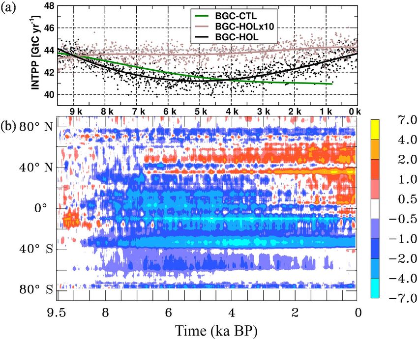
3244                                                         J. Segschneider et al.: Marine carbon cycle during the Holocene

the marine carbon cycle (e.g. Jungclaus et al., 2010; Brovkin      complexity models with non-accelerated forcing (Renssen
et al., 2010), and more recently the CMIP5/PMIP3 Millen-           et al., 2005, 2009; Blaschek et al., 2015). Longer model
nium experiments (Atwood et al., 2016; Lehner et al., 2015).       simulations also exist for Earth system models of interme-
   Of the many features that characterize the biogeochemical       diate complexity (EMICS), such as described in Brovkin
system in the ocean, here we will concentrate on oxygen min-       et al. (2016) for the last 8 kyr, and for 6 to 0 kyr BP with a
imum zones (OMZs), atmosphere–ocean carbon fluxes, and             comprehensive ocean–atmosphere–land biosphere model but
the marine ecosystem. OMZs have received particular atten-         with orbital forcing only (Fischer and Jungclaus, 2011). The
tion in the recent past. This is in large part due to the obser-   longest non-accelerated climate simulation with a compre-
vation that in the last 5 decades, a general deoxygenation of      hensive model is the Tra-CE 21ka model experiment with
the world’s ocean and an intensification of the ocean’s main       the Climate Community System Model 3 for the last 21 kyr
OMZs have occurred (e.g. Stramma et al., 2008; Karstensen          (Liu et al., 2014).
et al., 2008; Schmidtko et al., 2017). A further decrease in          A second source of information about climate variability
oceanic O2 concentrations has been projected for the future        during the Holocene comes from proxy data. A concerted ef-
with numerical models (e.g. Matear and Hirst, 2003; Cocco          fort to synthesize these estimates by the PAGES2K project
et al., 2013; Bopp et al., 2013) as a consequence of anthro-       has resulted in a temperature reconstruction over the last
pogenic climate change. Knowing the past variations of the         2000 years at a fairly high temporal resolution (PAGES 2k
OMZ extent and oxygen is, therefore, of immediate relevance        Consortium, 2013). In this reconstruction, the global mean
to estimate the importance of the observed and projected de-       surface air temperature is analysed to cool by about 0.3 ◦ C
oxygenation (e.g. Bopp et al., 2017).                              between 1000 and 1900 AD, followed by a sharp increase in
   A few studies that investigate past oxygen variations           temperature. Before 1000 AD the temperature is fairly con-
have already been performed: based on a model study with           stant, at about 0.1 ◦ C colder than the 1961–1990 average.
an intermediate complexity model to investigate glacial–              Wanner et al. (2008) also provide a comprehensive
interglacial variations of oxygen, Schmittner et al. (2007)        overview of the globally collected proxy-based climate evo-
found a causal relationship of Indian and Pacific Ocean            lution for the last 6000 years together with some instructive
oxygen abundance and a shut-down of the Atlantic Merid-            plots of the insolation changes during that period based on
ional Overturning Circulation (AMOC). In their experi-             Laskar et al. (2004). For land-based proxies the authors con-
ments, AMOC variability was generated by freshwater per-           sistently find a decrease in temperatures from 6 kyr BP until
turbations. An attempt to better understand the currently ob-      now, with different amplitude, but for the ocean this is more
served and future projected expansion of the OMZ based on          heterogenous (Wanner et al., 2008, Fig. 2). For example, the
paleo-oceanographic observations (Moffitt et al., 2015) indi-      sea surface temperature (SST) displays an increase with time
cates an expansion of the major OMZs in the world ocean            in the subtropical Atlantic, whereas SST decreases in line
concurrent with the warming since the last deglaciation (18–       with the land surface records in the western Pacific and in
11 kyr BP, kilo years before present). This is based on esti-      the North Atlantic (see also Marchal et al., 2002).
mates of seafloor deoxygenation using snapshots at 18, 13,            A continuous reconstruction of temperatures for the entire
10, and 4 kyr BP. Bopp et al. (2017) investigated oxygen vari-     Holocene, i.e. the past 11 300 years, albeit with lower tempo-
ability from the last glacial maximum (LGM) into the future        ral resolution before the PAGES2K period, has been assem-
based on CMIP5 simulations (PiControl, the historical and          bled by Marcott et al. (2013). In their reconstruction, global
future periods) and time-slice simulations of the last LGM         mean surface air temperature increases by about 0.6 ◦ C be-
(21 kyr BP) and the mid-Holocene (6 kyr BP).                       tween 11.3 and 9 kyr BP to 0.4 ◦ C warmer than present (as
   Although the focus of this paper is on marine biogeo-           defined by the 1961–1990 CE mean). After 6 kyr BP temper-
chemistry, it is mainly the changes in climate that are driv-      atures slowly decrease by 0.4 ◦ C until 2 kyr BP and are rela-
ing the changes in marine biogeochemistry. Hence, some             tively stable for 1000 years. This is followed by a relatively
characteristics of the Holocene climate variability need to        fast decrease beginning around 1 kyr BP of 0.3 ◦ C, in agree-
be addressed. Model-based investigations of Holocene cli-          ment with the PAGES2K data and an increase to present-
mate are performed under the auspices of the Paleo Model           day temperatures in the last few hundred years before present
Intercomparison Project (PMIP, Braconnot et al., 2012). Ini-       (Marcott et al., 2013, Fig. 1a–f).
tially, numerical model time-slice experiments were used              Model simulations and proxy-based estimates of past cli-
to simulate the climate at specific time intervals, typically      mate variability apparently show some disagreement (Liu
9.5 kyr, 6 kyr, and 0 kyr BP. The simulated climate and its        et al., 2014), and the model simulations described here make
variability have been compared to proxy data (e.g. Leduc           no exception. One reason may be a different behaviour of
et al., 2010; Emile-Geay et al., 2016). Also, transient ex-        land and ocean, as e.g. the PMIP2 model simulations in Wan-
periments over the entire Holocene have been performed,            ner et al. (2008) show warmer mid-Holocene temperatures
mainly with accelerated orbital forcing to save computing          over land, in particular over Eurasia, whereas there is little
time (Lorenz and Lohmann, 2004; Varma et al., 2012; Jin            SST difference between 6 kyr BP and modern values. Also,
et al., 2014), or coupled atmosphere–ocean intermediate            on shorter timescales there are discrepancies between model

Biogeosciences, 15, 3243–3266, 2018                                                    www.biogeosciences.net/15/3243/2018/
J. Segschneider et al.: Marine carbon cycle during the Holocene                                                           3245

results and proxy-based records. For example, proxy-based         in Sect. 2, report the results for climatic and biogeochemical
estimates indicate changing El Niño–Southern Oscillation          variables in Sect. 3, and discuss the results and implications
(ENSO) related variability during the Holocene that cannot        for future research in Sect. 4.
be reproduced by most of the PMIP models (Emile-Geay
et al., 2016). Also, the proxy-derived inverse relationship be-
tween ENSO variability and the amplitude of the seasonal          2     Model description and experiment set-up
cycle is not picked up by most of the models (Emile-Geay
et al., 2016, Fig. 3). The reasons for the mismatch in proxy-     2.1     Models
based and model-simulated Holocene climate variability, de-
                                                                  2.1.1    The Kiel Climate Model (KCM)
spite some efforts in the PMIP community, have yet to be
established.                                                      Oceanic physical conditions are obtained from the KCM
   In this paper we aim at closing the gap between glacial–       (the Kiel Climate Model, Park and Latif, 2008; Park et al.,
interglacial and future greenhouse gas (GHG) driven simula-       2009) a global coupled climate model, in particular from
tions of climate and the marine carbon cycle and earlier time-    NEMO/OPA9 (Madec, 2008), which comprises the oceanic
slice experiments of the Holocene. Given the differences          component of KCM and includes the LIM2 sea-ice model
in simulated and proxy-derived climate evolution over the         (Fichefet and Morales Maqueda, 1997). The atmospheric
Holocene, this study should be regarded as a sensitivity study    component is ECHAM5 (Roeckner et al., 2003). The spa-
to orbital and GHG forcing. Following earlier time-slice ex-      tial configuration for ECHAM5 is T31L19, and for NEMO
periments with a coupled atmosphere–ocean–sea-ice climate         the ORCA2 configuration is chosen, i.e. a tripolar grid with
model and a marine biogeochemistry model (Xu et al., 2015),       a nominal resolution of 2◦ × 2◦ and a meridional refinement
here we use transient model simulations with a comprehen-         to 0.5◦ near the Equator and 31 layers with a finer resolution
sive model system that cover the last 9.5 kyr of the Holocene.    in the upper water column. The upper 100 m are resolved by
In particular, we investigate the temporal evolution of some      10 layers, and below the euphotic zone there are 20 layers
of the key elements of the simulated climate that are im-         with increasing thickness up to a maximum of 500 m for the
portant drivers of marine biogeochemistry variations, such        deepest layer.
as SST and AMOC. For the marine carbon cycle we focus                KCM has previously been used to conduct and anal-
on global values of primary production, export production,        yse time-slice simulations of the pre-industrial and mid-
and calcite export, all of which can result in atmosphere–        Holocene climate and hydrological cycle (Schneider et al.,
ocean CO2 flux and OMZ variations. Based on these results         2010; Khon et al., 2010, 2012; Salau et al., 2012) and con-
we analyse and discuss changes in the OMZs, in particular         tributed to PMIP3 (e.g. Emile-Geay et al., 2016). More re-
in the eastern equatorial Pacific (EEP) but also in the At-       cently, orbital forcing (eccentricity, obliquity, and preces-
lantic and the Arabian Sea, the integrated effect of changes in   sion) were varied continuously over the last 9500 years of the
the atmosphere–ocean CO2 flux, and changes in the marine          Holocene according to the standard protocol of PMIP (Bra-
ecosystem.                                                        connot et al., 2008). This forcing was accelerated by a factor
   In addition we want to address the more technical ques-        of 10, resulting in a transient model experiment of 950 model
tion to what extent simulations with accelerated orbital forc-    years for the Holocene (Jin et al., 2014). Here, in additional
ing are suitable for Holocene marine biogeochemistry sim-         KCM experiments, the forcing is non-accelerated, so that the
ulations. In the accelerated-forcing experiments, the change      Holocene is represented by 9500 model years starting from
in orbital parameters between 2 model years corresponds to        9.5 kyr BP (see Sect. 2.2.1 for the experiment description).
a 10-year step in the real orbital forcing (see Sect. 2.2.1).
For climate simulations, the sensitivity to accelerated vs.       2.1.2    Pelagic Interactions Scheme for Carbon and
non-accelerated forcing has recently been investigated for                 Ecosystem Studies (PISCES)
the last two interglacials (130–120 and 9–2 kyr BP, Varma
et al., 2016), indicating that non-accelerated experiments dif-   Monthly mean fields of temperature, salinity, and the velocity
fer from accelerated experiments in the representation of         from the KCM experiment were used in offline mode to force
Holocene climate variability at the higher latitudes of both      a global model of the marine biogeochemistry (PISCES, Au-
hemispheres, while the behaviour is more similar at low lat-      mont et al., 2003).
itudes. A different temporal evolution was also found for            Since the description of PISCES in Aumont et al. (2003)
the deep ocean temperature, with the non-accelerated exper-       is quite comprehensive, we restrict the model description
iment displaying a larger variation. Here we perform and          to the most relevant parts for our investigation. Sources of
analyse simulations of the marine biogeochemistry of the          oceanic oxygen are gas exchange with the atmosphere at
Holocene forced by an accelerated and a non-accelerated cli-      the surface, and biological production in the euphotic zone.
mate model simulation of the Holocene.                            Oxygen-consuming heterotrophic aerobic remineralization
   We will first describe the numerical models, the experi-       of dissolved organic carbon (DOC) and particulate organic
ment set-up, and characteristics of the time-varying forcing      carbon (POC) is simulated over the whole water column, i.e.

www.biogeosciences.net/15/3243/2018/                                                    Biogeosciences, 15, 3243–3266, 2018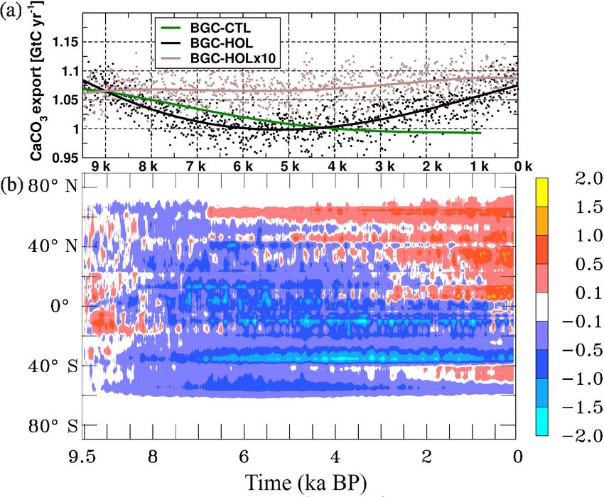
3246                                                         J. Segschneider et al.: Marine carbon cycle during the Holocene

also in the euphotic layer. Remineralization depends on local      into account changes in total solar irradiance (TSI), sea level,
temperature and O2 concentration. For an increase of 10 ◦ C        changes in ice sheets (neither topography nor albedo), fresh-
the rate increases by a factor of 1.8 (Q10 = 1.8). Remineral-      water input into the North Atlantic, or volcanic aerosols.
ization is reduced for O2 concentrations below 6 µmol L−1 .           Greenhouse gas concentrations were obtained from
   Primary production is simulated by two phytoplank-              the PMIP database (https://www.paleo.bristol.ac.uk/~ggdjl/
ton groups representing nanophytoplankton and diatoms.             pmip/pmip_hol_lig_gases.txt; last access: 22 May 2018)
Growth rates are based on temperature, the availability of         based on ice cores from the EPICA site (Augustin et al.,
light, the nutrients P and N (both as nitrate and ammonium),       2004) and are displayed in Fig. 1a). Prescribed atmospheric
Si (for diatoms), and the micronutrient Fe. The elemental ra-      CO2 concentration varied from 263.7 ppm at the beginning
tios of iron, chlorophyll, and silicate within diatoms are com-    of the Holocene, decreased to 260 ppm around 7 kyr BP in
puted prognostically based on the surrounding water’s con-         the mid-Holocene, and then increased to about 274 ppm
centration of nutrients. Otherwise elemental ratios are con-       for the present-day pre-industrial conditions (based on In-
stant following the Redfield ratios. Photosynthetically avail-     dermühle et al., 1999). CH4 varied from 678.8 ppb in the
able radiation (PAR) is computed from the short-wave radi-         early Holocene to 580 ppb around 5 kyr BP, slowly increas-
ation passed from ECHAM to NEMO. Sea ice is assumed                ing afterwards to 650 ppb around 0.5 kyr BP, followed by
to reflect all incoming radiation, so there is no biological       a steeper increase to 805 ppb during the last 500 years of
production in areas that are completely sea-ice-covered (i.e.      the Holocene, reflecting early land-use change. N2 O varia-
where the sea-ice fraction is equal to 1).                         tions were smaller, from 260.6 ppb in the early Holocene to
   There are three non-living components of organic carbon         267 ppb around 2.5 kyr BP.
in PISCES: semi-labile DOC, as well as large and small                Eccentricity remained fairly constant at a value of 0.02
POC, which are fuelled by mortality, aggregation, fecal pellet     over the entire Holocene. The precessional index increased
production, and grazing. In the standard version of PISCES,        from −0.015 to 0.02, and the obliquity decreased from about
large and small POC sinks to the sea floor at respective set-      24.2 to 23.5◦ . In general, this leads to less insolation during
tling velocities of 2 and 50 m d−1 . For large POC, the set-       Northern Hemisphere summer and more insolation in South-
tling velocity increases further with depth. In the model ver-     ern Hemisphere summer: solar radiation at the top of the
sion employed here, the simulation of the settling velocity of     atmosphere (TOA) in June decreased during the Holocene
large detritus is formulated, allowing for the ballast effect of   from 9.5 to 0 kyr BP by about 25 Wm−2 at the Equator, and
calcite and opal shells according to Gehlen et al. (2006). The     45 Wm−2 at 60◦ N. In the Southern Hemisphere, the de-
settling velocity of small POC remains constant at 2 m d−1 .       crease is up to 10 Wm−2 at 30◦ S, and at 60◦ S there is a
In most areas and at most depths, the ballast parameteriza-        weak increase of a few Wm−2 . In December the insolation is
tion leads to a reduction of the settling velocity for large POC   stronger for 0 kyr BP than for 9.5 kyr BP by up to 30 Wm−2 at
compared to the (50 m d−1 and more) standard version. The          30◦ S and about 5 Wm−2 at 60◦ N. See also Jin et al. (2014,
new formulation of the settling velocity for large POC gener-      Fig. 2) and Wanner et al. (2008, Fig. 6) for changes in so-
ally improved the oxygen fields of the KCM-driven PISCES           lar radiation at the top of the atmosphere vs. time for differ-
simulation when compared to modern-day WOA data (Gar-              ent latitudes and summer/winter, based on Berger and Loutre
cia et al., 2013), in particular in the EEP (see Appendix A        (1991) and Laskar et al. (2004), respectively.
for a comparison of observed and simulated oxygen distribu-           We note that the total annual radiation driven by preces-
tions and a sensitivity of the OMZ volume to the O2 thresh-        sion changes remains fairly constant at each latitude and
old). Note that the ballast parameterization was not part of       globally, whereas obliquity changes cause changes also in the
the PISCES version used in Xu et al. (2015), and therefore         annual mean insolation (see e.g. Fig.1b in Schneider et al.,
the mean state of the EEP OMZ differs between the experi-          2010). These annual mean changes in TOA insolation from
ments of Xu et al. (2015) and the ones described here.             9.5 to 0 kyr BP are a decrease of around 5 Wm−2 at the poles
   We also added an age tracer to PISCES. The age tracer is        and an increase of 1 Wm−2 at the Equator, thereby poten-
set to zero at surface grid points, and then the age increases     tially increasing the latitudinal temperature gradient.
with model time elsewhere. Advection and mixing are also              For our analyses that focus on ocean physical conditions
applied to the age tracer.                                         and marine biogeochemistry, however, we need to consider
                                                                   the TOA forcing as filtered by the atmosphere, i.e. at the
2.2     Experiment set-up                                          sea surface. In Fig. 1b annual and zonal mean anomalies of
                                                                   short-wave radiation (SWR) at the ocean and sea-ice surface
2.2.1    KCM – greenhouse gases and astronomical                   are displayed as a Hovmöller diagram. These annual mean
         forcing                                                   anomalies are somewhat different from the TOA anomalies,
                                                                   but more relevant for understanding the simulated SST evo-
As GHG and orbital forcing are the boundary conditions             lution and changes in PAR. In the early Holocene, negative
driving the forced variations in the KCM experiments, we           anomalies of −1 to −3 Wm−2 develop at high latitudes of
describe this forcing in a little more detail. We do not take      mainly the Southern Hemisphere. In the mid-Holocene neg-

Biogeosciences, 15, 3243–3266, 2018                                                     www.biogeosciences.net/15/3243/2018/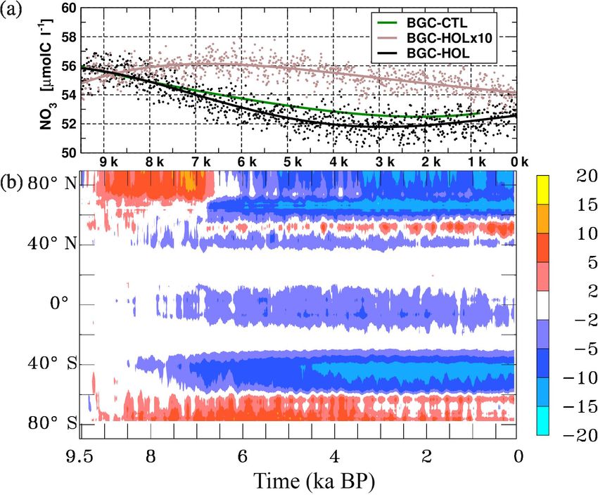
J. Segschneider et al.: Marine carbon cycle during the Holocene                                                                   3247

                                                                       (950 years) and KCM-HOL (9500 years), time-varying
                                                                       orbital parameters and greenhouse gases as described in
                                                                       Sect. 2.2.1 were applied as forcing.

                                                                       2.2.3    Spin-up of PISCES and control experiment
                                                                                (BGC-CTL)

                                                                       To spin up the biogeochemical model, monthly mean ocean
                                                                       model output from experiment KCM-CTL was used as
                                                                       forcing. This then available 2000-year long forcing (first
                                                                       2000 years of KCM-CTL) was repeated three times to spin
                                                                       up PISCES for 6000 years, after which period the model drift
                                                                       as defined by air–sea carbon flux and age of water masses
                                                                       was negligible. It was in particular the age tracer in the deep
                                                                       North Pacific that required the long spin-up time. Note that
                                                                       this BGC spin-up simulation does not achieve a “classical”
                                                                       time-invariant steady state but reflects the internal variability
Figure 1. Forcing for the KCM-HOL and BGC-HOL experi-                  of the first 2000 years from experiment KCM-CTL and any
ments: (a) Holocene atmospheric greenhouse gas concentrations          remaining drift. After repeating the KCM-CTL forcing three
(CO2 , ppm; CH4 and N2 O, ppb) derived from EPICA ice cores (Au-
                                                                       times for the spin-up, PISCES was integrated for a further
gustin et al., 2004) and provided by PMIP and (b) short-wave radia-
tive forcing at the sea/sea-ice surface in W m−2 for the BGC-HOL
                                                                       8700 years with the available KCM-CTL forcing as a control
experiment as computed in experiment KCM-HOL (i.e. the astro-          experiment for the marine biogeochemistry (BGC-CTL).
nomical TOA changes over the Holocene as shown in Jin et al.,
2014 filtered by ECHAM5, the atmospheric component of KCM).            2.2.4    Transient experiments with PISCES
Hovmöller diagram of the anomaly of zonal and annual means since                (BGC-HOLx10, BGC-HOL)
9.5 kyr BP as a 50-year running mean. Anomalies are derived by
subtracting the average over the first 20 years from the annual mean   Similarly to the set-up of the Holocene KCM experiments,
values.                                                                we performed two transient experiments with PISCES in
                                                                       offline mode. Both transient experiments are also started
                                                                       from year 6000 of the PISCES spin-up experiment. In
ative anomalies of −1 to −3 Wm−2 start to evolve also at               the accelerated experiment BGC-HOLx10, oceanic fields
northern high latitudes, and are −3 to −5 Wm−2 at the south-           of KCM-HOLx10 and the same atmospheric pCO2 as in
ern high latitudes around 60◦ S, whereas SWR anomalies                 KCM-HOLx10 are prescribed as forcing. In this experiment,
become positive at low latitudes (1 to 3 Wm−2 ). At around             PISCES is integrated for 950 years corresponding to the pe-
60◦ N, there is a shift from negative to positive anomalies            riod 9.5 kyr BP to 0 kyr, with 10-fold accelerated forcing.
at around 6.8 kyr BP. During the late Holocene, the posi-              Monthly mean output is stored. The non-accelerated exper-
tive anomalies at the low latitudes intensify (3 to 5 Wm−2 ),          iment BGC-HOL is integrated for 9500 years forced by the
whereas the high-latitude anomalies remain about constant.             non-accelerated experiment KCM-HOL and the correspond-
                                                                       ing pCO2 . All experiments and their names are summarized
2.2.2   KCM experiments (KCM-CTL, KCM-HOLx10                           in Table 1.
        and KCM-HOL)                                                      Note that the approach here differs from earlier work to
                                                                       investigate Holocene OMZ changes with a KCM/PISCES
The basis for the KCM experiments is a 1000-year KCM                   model set-up, where PISCES was forced by PMIP-protocol
experiment with 9.5 kyr BP orbital parameters, 286.6 ppm               time-averaged oceanic conditions for specific time slices
CO2 , 805 ppb CH4 , and 276 ppb N2 O concentration (with               (6 and 0 kyr BP, Xu et al., 2015). Also, now all BGC ex-
a final global average SST of 15.8 ◦ C), followed by a spin-           periments make use of the direct KCM-NEMO output, as
up for a further 1000 years with 9.5 kyr BP orbital and                opposed to the set-up in Xu et al. (2015), where KCM-
9.5 kyr BP GHG forcing (pCO2 = 263.8 ppm, CH4 = 678.8,                 derived anomalies were added to mean ocean fields from a
and N2 O = 260.6 ppb). From this state the KCM-CTL                     reanalysis-forced ocean-only set-up.
and KCM-HOL experiments were started. The KCM con-
trol experiment (KCM-CTL) was integrated for a further                 2.3     Processing of model output
8700 years with orbital parameters and atmospheric green-
house gases kept constant at 9.5 kyr BP values as a con-               All plots in the results section are based on model output in-
tinuation of the spin-up experiment. Due to computational              terpolated to a regular 1◦ × 1◦ grid using the CDO/SCRIP
limitations, it was not possible to run KCM-CTL for the                interpolation package. The only exception is the meridional
full 9500 years. In transient experiments KCM-HOLx10                   overturning circulation (MOC) that has been computed on

www.biogeosciences.net/15/3243/2018/                                                          Biogeosciences, 15, 3243–3266, 2018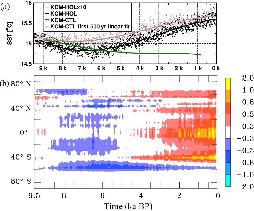
3248                                                             J. Segschneider et al.: Marine carbon cycle during the Holocene

Table 1. Experiment names and characteristics. See also Fig. 1 for the temporal evolution of atmospheric greenhouse gases. Lower entries
in column “forcing exp” indicate the KCM experiments that have been used to force the BGC experiments. (×10) indicates an acceleration
factor of 10. CH4 and N2 O are not prescribed in PISCES.

                  Experiment           Model    orbit (kyr BP)     pCO2 (ppm)       pCH4 (ppb)       pN2 O (ppb)       model
                                                 (forcing exp)                                                          years
                  KCM-CTL              KCM                 9.5           263.77           677.88            260.6       8,700
                  KCM-HOLx10           KCM       9.5–0 (×10)       263.77–286.2         575–805           258–268         950
                  KCM-HOL              KCM              9.5–0      263.77–286.2         575–805           258–268        9500
                  BGC-CTL             PISCES     KCM-CTL                 263.77               n/a               n/a     8,700
                  BGC-HOLx10          PISCES   KCM-HOLx10          263.77 -286.2              n/a               n/a       950
                  BGC-HOL             PISCES     KCM-HOL           263.77 -286.2              n/a               n/a     9,500

                n/a: not applicable

the original ORCA2 grid for different ocean basins us-
ing the standard cdf tool available from the NEMO pack-
age (https://github.com/meom-group/CDFTOOLS; last ac-
cess: 22 May 2018). Maximum values have been computed
using the Ferret @max function.
   For all time series the time axis represents the forc-
ing years. This corresponds to model years for the non-
accelerated experiments but not for the accelerated experi-
ments, so any variation caused by long-term internal vari-
ability of the model would be spread out in time in the accel-
erated experiment compared to the non-accelerated experi-
ment. For all time series, the long-term changes are indicated
by the fourth-order polynomial fits from the Grace software
package (http://plasma-gate.weizmann.ac.il/Grace/; last ac-
cess: 22 May 2018). An exception is alkalinity, where poly-
nomial fits are of the eighth order to allow for the higher
curvature of the time series. Dots represent annual averages
and their spread indicates interannual to centennial timescale
variability. Plots for BGC-HOL and BGC-CTL are based on                 Figure 2. (a) Time series of annual and global mean SST in ◦ C for
                                                                        the three KCM experiments KCM-HOL (non-accelerated forcing,
output from every tenth year, both to be consistent with BGC-
                                                                        black), KCM-HOLx10 (10 times accelerated forcing, brown), and
HOLx10 and to keep the output file size at a manageable
                                                                        control experiment KCM-CTL (green). Circles represent annual av-
level.                                                                  erages (not every year shown), solid lines a fourth-order polynomial
                                                                        fit. The bold grey line indicates a linear fit over the first 500 years of
                                                                        experiment KCM-CTL. (b) Hovmöller diagram of the zonal mean
3     Results                                                           SST anomaly in ◦ C for KCM-HOL, computed by subtracting the
                                                                        average over the first 20 years of KCM-HOL from annual mean
3.1     Climate variations over the Holocene                            values and smoothed by a 10-year running mean. See the colour bar
                                                                        for contour intervals.
Since the biogeochemical variations depend to a large extent
on the changes in ocean physics, we will first examine the
relevant aspects of the simulated climate variations over the
Holocene.                                                               fits). In KCM-HOLx10, the temporal evolution is similar to
                                                                        that in KCM-HOL, but with a smaller decrease in global
3.1.1    Sea surface temperature                                        mean SST in the early Holocene (to 15.0 ◦ C) and a slightly
                                                                        higher SST than KCM-HOL at the end of the late Holocene
As a first indicator of simulated changes in ocean physics,             (15.7 ◦ C).
we present time series of the global and annual mean SST                   Also, the KCM-CTL control experiment displays a de-
(Fig. 2a). The global mean SST in KCM-HOL is 15.1 ◦ C at                crease in global mean SST of about 0.1 ◦ C per 1000 years
9.5 kyr BP, decreases to 14.8 ◦ C at 6.5 kyr BP, and increases          over its first 3500-year integration time. This drift reduces
to 15.6 ◦ C at 0 kyr BP (based on fourth-order polynomial               to 0.1 ◦ C per 2000 years between 6 kyr and 4 kyr BP, and af-

Biogeosciences, 15, 3243–3266, 2018                                                             www.biogeosciences.net/15/3243/2018/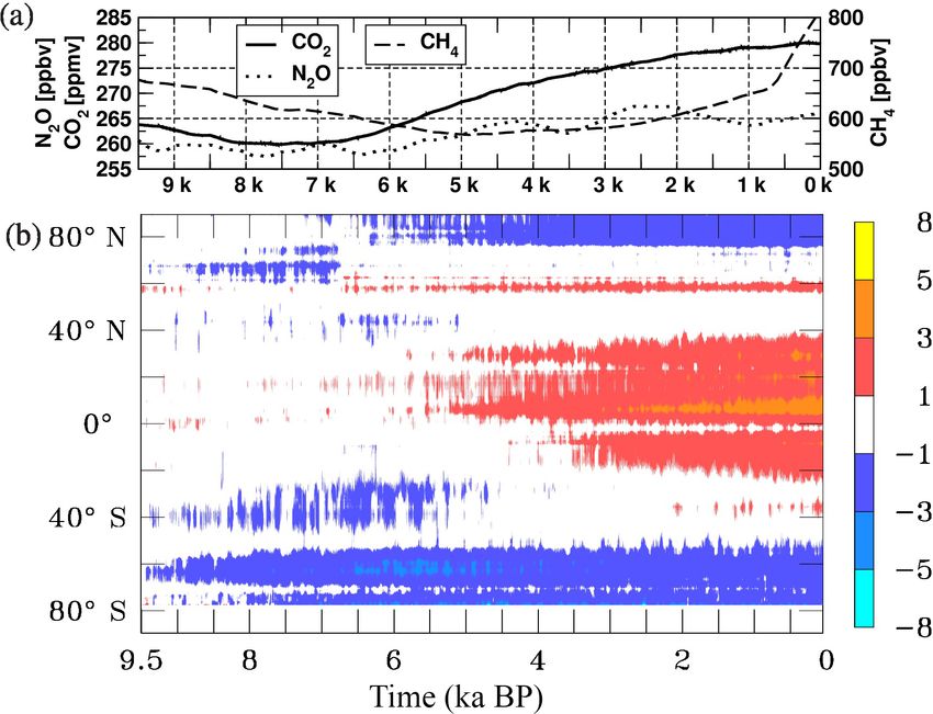
J. Segschneider et al.: Marine carbon cycle during the Holocene                                                                          3249

Figure 3. As in Fig. 2a but for the maximum meridional overturning
circulation in the Atlantic at 30◦ N (solid lines, left axis) and for the
deep Pacific between 3000 m and 5000 m depth at 0◦ N (dashed line,
right axis) in Sv (106 m3 s−1 ).

ter 4 kyr BP the drift becomes very small. Note that the drift
over the first 500 years is negligible in KCM-CTL (grey bar
in Fig. 2a). That even a 500-year period of stable SST does
not guarantee a later drift-free climate in the control simula-
                                                                            Figure 4. (a) Idealized age (time since contact with the surface)
tion is rather unexpected.                                                  in years averaged over a volume in the deep North Atlantic (40◦ W–
   The SST evolution in KCM-CTL implies that the sim-                       10◦ E, 40–60◦ N, 1800–2500 m depth) based on annual mean values
ulated early Holocene decrease in SST in KCM-HOL and                        for KCM-HOL (black), KCM-HOLx10 (brown) and KCM-CTL
KCM-HOLx10 is the combined result of a remaining model                      (green). (b) Change in annual maximum mixed layer depth in me-
drift, and the orbital and CO2 forcing. The initial SST de-                 tres in the North Atlantic between two periods before and after the
crease would be weaker, and the SST increase from the mid-                  shift in water mass age in KCM-HOL (7.8 minus 5.8 kyr BP, mean
to-late Holocene would be stronger in a drift-free experiment               over 200 years centred around the respective dates).
KCM-HOL.
   A Hovmöller diagram of zonal mean SST anomalies of
KCM-HOL (Fig. 2b) reveals that the mid-Holocene cooling                     culation. AMOC then marginally increases until the end of
is strongest at the higher latitudes of the Southern Hemi-                  the Holocene to around 12.6 Sv (Fig. 3).
sphere (up to −0.75 ◦ C, centred at around 60◦ S), whereas                     In KCM-HOLx10 the mean AMOC and its temporal evo-
the late Holocene warming is strongest between 40◦ S and                    lution are similar to KCM-HOL, with a slightly higher mean
40◦ N, with maxima around the Equator and at 40◦ S. This                    value. The KCM-CTL control experiment, however, also dis-
pattern coincides to a large extent with that of the anomalies              plays changes in AMOC, similar to the changes in KCM-
of SWR at the ocean and sea-ice surface (Fig. 1b).                          HOL. Overall, the long-term changes in AMOC are relatively
   The seasonal cycle of global mean SST in KCM-HOL                         small in all experiments and remain within the range of in-
doubles its amplitude from around 0.35 ◦ C in the early                     terannual to centennial variations of around 2–3 Sv.
Holocene to 0.7 ◦ C at about 3 kyr BP (Fig. A3a in the Ap-                     In the Pacific, the deep northward flow that forms the far
pendix), indicating the dominance of the increasing seasonal                end of the deep branch of the conveyor belt circulation also
cycle in the solar forcing on the Southern Hemisphere mid-                  weakens with time during the Holocene. Between 3000 and
latitudes over the decreasing seasonal cycle on the Northern                5000 m depth, at latitude 0◦ N, the decrease in the maximum
Hemisphere (Jin et al., 2014). The seasonal cycle of global                 flow is from almost 10 Sv at 9.5 kyr BP to 7.5 Sv at 0 kyr BP
mean SST remains in the range of slightly less than 0.7 ◦ C                 (dashed line in Fig. 3), indicating a reduced replenishment
during the late Holocene after 3 kyr BP.                                    with younger waters in the deep Pacific. Also, in the Indian
                                                                            Ocean the deep inflow from the south is slightly decreasing
3.1.2    Meridional overturning circulation                                 with time, but less strongly (not shown).

The Atlantic meridional overturning circulation (AMOC)                      3.1.3   Age of water masses
serves as an indicator of the intensity of deep water forma-
tion in the source region of the global conveyor belt. From the             In addition to AMOC, the age of water masses can serve
NEMO-package output, maximum AMOC at 30◦ N has been                         as an indicator of deep water formation and the intensity
computed (Fig. 3). Based on the fourth-order polynomial fits                of the global deep water circulation, and help to under-
shown in Fig. 3, the simulated maximum AMOC at 30◦ N                        stand changes in oxygen concentration. We will investigate
in KCM-HOL at 9.5 kyr BP is around 13.9 Sv. AMOC grad-                      time series of the water mass age in the deep ocean at the
ually decreases to slightly more than 12.5 Sv until 3 kyr BP,               source and end regions of the global conveyor belt circula-
indicating a weak slowdown of the global conveyor belt cir-                 tion, namely the North Atlantic and the North Pacific.

www.biogeosciences.net/15/3243/2018/                                                                Biogeosciences, 15, 3243–3266, 2018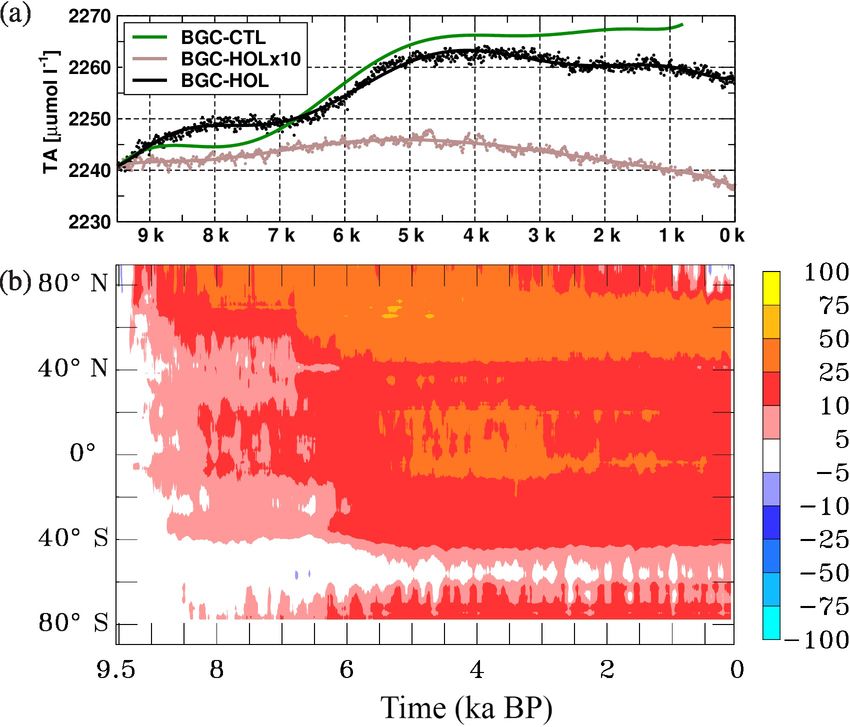
3250 J. Segschneider et al.: Marine carbon cycle during the Holocene
Figure 5. As Fig. 4a, but for the idealized age in years averaged
over a volume in the deep North Pacific (150◦ E–130◦ W, 40–60◦ N,
2500–3500 m depth).
The renewal of water masses in the North Atlantic is
indicated by a time series of the age tracer averaged be-
tween 1800 and 2500 m depth and 40 to 10◦ W, 40 to 60◦ N
in Fig. 4a. The average water mass age in this volume in
BGC-HOL initially ranges from 60 to 80 years over the
first 2800 years, followed by a sudden decrease to slightly
more than 25 years that occurs within a few years around
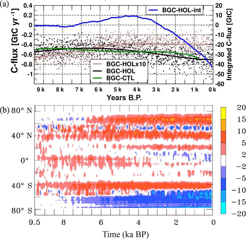
Figure 6. As Fig. 2 but (a) for the global atmosphere–ocean car-
6.8 kyr BP. This is followed by a gradual increase to around bon flux (GtC yr−1 ) of experiments BGC-HOL (black), BGC-
40 years over the remaining 6800 years of the Holocene. The HOLx10 (brown), and BGC-CTL (green), and the integrated
sudden decrease is likely driven by changes in SST in the atmosphere–ocean carbon flux for BGC-HOL (GtC, blue). Negative
North Atlantic which in turn are a consequence of the chang- values indicate oceanic outgassing. The net outgassing of around
ing solar radiation in this area. We will come back to this 0.5 GtC yr−1 balances the river input of carbon. (b) Hovmöller di-
point in Sect. 4.3. agram of the zonal mean atmosphere–ocean carbon flux change
Also, the BGC-CTL control experiment, however, simu- (mol C m−2 s−1 ) of experiment BGC-HOL.
lates a sudden decrease in water mass age similar to the one
in BGC-HOL but occurring at a different time. In the BGC-
HOLx10 (brown curve in Fig. 4a) accelerated experiment a
geochemistry in the Pacific. We will come back to the age of
slightly weaker decrease in age from 60 to 30 years is simu-
water masses when investigating the evolution of the EEP
lated for the deep North Atlantic, but it occurs over a longer
OMZ in Sect. 3.2.5.
time period (roughly 300 model years) and later in terms of
forcing years (between 4 kyr and 1 kyr BP).
At the far end of the conveyor belt circulation, the deep 3.2 Biogeochemical variations
North Pacific, changes occur less suddenly than in the North
Atlantic, but with a larger amplitude. Between 2500 and 3.2.1 Atmosphere–ocean carbon flux
3500 m depth, 150◦ E to 130◦ W, 40 to 60◦ N, the water
masses show an initial age of 1475 years for all experiments In this section the atmosphere–ocean carbon flux is diag-
(Fig. 5). In BGC-HOL, water mass age initially decreases nosed. As atmospheric pCO2 is prescribed in all BGC exper-
to around 1400 years around 7.5 kyr BP, but from then on iments, the diagnosed flux is a combination of the climate-
there is a steady increase up to an age of 1800 years at the driven oceanic variations, and the prescribed pCO2 . We will
end of the Holocene. Also, in BGC-CTL the water mass come back to this point in the discussion (Sect. 4.5).
age in the deep North Pacific increases after 8.5 kyr BP, but In the early Holocene the atmosphere–ocean carbon flux
less strongly than in KCM-HOL. At 0.8 kyr BP, the end of in BGC-HOL is around −0.5 GtC year−1 (Fig. 6a), the equi-
BGC-CTL, the water mass age is 1650 years compared to librium value in the PISCES model, indicating an outgassing
1800 years in KCM-HOL. that balances riverine carbon input. In the mid-Holocene the
This cannot be simulated in the accelerated experiment carbon flux is slightly reduced to around −0.4 GtC yr−1 . In-
BGC-HOLx10, however, which runs for 950 years only. In dicating slightly stronger outgassing, the value increases to
BGC-HOLx10 deep North Pacific water mass age decreases −0.75 GtC yr−1 in the late Holocene in experiment BGC-
to 1400 years at 0 kyr BP. The increase in water mass age in HOL, whereas the flux remains at around −0.4 GtC yr−1
the non-accelerated experiment BGC-HOL indicates a con- in experiment BGC-HOLx10. In BGC-CTL, the CO2 flux
siderable slowdown of the global conveyor belt circulation varies between −0.45 and −0.65 GtC yr−1 . The amplitude
over the Holocene, with significant impact on the marine bio- of the seasonal cycle of the atmosphere–ocean carbon flux
Biogeosciences, 15, 3243–3266, 2018 www.biogeosciences.net/15/3243/2018/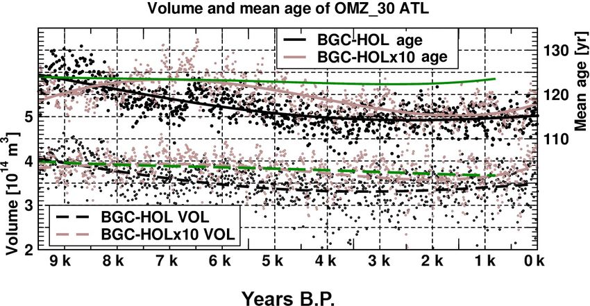
J. Segschneider et al.: Marine carbon cycle during the Holocene                                                                      3251

                                                                        Figure 8. As Fig. 2 but (a) for the average NO3 concentration aver-
Figure 7. As Fig. 2, but for (a) time series of global mean total al-
                                                                        aged over the uppermost 100 m in µmol C L−1 and (b) Hovmöller
kalinity (TA) at the surface in µmol L−1 as eighth-order polynomial
                                                                        diagram of the changes in zonal and annual mean NO3 concentra-
fit, and (b) Hovmöller diagram of the changes in zonal and annual
                                                                        tion in the upper 100 m in µmol C L−1 . For NO3 units divide by
mean surface TA in µmol L−1 .
                                                                        7.6.

in BGC-HOL decreases from early to late Holocene from
around 1.8 to only 0.8 GtC yr−1 (Fig. A3b).
   The time-integrated atmosphere–ocean carbon flux in
BGC-HOL (blue curve in Fig. 6a) is almost zero during the
early Holocene, and increases to 10 GtC from 7 to 4.5 kyr BP.
From 4 to 0 kyr BP there is a steady decrease to −42 GtC, in-
dicating a net flux from the ocean to the atmosphere in the
late Holocene.
   The zonal mean changes in the atmosphere–ocean carbon
flux in BGC-HOL (Fig. 6b) indicate a change from net CO2
uptake to outgassing in the high-latitude Southern Ocean and
mostly increased uptake at northern mid-latitudes. Also, the
positive anomaly around 40◦ S shows stronger uptake from
mid-to-late Holocene.

3.2.2   Surface alkalinity and pH
                                                                        Figure 9. As Fig. 2 but (a) for time series of global primary pro-
In BGC-HOL total alkalinity (TA) at the sea surface in-                 duction integrated over the upper 100 m in GtC yr−1 (INTPP), and
                                                                        (b) Hovmöller diagram of the changes in zonal and annual mean
creases from 2240 to 2250 µmol L−1 until 8 kyr BP and in-
                                                                        INTPP in mol C m−2 s−1 × 10⁸ .
creases further to 2265 µmol L−1 between 6.5 and 4 kyr BP
(Fig. 7a). After 4 kyr BP, TA decreases to 2258 µmol L−1 in
the late Holocene. In experiment BGC-HOLx10 the global                  only partly be explained by a reduction in CaCO3 export that
mean concentration of TA remains in the range of 2240 to                would drive an increase in TA (Sect. 3.2.4, Fig. 11b).
2245 µmol L−1 , with a maximum at around 6 kyr BP. Sur-                    The global and annual mean pH at the surface follows the
prisingly, also in BGC-CTL TA increases considerably and                temporal variations in atmospheric pCO2 and varies only lit-
even slightly more strongly than in BGC-HOL.                            tle during the Holocene, with changes in the range of a few
   The increase in TA in BGC-HOL occurs over most lati-                 hundredths of pH units (8.13–8.16, not shown).
tudes (Fig. 7b), with a stronger increase north of 40◦ N and
around the Equator between 5 and 3 kyr BP, whereas there is
only a small trend around 60◦ S. This temporal evolution can

www.biogeosciences.net/15/3243/2018/                                                            Biogeosciences, 15, 3243–3266, 2018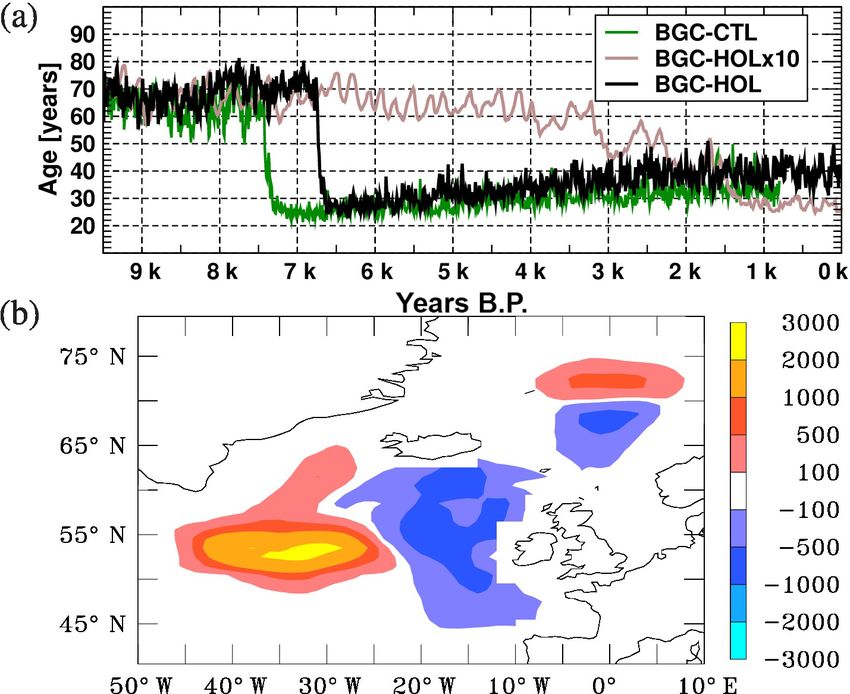
3252 J. Segschneider et al.: Marine carbon cycle during the Holocene
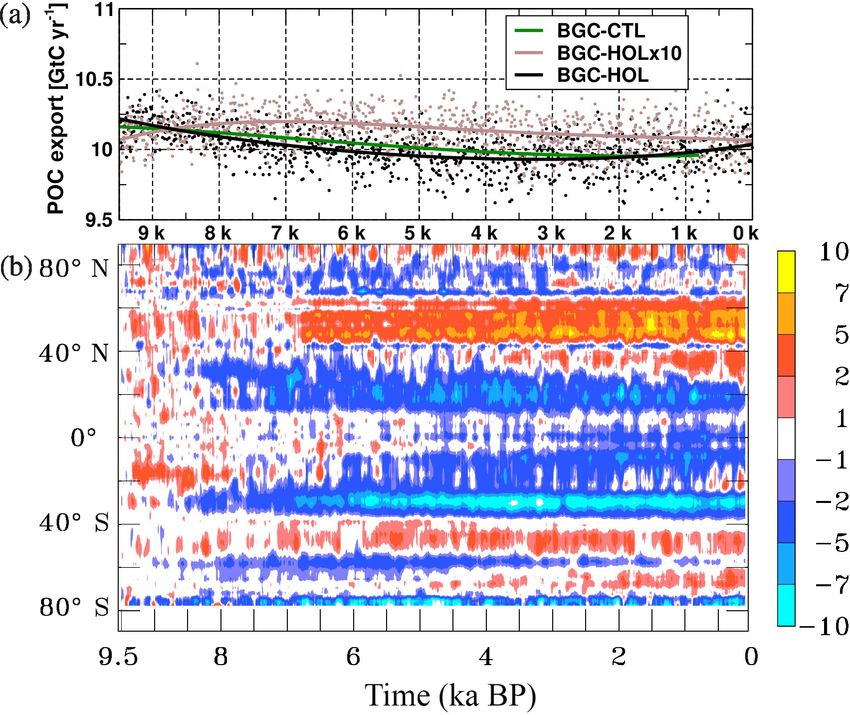
Figure 10. As Fig. 2 but (a) for time series of global export pro- Figure 11. As Fig. 2 but (a) for time series of global CaCO3 export
duction at the bottom of the euphotic layer in GtC yr−1 , and (b) production at the bottom of the euphotic layer in GtC yr−1 , and
Hovmöller diagram of the changes in zonal and annual mean global (b) Hovmöller diagram of change in zonal and annual mean CaCO3
export production in mol C m−2 s−1 × 10⁹ . export in mol C m−2 s−1 × 10⁹ .
3.2.3 Nutrients
sure of the productivity of the marine ecosystem. INTPP
In BGC-HOL, the global mean NO3 concentration aver- in BGC-HOL is around 44 GtC yr−1 at the beginning of the
aged over the euphotic zone (0–100 m) decreases with time Holocene, decreasing to a minimum of around 41 GtC yr−1
from 56 µmol C L−1 in the early Holocene to 52 µmolC L−1 in the mid-Holocene at 5 kyr BP, and then increasing again to
around 3 kyr BP. This is followed by a slight increase 44 GtC yr−1 towards the late Holocene (Fig. 9a). Interannual
to almost 53 µmolC L−1 at 0 kyr BP (Fig. 8a). In BGC- variations are about 2–3 GtC yr−1 . In the accelerated experi-
HOLx10, the global mean concentration is fairly constant at ment BGC-HOLx10, INTPP remains fairly constant over the
56 µmolC L−1 until 5 kyr BP, and then declines gradually to entire Holocene at 43 to 44 GtC yr−1 . In the control experi-
54 µmolC L−1 in the late Holocene. In BGC-CTL, the de- ment BGC-CTL INTPP decreases steadily form 44 to around
crease in the global mean NO3 concentration is similar to 41 GtC yr−1 at the end of the simulation.
that in BGC-HOL until 7 kyr BP, and becomes weaker there- The decrease in global mean INTPP in BGC-HOL orig-
after. inates mainly from latitudes south of 40◦ N and is gener-
The Hovmöller diagram of the zonal mean NO3 concen- ally more pronounced in the Southern Hemisphere (Fig. 9b).
tration changes in experiment BGC-HOL (Fig. 8b) reveals The increase after 4 kyr BP can be traced back to an increase
that the decrease in the NO3 concentration originates from a in INTPP between 40 and 60◦ N beginning around 6 kyr BP
large range of latitudes mainly in the Southern Hemisphere and intensifying and gradually spreading southward for the
(40 to 60◦ S), and also from high northern latitudes after the remainder of the Holocene. This response is likely driven
“event” around 6.8 kyr BP in the North Atlantic centred at by a combination of the changes in SST, PAR, and nutrient
60◦ N. The weak increase in global mean euphotic-zone NO3 availability (Figs. 2b, 1b, 8b), as there is some similarity be-
concentration after 3 kyr BP originates mainly from a small tween zonal mean anomalies of INTPP and SST, SWR at
band centred at 55◦ N, counteracted by a weakening of the the sea/sea-ice surface, and NO3 , but none of the patterns is
negative anomalies around and south of the Equator (10◦ N matched exactly.
to 20◦ S). The export production at 100 m depth in BGC-HOL,
here computed as the sum of small and large POC (see
3.2.4 Marine ecosystem Sect. 2.1.2), is around 10.2 GtC yr−1 at 9.5 kyr BP. Dur-
ing the early and mid-Holocene, there is a slight decrease
Here the focus is on the three major components of the ma- to 9.8 GtC yr−1 at 4 kyr BP, and export production remains
rine ecosystem with relevance for the carbon cycle, namely fairly constant at that level until 3 kyr BP, after which there
the integrated primary production, the export production, and is a modest increase to 10 GtC yr−1 (Fig. 10a). The accel-
the calcite (calcium carbonate) export. The primary produc- erated experiment BGC-HOLx10, after a small increase in
tion integrated over the euphotic zone (INTPP) is a mea- the early Holocene, simulates a relatively uniform decrease
Biogeosciences, 15, 3243–3266, 2018 www.biogeosciences.net/15/3243/2018/J. Segschneider et al.: Marine carbon cycle during the Holocene 3253
Overall the variations of the global marine biological pro-
duction and export rates remain in the range of about 10 %
throughout the Holocene even in the non-accelerated experi-
ment BGC-HOL, with a tendency towards lower values in the
mid-Holocene, and variations surprisingly similar in magni-
tude in the control run.
3.2.5 Oxygen minimum zones
The largest OMZ in the global ocean resides in the EEP.
The EEP here is defined as the region from 140–74◦ W,
Figure 12. Time series of EEP OMZ volume for a threshold of 10◦ S–10◦ N, and to compute the EEP OMZ volume a thresh-
30 µmol L−1 in 1014 m3 (left axis, lower dashed curves) and mean old of 30 µmol L−1 is used. The volume of the EEP OMZ
age of water mass in the EEP OMZ in years (right axis, upper initially remains fairly constant in BGC-HOL from 9.5 to
solid curves). EEP defined as 140–74◦ W, 10◦ S–10◦ N, 0–1000 m 7 kyr BP at 15×1014 m3 (Fig. 12, left y-axis, dashed lines).
depth. Circles represent annual mean values of the OMZ volume, But from 7 kyr BP onwards, the OMZ volume steadily in-
and dots are annual mean values of the water mass age in the EEP
creases to around 26 ×1014 m3 at 0 kyr BP in KCM-HOL, an
OMZ for BGC-HOL (black), BGC-HOLx10 (brown), and BGC-
increase of more than 70 %. In the accelerated forcing exper-
CTL (green). Solid lines represent polynomial fits of fourth order.
iment BGC-HOLx10 the EEP OMZ volume remains fairly
constant over the entire Holocene. Also, in BGC-CTL the
by just 0.1 GtC yr−1 from 8 to 0 kyr BP. Also, control ex- EEP OMZ volume increases after 8 kyr BP, but less strongly
periment BGC-CTL simulates a quite uniform decrease in than in BGC-HOL.
export production, from 10.2 GtC yr−1 at the beginning to At the same time as the OMZ volume increases in BGC-
10.0 GtC yr−1 at the end of the experiment. HOL, the age of the water mass within the OMZ in-
The zonal mean export production in BGC-HOL decreases creases from around 440 years (9.5–7 kyr BP) to 530 years at
mainly at low latitudes in two bands centred around 20◦ N 0 kyr BP (Fig. 12, right y-axis, solid lines). Note that the ac-
and 35 ◦ S (Fig. 10b). An increase occurs mainly between celerated experiment does not show an increase in the OMZ
30 and 60◦ N, intensifying after 6.8 kyr BP. The apparent de- volume and water mass age (Fig. 12). In BGC-HOLx10 the
viations from the pattern of INTPP could be explained by age decreases mainly after 6 kyr BP from 430 to 415 years.
changing temperatures (with an impact on the remineraliza- The longer control run, however, also shows substantial vari-
tion rate) and changes in the particle composition (with an ations of OMZ volume and water mass age. In BGC-CTL the
impact on settling velocity) and relative contributions from water mass age increases to 480 years at the end of the exper-
small and large POC to the export production. For slowly iment, with a slightly stronger increase in the last 2000 years
sinking small POC, we find a more continuous but minor of the experiment.
decline of global export from 3.7 to 3.6 GtC yr−1 , whereas Time series of the oxygen saturation (O2 sat) and apparent
for the faster sinking large POC the decline is more rapid oxygen utilization (AOU) between 100 and 800 m depth in
during the first 3000 years of the Holocene (from 6.5 to the EEP for BGC-HOL demonstrate a relatively stable O2 sat
6.3 GtC yr−1 ) and the export is fairly constant thereafter (not (following mainly the temperature evolution) but an increase
shown). in AOU from 252 to 267 µmol L−1 (Fig. 13a). Late Holocene
The temporal evolution of the calcite export in all experi- minus early Holocene differences show that O2 sat is decreas-
ments is similar to that of INTPP: In BGC-HOL, calcite ex- ing in the upper 400 m of the EEP by up to 5 µmol L−1 , but
port is around 1.08 GtC yr−1 in the early Holocene (Fig. 11a), increasing by up to 4 µmol L−1 below that depth (Fig. 13b,
followed by a decrease of about 0.1 GtC yr−1 (10 %) until shading). The corresponding temperature change is a warm-
the mid-Holocene (around 6 kyr BP) after which there is a ing of up to 0.4 ◦ C in the 100–400 m depth range, and a cool-
slight increase to 1.05 GtC yr−1 towards the late Holocene. In ing of up to 0.4 ◦ C below 400 m depth, with an overall very
BGC-HOLx10 the calcite export fluctuates fairly constantly similar pattern to that of AOU (Fig. 13b, contours).
around its initial value of about 1.08 GtC yr−1 whereas in For AOU, there is a more uniform-with-depth tendency
BGC-CTL an initially stronger decline from 1.075 GtC yr−1 to higher values in the late Holocene, with AOU up to
to slightly less than 1 GtC yr−1 at 0.8 kyr BP is simulated. 25 µmol L−1 higher at around 1000 m depth and slightly
The zonal mean changes in CaCO3 export in BGC-HOL lower late Holocene AOU values only near the surface
are similar to those of INTPP, with an almost global decrease (Fig. 13c, shading). The corresponding change in idealized
in the early Holocene, and a recovery at the higher north- water mass age ranges from 10 to 60 years between 400 and
ern latitudes after 6.8 kyr BP. The recovery gradually ex- 1000 m, with a similar pattern to the AOU changes (Fig. 13c,
tends to the entire Northern Hemisphere in the late Holocene contours).
(Fig. 11b).
www.biogeosciences.net/15/3243/2018/ Biogeosciences, 15, 3243–3266, 20183254 J. Segschneider et al.: Marine carbon cycle during the Holocene
Figure 13. (a) Time series of AOU and O2 sat in the EEP (region as in Fig. 12, but for 100–800 m depth), and (b, c) meridional sections of
zonal mean differences of late Holocene minus early Holocene for (b) O2 sat (shading, µmol L−1 ) and temperature (contours, ◦ C) and (c)
AOU (shading, µmol L−1 ) and water mass age (contours, years). The contour interval for temperature is 0.1 ◦ C from −0.3 to 0.3 ◦ C, with
additional lines for 0.5, 0.7, and 1 ◦ C. The contour interval for water mass age is 10 years from −10 to 60 years, with additional lines at −5
and 5 years. Zero contours are omitted.
In contrast to the EEP, for the OMZ in the tropical At-
lantic mainly south of the Equator, the changes over the
Holocene are more modest and of opposite sign. In the re-
gion from 5◦ W–15◦ E, 30◦ S–5◦ N, the volume of the OMZ
in BGC-HOL decreases slowly from around 4 × 10¹⁴ m3 to
3.5 × 10¹⁴ m3 , and the average age over the OMZ decreases
from about 125 years to 115 years (Fig. 14).
For the Arabian Sea a steady increase in OMZ volume
(here computed for a 70 µmol L−1 threshold) is simulated in
BGC-HOL (1 × 10¹⁴ to 6 × 10¹⁴ m3 ), concurrent with an in-
crease in water mass age from 100 to 120 years (Fig. 15). In
the BGC-HOLx10 accelerated experiment, there is a similar
Figure 14. As Fig. 12 but for the Atlantic in the area of 5◦ W–
15◦ E, 30◦ S–5◦ N, 0–1000 m depth. OMZ volume for a threshold increase in OMZ volume, whereas mean water mass age in-
of 30 µmol L−1 in 1014 m3 and water mass age in years. creases mainly before 6 kyr BP. In BGC-CTL average water
mass age and OMZ volume are much less variable than for
the transient experiments. Note that the results for the Ara-
bian Sea in Gaye et al. (2017) are from an earlier accelerated
experiment, started at year 1500 of KCM-CTL. The earlier
results are quite similar but not identical to BGC-HOLx10.
4 Discussion
4.1 Holocene SST variations
Comparing the KCM-simulated temporal evolution of global
mean SST with observation-based estimates and other model
Figure 15. As Fig. 12 but for the Arabian Sea in the area of 55– simulations, there is a notable difference between models
75◦ E, 8.5–22◦ N, 100–800 m depth. OMZ volume for a threshold and observations. During the proxy-derived climate optimum
of 70 µmol L−1 in 1014 m3 and water mass age in years.
in the mid-Holocene (8 kyr to 5 kyr BP) observation-based
global mean temperature is about 0.4 ◦ C warmer than 1961–
1990 (Marcott et al., 2013), and borehole temperatures from
Export production in the EEP is fairly constant over the Greenland are about 2 ◦ C warmer (Dahl-Jensen et al., 1998).
Holocene at 0.58 GtC a−1 (figure not shown), with only a During the same period the KCM-simulated SST is at its low-
marginal tendency towards lower values in the late Holocene, est value, about 0.8 ◦ C colder than at the end of the simula-
and thus can be ruled out as a driver of the expansion of tion at 0 kyr BP in the non-accelerated experiment (Fig. 2a).
the EEP OMZ. The average O2 concentration within the The largest fraction of the initial post-glacial temperature
OMZ decreases slightly from 18.5 µmol L−1 at 9.5 kyr BP to increase in the reconstructions of Marcott et al. (2013), how-
17.5 µmol L−1 at 0 kyr BP in BGC-HOL (not shown). ever, occurs in the very early Holocene (11.3 to 9 kyr BP),
Biogeosciences, 15, 3243–3266, 2018 www.biogeosciences.net/15/3243/2018/J. Segschneider et al.: Marine carbon cycle during the Holocene 3255
whereas the simulations discussed here start at 9.5 kyr BP to based estimates, however, raises the question of why the sim-
avoid difficulties with the simulation of retreating ice masses ulations result in such a different temporal evolution than
and increasing sea level. Simulations, therefore, start at a observation-based temperature reconstructions.
time when continental ice sheets and sea level are assumed to Possibly there might be a difference in the behaviour of
be close to present-day values. This very early Holocene tem- the SST and the mainly land-based temperature reconstruc-
perature increase can, therefore, not be simulated by KCM tions. For example, Renssen et al. (2009) display simulated
in its present configuration. We note that in the Holocene differences between 9 and 0 kyr BP, and their Fig. 3c sug-
time-slice experiments with KCM, the annual mean SST is gests mainly colder temperatures of the Northern Hemi-
also lowest for the 6 kyr BP experiment and highest for the sphere oceans for 9 kyr BP, whereas the trend is the opposite
0 kyr BP experiment (e.g. Schneider et al., 2010, Fig. 6). for the land surface mainly in Eurasia. Leduc et al. (2010)
In support to our model results, and raising the gen- investigate Mg / Ca ratios and alkenone unsaturation values
eral question of how representative the mainly land based (U37K 0 ) for a range of sediment cores from different loca-
0
proxy-derived temperature anomalies can be transferred to tions. In their study, the majority of the UK 37 records sug-
the Holocene SST, Varma et al. (2016) find a similar temporal gest a Holocene warming trend in the EEP and the tropi-
evolution of global mean SST in their orbitally forced Com- cal Atlantic, whereas Mg / Ca records indicate a Holocene
munity Climate System Model version3 simulations of the cooling trend in the same regions. For the North Atlantic,
Last and Present Interglacials (LIG and PIG, respectively) the alkenone-derived SST decreases over the Holocene, but
mainly in their non-accelerated PIG experiment (their Fig. 4). Mg / Ca-derived SST shows a differing warming/cooling
The larger amplitude of our simulated temperature change trend for the various records. Apparently, further research is
can be explained by the small cooling trend still inherent needed on this issue.
in the control run (KCM-CTL, about 0.1 ◦ C/1000 years, an The model–data mismatch could also imply that at least
otherwise very acceptable value) and the additional forcing early Holocene temperature variations were determined not
from the transient CO2 and CH4 variations in KCM-HOL only by orbital forcing or greenhouse gases, but also by solar
and KCM-HOLx10 with a range of about 20 ppm for CO2 , and volcanic forcing, ice sheets, and internal variability of the
and of about 100 ppb for CH4 (Fig. 1a), whereas Varma et al. system (see also Wanner et al., 2008; Renssen et al., 2009, for
(2016) used constant pCO2 values during their simulations. a more complete and regional investigation of driving mech-
From earlier experiments with KCM with/without a anisms of Holocene climate). However, including total so-
1 %/2 % p.a. atmospheric pCH4 increase a contribution on lar irradiance (TSI) in the forcing would likely not solve the
the order of 0.1◦ C to the simulated Holocene global mean problem. Reconstructed TSI variations over the Holocene are
SST variation from the prescribed CH4 seems a reasonably around 1 W m−2 (Vieira et al., 2011), and assuming a climate
conservative estimate (Biastoch et al., 2011, supplementary sensitivity of 0.5 K (W m−2 )−1 (IPCC, 2007), these could
material Fig. S3). We also performed an additional tran- translate into global mean temperature variations of a sim-
sient non-accelerated KCM experiment with constant pCO2 ilar magnitude to that simulated here, but reconstructed TSI
of 286.4 ppm but orbital forcing for the Holocene that has is relatively low during the mid-Holocene.
not been discussed here. In that experiment, the global mean As proxies might be seasonally biased (e.g. Schneider
SST fluctuates within a constant range almost until 4 kyr BP, et al., 2010), we also analysed the northern summer (June–
i.e. with no mid-Holocene cooling, and increases by 0.2 to July–August, JJA) and northern winter (December–January–
0.3 ◦ C from 4 to 0 kyr BP. This indicates that the early to February, DJF) SST separately, but did not find a better
mid-Holocene SST evolution in KCM-HOL is a result of the match with the proxy-derived mid-Holocene warming. Also,
GHG forcing and any remaining model drift, whereas for the using the yearly maximum temperature, indicating local
late Holocene both GHG and orbital forcing drive an increase summer, does not change the temporal behaviour; it only
in SST. shifts the SST curve upward by roughly 2 K. In summary,
We note that also in the simulations of Varma et al. (2016) the simulated large-scale SST evolution in KCM-HOL is
seemingly small variations in atmospheric pCO2 lead to seemingly not very sensitive to the choice of season. The
larger variations in the simulated global mean SST than ex- Holocene climate conundrum (Liu et al., 2014) is still not
pected from climate sensitivity estimates: For their PIG and solved.
LIG simulations with atmospheric pCO2 of 280 ppm and
272 ppm, respectively, the initial global mean SST difference 4.2 Holocene circulation changes
is more than 0.35 ◦ C. This sensitivity is of similar magnitude
as the 0.6 ◦ C for KCM control simulations with a pCO2 of The meridional overturning in the Atlantic in KCM-HOL de-
286.4 and 263 ppm. creases over the Holocene by about 1.5 Sv/10 %, whereas
As such, the Holocene simulations of Varma et al. (2016) the deep inflow into the Pacific decreases by 2.5 Sv/20 %
and the LGM-to-present simulations discussed in Liu et al. (Sect. 3.1.2, Fig. 3). As the slowdown of the circulation in the
(2014) support the results of our simulations as technically deep Pacific in experiment KCM-HOL seems stronger than
sound. The discrepancy between simulated SST, and proxy- one would expect from the decrease in the AMOC, this sug-
www.biogeosciences.net/15/3243/2018/ Biogeosciences, 15, 3243–3266, 2018You can also read