A Goldilocks Theory of Fiscal Policy
←
→
Page content transcription
If your browser does not render page correctly, please read the page content below
A Goldilocks Theory of Fiscal Policy∗

         Atif Mian                   Ludwig Straub                         Amir Sufi
   Princeton & NBER                Harvard & NBER                Chicago Booth & NBER

                                            June 2021

                                            Preliminary

                                              Abstract
         When an economy is close to the zero lower bound on nominal interest rates,
      governments face a trade-off: excessively conservative fiscal policy risks persistently
      low output but aggressive fiscal expansion raises sustainability concerns. This study
      builds a framework of dynamic fiscal policy, showing that there exists a Goldilocks
      zone in which deficits are permanent but not too high, the nominal interest rate on
      government debt ( R) is lower than the economy’s growth rate (G), government debt
      levels can be substantial, and deficits allow the economy to overcome weak demand
      to achieve potential output. The size of the Goldilocks zone can be estimated using
      empirically observed moments in the data, which suggest for the United States that
      government debt to GDP ratios can reach a maximum of about 220% in the Goldilocks
      zone, but the maximum permanent government deficit is only about 2% of GDP. In
      the model, R and G are endogenous to fiscal policy, which disciplines the ability of
      a government to boost deficits even if R < G. The Goldilocks zone is fragile: it can
      vanish in the face of a decline in potential GDP growth, a rise in aggregate demand, or
      a decline in income inequality.

  ∗ We are grateful to Gabriel Chodorow-Reich, Arvind Krishnamurthy, Hanno Lustig, Klaus Masuch,
Ricardo Reis, Larry Summers, Annette Vissing-Jorgensen, and seminar participants at Queens University,
Georgetown University, Harvard, Stanford GSB, and Berkeley Haas. Laurenz DeRosa, Jan Ertl, Pranav Garg,
and Keelan Beirne provided excellent research assistance. Straub appreciates support from the Molly and
Domenic Ferrante Award. Contact info: Mian: (609) 258 6718, atif@princeton.edu; Straub: (617) 496 9188,
ludwigstraub@fas.harvard.edu; Sufi: (773) 702 6148, amir.sufi@chicagobooth.edu

                                                  1
1     Introduction
Advanced economies in recent years have been characterized by sustained proximity to
the zero lower bound on nominal interest rates, which has led some economists to argue
that persistent fiscal deficits may be necessary to generate demand.1 At the same time,
government debt to GDP ratios are at historical highs, leading to concerns about fiscal
sustainability going forward if deficits are not reduced.2 The tension between these views
has triggered an active debate on fiscal policy with important consequences.
    This study proposes a tractable model of fiscal policy that encapsulates the trade-off
highlighted in this debate. The model adds two main features to an otherwise standard de-
terministic representative-agent economy. First, it introduces a preference for government
debt. Such a preference generates a convenience premium on government debt, and the
convenience premium in the model, as in the data, declines as the level of government debt
outstanding rises (e.g., Krishnamurthy and Vissing-Jorgensen 2012). Second, the model
assumes a zero lower bound on nominal interest rates, which allows for the possibility
that persistently weak demand reduces output, inflation, and the nominal growth rate of
the economy. The government’s fiscal policy in the model can add to aggregate demand
through borrowing, but the policy must satisfy the government budget constraint.
    A key insight of the model is that fiscal policy can be excessively conservative, pushing
the economy toward the ZLB with depressed demand. Or fiscal policy can be too aggressive,
raising fiscal sustainability concerns. There is a Goldilocks zone for fiscal policy in between;
this zone represents the set of equilibrium debt and deficit levels in which the government
is able to run deficits that are permanent but not too high; the nominal interest rate on
government debt R is lower than the economy’s nominal growth rate G; government debt
outstanding can be large; and deficits allow the economy to overcome weak demand in
order to achieve its potential.
    An analysis of the Goldilocks zone helps to provide answers to a number of central
questions facing governments today. Does fiscal consolidation threaten to push an economy
toward depressed output at the ZLB? How large can deficits and debt levels be before
departing the Goldilocks zone? Is there a “free lunch” in which a government can raise
    1 This idea can be traced back to Abba Lerner’s “Functional Finance” view, but has recently been articulated

by Blanchard, Tashiro, et al. [2019] in their discussion of policy in Japan: “under current forecasts about the
rest of the Japanese economy, primary deficits may be needed for a long time . . . they are probably the best
tool for maintaining demand and output at potential.”
   2 Among others, the work by Jiang, Lustig, Van Nieuwerburgh, and Xiaolan [2019, 2020a] has raised

questions on how the pricing of government debt can be consistent with the evolution and riskiness of
revenues and expenditures going forward.

                                                       2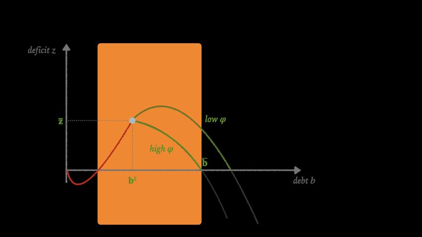
deficits to a higher permanent level without ever having to raise taxes? What underlying
fundamentals of an economy explain the size of the Goldilocks zone, and what changes to
an economy can lead the zone to shrink? Finally, what are the implications of the Goldilocks
zone for tax policy?
    The model addresses the growing body of research seeking to understand the implica-
tions for fiscal policy when the nominal interest rate on government debt is lower than the
nominal growth rate of the economy, R < G. This condition is of central interest because,
as Blanchard [2019] demonstrates, it holds the promise of raising deficits permanently or
temporarily, without ever having to raise taxes. Indeed, we confirm below that assuming
that R and G are exogenous allows a government to sustain arbitrarily large deficits indefi-
nitely as long as R < G. We call a temporary or permanent expansion in deficits a “free
lunch” policy if it is sustainable without a subsequent increase in taxes.
    In our model, R and G are endogenous to fiscal policy, and this has important implica-
tions for whether a free lunch policy is possible. Boosting deficits leads to high debt levels,
which raise interest rates because the convenience premium on government debt declines
when the market is saturated. In contrast, excessively conservative fiscal policy leads to
weak aggregate demand and nominal interest rates being trapped at the zero lower bound,
depressing both real output and nominal growth G. As a result, the condition R < G can be
violated either because debt levels are high and convenience premia low, or because debt
is low with R pinned at zero and G falling below zero due to deflation. The endogeneity
of R and G to government debt levels implies that a simple examination of the difference
between the two at any given point in time is insufficient to understand whether a free
lunch policy is possible or not.
    There is a maximum deficit possible in the Goldilocks zone, and the government debt
level associated with that maximum deficit is crucial in determining whether a free lunch
policy is available. If government debt outstanding is below this threshold, a free lunch
policy is available that allows modest fiscal expansions without ever having to raise taxes.
For example, a free lunch policy always exists for an economy which is at the ZLB. This
helps capture the intuition that governments can safely boost deficits when interest rates
on government debt are close to zero. If debt levels are above this threshold debt level, no
free lunch policy is available, even if R is below G. In this region of the Goldilocks zone,
an increase in deficits has to be met with higher subsequent taxes or reduced deficits. An
economy can be in the Goldilocks zone with R < G and yet be unable to pursue a free
lunch policy.
    The tractability of the model allows for closed form solutions for key determinants

                                              3
of the Goldilocks zone, such as the maximum permanent deficit possible and the largest
amount of government debt for which R remains below G. An advantage of the model is
that the estimation of these important objects is tied directly to empirical evidence from the
macro-finance literature. More specifically, the maximum deficit and debt levels possible in
the Goldilocks zone depend crucially on the sensitivity of the convenience yield, or more
generally of R minus G, to government debt levels.
Using estimates from this literature, we conduct a simple calibration which suggests
that the United States’ Goldilocks zone has a maximum government debt to GDP ratio
of 220%, at which point R rises above G; and a maximum permanent primary deficit of
2% of GDP obtained at the threshold debt level of 110% of GDP. The calibration can easily
be done for any country for which an estimate of the sensitivity of convenience yields to
government debt levels is available, and we provide a range of estimates for Germany,
Italy, and Japan. A general finding from the calibration is that an economy is able to reach
government debt to GDP ratios that are higher than where most advanced economies
currently are before R rises above G, but the maximum possible permanent deficit level is
small relative to the average deficits being run over the past 15 years.
How can the Goldilocks zone be so large? And what changes in the economic envi-
ronment can make it disappear? These questions are of heightened importance given that
government debt to GDP ratios have been high in many advanced economies, exceeding
100% in Belgium (102%), the United States (107%), Portugal (124%), Italy (134%), and Japan
(237%).3
The model shows that the Goldilocks zone is especially large in the presence of weak ag-
gregate demand. The model makes it clear that aggressive fiscal policy allows governments
to treat the symptoms associated with weak aggregate demand. However, this also implies
that the Goldilocks zone can disappear if sustainable aggregate demand returns. When
debt levels are elevated at that point, governments may have to raise taxes by considerable
amounts. The model also highlights that the Goldilocks zone can disappear if the trend
growth rate falls, for example due to demographics or slower productivity growth. In
general, while the Goldilocks zone may exist, it is fragile and can vanish with changes in
the underlying economy.
High income inequality is also an important factor increasing the size of the Goldilocks
zone, which we show by introducing hand-to-mouth agents into the model. High income
inequality allows the government to sustain high debt levels because higher income indi-
viduals in the model, as in the data, hold the majority of the government debt outstanding
3 These are averages from 2015 to 2019.
4in the economy. Hence demand for government debt is higher when income inequality
is higher, thereby lowering the interest rate on government debt. The flipside is also true:
if inequality declines, the Goldilocks zone will shrink and potentially disappear, forcing
the government to run potentially large surpluses. This shows the danger of relying on
aggressive fiscal policy to address challenges to the economy coming from the secular
long-run rise in income inequality. Policies that attempt to reduce inequality in the longer
run may conflict with current policies that boost government deficits, in the sense that an
ultimate decline in inequality will lead to a rise in interest rates forcing the government to
cut deficits in order to pay back the debt that has been accumulated.
The extended model with hand-to-mouth agents also allows for an assessment of tax
policy. An important implication of the model is that redistributive tax policy can make it
harder to finance large deficits. When the government taxes savers, it is taxing the main
holders of government debt, thereby lowering demand for government debt and raising
the interest rate. This presents a challenge: a government cannot simultaneously eliminate
inequality through redistribution and sustain large debt levels at low interest rates. The
model also has implications for the implementation of financial repression and the effects
of tax policy when an economy faces a slowdown in trend growth.
Related Literature. This study is part of a growing body of theoretical research that has
emerged around two important facts on government debt. The first fact is that the nominal
interest rate on government debt is lower than the nominal growth rate on average, R < G
(Feldstein 1976, Bohn 1991, Ball, Elmendorf, and Mankiw 1998, Blanchard 2019, Mehrotra
and Sergeyev 2020). The second, and much more recent fact, is that the demand curve
for government debt slopes down empirically, that is, the interest rate on government
debt rises in the volume of government debt (Krishnamurthy and Vissing-Jorgensen 2012,
Greenwood and Vayanos 2014, Greenwood, Hanson, and Stein 2015). This fact is attributed
to “convenience benefits” of government debt, related to regulatory requirements, premia
for liquidity, and premia for safety.
The literature has explored several ways to explain one or both of these facts. Bohn
[1995] suggests that R < G can naturally occur in complete markets economies with
aggregate risk. Due to Barro [1974] - Ricardian equivalence, the model suggests that
government debt neither affects R, nor can the government run a permanent deficit in each
state of the world. Jiang et al. [2019] demonstrate that this approach cannot explain the
valuation of US government debt. A potential way out is the recent work by Barro [2020]
relying on the risk of rare disasters (Barro and Ursua 2008) that may not have realized yet
5for the US economy. However, the Barro [2020] model is inconsistent with the second fact
above.4
The perhaps largest literature on R < G is based on OLG models, going back to
Samuelson [1958] and Diamond [1965]. An early motivation of this literature has been to
understand when R < G is a sign of dynamic inefficiency (Abel, Mankiw, Summers, and
Zeckhauser 1989, Blanchard and Weil 2001), as well as when a possibility for a “free lunch”
policy exists (Blanchard and Weil 2001, Blanchard 2019), whereby deficits can be increased
today without future tax increases, in any state of the world. Such a policy was found to be
more likely to exist when the economy is inefficient, and when capital is not crowded out.
When a free lunch policy does not exist, deficits resemble a “gamble” (Ball et al. 1998).5
The above facts have also been approached using liquidity premia. Woodford [1990]
illustrates how liquidity demand by producers or consumers can lead to R < G. Angeletos,
Collard, and Dellas [2020] microfound a convenience yield function based on liquidity
needs to revisit the optimality of the Barro [1979] tax smoothing results (see also Canzoneri,
Cumby, and Diba 2016, Bhandari, Evans, Golosov, and Sargent 2017, Azzimonti and Yared
2019). The closest paper to ours among this class of models is Reis [2021]. The paper
microfounds liquidity and safety premia of government debt in an economy with hetero-
geneous savers and producers hit by idiosyncratic productivity shocks. The paper shows
that this economy leads to a “bubble premium” on public debt, defined as the gap between
the marginal product of capital and R, which can be used to sustain permanent primary
surpluses if R < G. Reis [2021] derives several sharp implications of the model, such as
that more government spending reduces R in the model, while greater inequality increases
R. Our analysis complements that of Reis [2021] by exploring a different microfoundation
for why R < G, which is shown to lead to different predictions using a phase diagram
analysis. Moreover, instead of modeling capital and investment, we study the interaction
of R < G with the ZLB.
Mehrotra and Sergeyev [2020] share with our paper the assumption of a convenience
utility function v(b) over government debt in a model with aggregate risk, and allowing for
default risk. Different from Mehrotra and Sergeyev [2020], our focus is on a deterministic
model, which we show can be tractably analyzed using phase diagrams for arbitrary v(b).
We also allow for a ZLB constraint, which we show meaningfully interacts with important
4 We present a model in Section 7.2 that introduces default risk into the Barro [2020] model and shows that
it endogenously generates a “safety premium” for government debt as long as no disaster occurs.
5 Note that in our model, capital would be irrelevant for whether a “free lunch” policy is feasible or not
(which is why we do not include it in our model). This is because the (de-trended) steady-state return on
assets other than government is always equal to the discount rate of agents, irrespective of the steady-state
level of government debt. Therefore, steady-state capital would be independent of the debt level, too.
6comparative statics (e.g. that of falling growth rates).
Our model is based on the assumption that monetary policy remains active in stabilizing
inflation and economic activity whenever it can. A recent branch of the literature explores
deviations from this assumption. Brunnermeier, Merkel, and Sannikov [2020] derive a
Laffer curve for the rate of inflation in a model with liquidity needs among producers.
Sims [2019] argues that fiscal policy should, in general, use this “inflation tax” to generate
seignorage-like revenue and reduce distortionary taxes (different from Chari and Kehoe
1999). The deficit-debt schedule that we derive, and on which our phase diagram is based,
may seem similar to the inflation Laffer curve, but is quite distinct. In our schedule, debt
is on the horizontal axis instead of inflation. With a binding ZLB, we find a positive
relationship between inflation and debt levels, while this branch of the literature generally
finds a negative one. With interest rates above the ZLB, inflation is independent of debt in
our economy.
Finally, this study is closely related to the burgeoning literature on the sources and
implications of safe asset demand (e.g., Caballero, Farhi, and Gourinchas 2008, Caballero
and Farhi 2018, and Farhi and Maggiori 2018). In their model of the international monetary
system, Farhi and Maggiori [2018] explore an equilibrium in which there is large demand
for debt issued by a hegemon government. When this is met by too much issuance, default
risk emerges. Farhi and Maggiori [2018] explain how a zero lower bound constraint can
make this a more likely outcome.
2 Model
We begin with a stylized model that we extend in later sections. The model runs in
continuous time and is deterministic.6 It involves two actors, a government and a represen-
tative household. The government issues government debt, spends, and raises lump-sum
taxes. The representative agent consumes and draws convenience benefits from holding
government debt.
Throughout, we denote by Rt the nominal interest rate on government debt and by
Gt ≡ γ + πt the nominal growth rate, which is equal to real trend growth γ plus inflation
πt . G ∗ ≡ γ + π ∗ corresponds to nominal trend growth, when inflation is at its target π ∗ .
To save on notation, we will conduct our analysis entirely in the context of a model that
6 Aggregate risk is useful to explain the gap between R and G in the data, but it will not affect how R
changes in government debt b, e.g. see the contributions by Bohn [1995] and Barro [2020]. This is why we
focus on a deterministic model for the majority of the paper. In Section 7.2 we extend the Barro [2020] model
with default risk and show that it can micro-found the convenience utility assumed here.
7was de-trended with the nominal growth rate. Potential output y∗ in the de-trended model
is thus constant, and we normalize it to one, y∗ ≡ 1. Any quantities, such as the level of
government debt bt are thus to be understood as government debt relative to potential
GDP. Moreover, we refer to Rt − Gt as the “de-trended rate of return” on government debt,
as it is the return Rt net of the re-investment that is necessary to keep government debt
stable relative to potential GDP.
Households. The economy is populated by a representative household choosing paths
of consumption ct and government debt holdings bt in order to maximize
Z ∞
max e−ρt {log ct + v (bt )} dt (1)
{ct ,bt } 0
subject to the budget constraint
ct + ḃt ≤ ( Rt − Gt ) bt + wt nt − τt . (2)
The objective (1) involves flow utility from consumption log ct and a utility v(bt ) from hold-
ing government debt (relative to potential GDP). The latter captures safety and liquidity
benefits that have been used extensively and are well documented in the literature (e.g.
Sidrauski 1967, Krishnamurthy and Vissing-Jorgensen 2012). In line with this literature,
we assume that the utility over government debt is twice differentiable, increasing and
concave, v0 ≥ 0, v00 ≤ 0.7 Flow utility is discounted using a discount rate ρ. The discount
rate pins down the steady state return on assets other than government debt, which, as we
derive below, is given by ρ + G ∗ .
The budget constraint (2) involves labor income wt nt and lump-sum taxes τt . Labor
income derives from agents selling their labor endowment nt . We assume that agents
wish to sell an endowment of 1 but may be unable to do so due to a standard downward
nominal wage rigidity (which happens at the ZLB in our model). In particular, the path of
nominal wages Wt satisfies
Ẇt
≥ π ∗ − κ (1 − n t ). (3)
Wt
This implies that whenever labor demand is falling short of the unit labor endowment,
wage inflation will fall short of π ∗ . The lower labor demand is, the lower wage inflation
will be, just like in a standard Phillips curve. κ ≥ 0 parameterizes the slope of the Phillips
curve.
7 We also assume that the range of v0 is given by [0, ∞) or (0, ∞) and that v00 < 0 whenever v0 > 0.
8Representative firm. We assume that labor is used by a representative firm with linear
production technology yt = nt . The firm charges flexible prices, pinning down the real
wage wt = 1. Price inflation πt in our de-trended model is equal to wage inflation and
therefore determined by (3).
Government. The government sets fiscal and monetary policy. Fiscal policy consists of
paths { x, bt , τt } of government spending x, government debt bt and taxes τt , subject to the
flow budget constraint
x + ( Rt − Gt ) bt ≤ ḃt + τt (4)
The primary deficit is given by
zt ≡ x − τt (5)
We assume taxes adjust to ensure that zt follows a given fiscal rule zt = Z (bt ). Typically,
Z (b) is downward-sloping in debt b, corresponding to a lower deficits or greater surplus
with higher debt levels.
Government debt bt is short-term and real in our baseline model. We relax both of these
assumptions in Section 7.1. Government spending x ≥ 0 is assumed to be constant for now.
Our analysis below is parallel to one in which government spending is allowed to vary
while taxes are kept fixed (see also Section 6).
Monetary policy is dominant in our model and successfully implements the natural
allocation whenever feasible. In particular, we denote by { R∗t } the path of the nominal
natural interest rate, which would materialize in the absence of nominal rigidities in our
model, assuming inflation is constant at its target π ∗ . We assume that the actual nominal
interest rate then follows
Rt = max{0, R∗t }. (6)
In particular, whenever the natural interest rate is positive, Rt tracks the natural interest
rate R∗t , and the economy is at potential, yt = nt = 1. When the natural rate is negative,
however, Rt is constrained to be equal to zero by the ZLB. In that case, we will find that the
economy falls below potential, yt = nt < 1.8
Equilibrium. We define equilibrium in our model as follows.
Definition 1. Given an initial level of debt b0 and a fiscal rule Z (·), a (competitive) equilib-
rium consists of a tuple {ct , yt , nt , bt , Rt , Gt , πt , τt , zt , wt }, such that: (a) {ct , bt } maximizes
8 This is similar to the rationing equilibria in Barro and Grossman [1971], Malinvaud [1977], and Benassy
[1986].
9the household objective (1) subject to (2); (b) the deficit {zt } follows the fiscal rule Z and
taxes are in line with (5); (c) debt evolves in line with the flow budget constraint (4) and
remains bounded; (d) monetary policy sets the nominal rate Rt in line with the rule (6); (e)
inflation πt is determined by the Phillips curve (3); (f) output yt is given by yt = nt and the
real wage is wt = 1; (g) the goods market clears ct + x = yt . A steady state equilibrium is an
equilibrium in which all quantities and prices are constant.
Stability at the ZLB. One concern with our analysis may be that, when the economy is
at the ZLB, the nominal rate is fixed at zero, Rt = 0. In textbook New-Keynesian (NK)
models, this leads to indeterminacy and thus multiplicity of bounded equilibria (Benhabib,
Schmitt-Grohé, and Uribe 2001, Cochrane 2017). Our model differs from a textbook NK
model in that it involves utility over government debt, which can lead to stability at the ZLB
(Michaillat and Saez 2019). Following a similar logic, one can easily show that equilibria in
our model are locally determinate whenever the Phillips curve is not too steep,
ρ + G∗
κ< . (7)
1−x
We assume that this condition is satisfied for the remainder of our analysis.
Features of government debt in the model The model follows the extensive body of
research arguing that government debt directly enters the utility of those who hold it, which
explains why government debt has low yields relative to similar assets (e.g., Krishnamurthy
and Vissing-Jorgensen 2012, Caballero, Farhi, and Gourinchas 2017). The underlying
logic of this assumption is government debt has certain benefits that lead it to be valued
above and beyond future cash flows. These benefits can be due to primitive factors such
as household demand for liquidity and safety, institutional factors such as regulatory
requirements facing financial institutions, or international factors such as the demand for
dollar-denominated assets.9 Such an assumption generates a convenience yield that helps
9 The demonstration of such a convenience yield on U.S. government debt is the subject of a large
body of research including studies by Krishnamurthy and Vissing-Jorgensen [2012], Vandeweyer [2019],
Van Binsbergen, Diamond, and Grotteria [2019], Koijen and Yogo [2020], Mota [2020]. There is a considerable
range of estimates given in the literature for the size of the convenience yield based on the fact that comparable
assets such as AAA rated bonds may also have a convenience yield. Mota [2020] estimates an average
convenience yield of U.S. Treasuries of 130 basis points. Studies focused on demand for dollar-denominated
debt estimate a convenience yield of U.S. Treasuries of 200 to 215 basis points (e.g., Jiang, Krishnamurthy,
and Lustig [2021], Koijen and Yogo [2020]). Del Negro, Giannone, Giannoni, and Tambalotti [2017] estimated
that rising convenience yields may have been an important factor behind the recent decline of the riskless
rate in the US.
10considerably in explaining the pricing of government debt. For example, of all the potential
solutions to the “U.S. public debt valuation puzzle” considered by Jiang et al. [2019], the
assumption of a convenience yield is the only one that makes a serious dent in the puzzle.
There is a large empirical literature arguing that the pricing advantage of government debt
declines in the amount of government debt outstanding, which is a main feature of our
model. This literature is discussed in detail below in Section 4.2.
An alternative reason for low yields on government debt is that they provide a hedge
against aggregate risk (Bohn 1995), and specifically disaster risk (Barro 2020). These
papers demonstrate that permanent deficits cannot be sustained in every state of the world,
including after disaster shocks. Building on these insights, we provide a microfoundation
of v(b) as “safety premium” in a model with disaster risk and default in Section 7.2 below.
In this microfoundation, disasters occur in different sizes. Debt b is “safe” if it is repaid
after disasters of (almost) all sizes, carrying a large premium. Greater b increases the range
of disasters for which debt is defaulted on, reducing the premium. We show that the
dynamics of this economy before the disaster occurs are isomorphic to those implied by a
model with an exogenous convenience utility v(b).
3 The Goldilocks zone
We begin our equilibrium analysis by studying steady state equilibria.
3.1 Steady state equilibria
Our model admits a set of steady state equilibria, indexed by the level of steady state debt
b ≥ 0. For each b, one can find a primary deficit z such that ḃ = 0 and the economy remains
steady at that level of debt b. We distinguish two cases, according to whether the economy
is above or at the zero lower bound (ZLB).
Above the ZLB. When the economy is above the ZLB, monetary policy implements the
natural allocation. This implies that the interest rate is equal to the natural rate, Rt = R∗t ,
output and employment are at potential, yt = nt = 1, inflation is at its target, πt = π ∗ , and
the nominal growth rate is equal to nominal trend growth, Gt = G ∗ .
To see how the natural rate is determined, consider the household’s Euler equation
ċt
= R∗t − G ∗ − ρ + v0 (bt )ct (8)
ct
11Here, v0 (bt ) enters as it is the marginal convenience utility from saving one more unit in
government bonds. It enters with the opposite sign as the discount rate ρ and therefore
effectively makes the household more patient when saving in government bonds.
In a steady state, consumption is constant and equal to 1 − x by goods market clearing.
This lets us solve (8) for the natural interest rate,
R ∗ ( b ) = ρ + G ∗ − v 0 ( b ) · (1 − x ) . (9)
| {z }
convenience yield
This expression for the natural interest rate on government debt is intuitive. The natural
rate is equal to ρ + G ∗ , which would be the steady state return on any non-convenience-
bearing assets, minus the steady state convenience yield v0 (b) · (1 − x ). The expression
already suggests how R∗ moves with debt. As v is a concave utility function, R∗ weakly
increases in government debt b.
At ZLB. For low levels of government debt b, the natural rate R∗ (b) may be negative
and therefore unattainable for monetary policy due to the ZLB. In this region of the state
space, output falls short of potential and labor is rationed. Using the goods market clearing
condition, output is given by
yt = ct + x (10)
where consumption follows an Euler equation again,
ċt
= 0 − ( G ∗ − κ (1 − yt )) −ρ + v0 (bt )ct (11)
ct | {z }
Rt − Gt
but this time involving a nominal interest rate of zero, Rt = 0, and an endogenous nominal
growth rate Gt = γ + πt with inflation determined by the Phillips curve (3). Solving the
system of (10) and (11) at a steady state with ċt = 0, we find
κ
G (b) = G ∗ − (− R∗ (b)) . (12)
v0 (b) − κ
At the ZLB, the interest rate is exogenous, R = 0, but the nominal growth rate G is
endogenous to the debt level. It lies below nominal trend growth G ∗ , and by more so the
more negative R∗ (b) is. As we show in the appendix, the fraction v0 (bκ)−κ is well defined
with v0 (b) > κ in expression (12) due to our assumption (7).
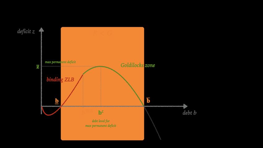
12Figure 1: Nominal interest rates and nominal growth rates across steady state debt levels
3.2 Steady state deficits
Taken together, the previous two sections can be summarized by Figure 1. To explain it, we
go from high to low levels of debt. For high levels of debt, the economy is above the ZLB
and the interest rate R on government debt lies above the growth rate G. As we reduce
debt levels, R falls below G at some b = b and hits the ZLB at some b = b ZLB . At the
ZLB, G starts falling with lower b, as inflation undershoots its target. Eventually, nominal
growth falls below zero due to deflation at b = b. Left of b, R lies above G again.
We can characterize the thresholds in closed form.
Proposition 1. Define
1. b by
1−x
v0 (b)(1 − x ) = ·ρ
1 − x − G ∗ /κ
if 1 − x > G ∗ /κ. Else set b equal to the lower bound of the domain of v0 .
2. b ZLB by
v0 (b ZLB )(1 − x ) = ρ + G ∗
3. b by
v0 (b)(1 − x ) = ρ (13)
Then, b < b ZLB < b. Moreover, R(b) > G (b) iff b < b or b > b, and R(b) = 0 iff b < b ZLB .
13Proposition 1 characterizes the three thresholds that split up the state space into the
four regions shown in Figure 1 according to the relative positions of R(b) and G (b). One
noteworthy implication of the equation for the upper bound (13) is that the size of b can be
large, and is in no meaningful way constrained by existing household or private wealth of
agents. In fact, with ρ → 0, b would diverge to infinity, allowing the government to run
permanent deficits even for very large debt levels. In this limit, private wealth relative to
potential GDP would become unboundedly large. This distinguishes our analysis from
that in Reis [2021], who finds that the level of government debt relative to GDP is bounded
above by the level of private wealth to GDP. There is no such bound in our economy.
An immediate corollary to the proposition is that the gap between the two, G (b) − R(b),
is hump-shaped and positive over the interval (b, b). It peaks right at the point at which
the economy hits the ZLB, b ZLB . This has an important implication for the level of the
primary deficit z(b) that the government is required to choose for the economy to be in a
steady state equilibrium at b,
z(b) = ( G (b) − R(b)) b.
Indeed, the primary deficit is also positive over the interval (b, b). Since G (b) − R(b)
increases for b left of b ZLB , the peak of z(b) must lie weakly to the right of b ZLB . To
characterize the shape of z(b) more formally, we introduce notation to characterize the
semi-elasticity of the convenience yield,
∂v0 (b)
ϕ (b) ≡ −(1 − x ) = −(1 − x )v00 (b)b
∂ log b
We then have the following result.
Proposition 2. The steady state primary deficit is positive over the interval (b, b) and given by
v0 (b)
z ( b ) = v 0 ( b ) · (1 − x ) − ρ b + ( R∗ (b))− b
0
(14)
v (b) − κ
• When the interest rate is at the ZLB, b < b ZLB , the deficit z(b) strictly increases in debt.
• It peaks at b ZLB if ϕ b ZLB > G ∗ /( G ∗ + ρ). In this case, bz = b ZLB .
• It peaks at some bz > b ZLB if ϕ b ZLB < G ∗ /( G ∗ + ρ). In this case bz satisfies
v0 (bz )(1 − x ) = ρ + ϕ(bz ) (15)
14Figure 2: Steady state primary deficits z(b)
(a) Goldilocks zone (b) Goldilocks zone with higher elasticity ϕ
At the peak, the maximum deficit is given by
z = ϕ(bz )bz (16)
Proposition 2 characterizes the shape of steady state primary deficits z(b) as a function
of the debt level b. We sketch the shape in Figure 2. The function z(b) increases when the
ZLB is binding. It stops increasing as soon as the ZLB stops binding if the elasticity of the
convenience yield ϕ b ZLB is higher than G ∗ /( G ∗ + ρ). This ratio corresponds to the ratio
of nominal trend growth to the nominal return on assets other than government debt. With
an elasticity below this ratio, primary deficits keep increasing further, above the ZLB, until
they peak at some debt level bz . As shown in (15) this debt level is greater the smaller the
elasticity of the convenience yield ϕ (bz ) is. The maximum deficit is given by z. Equations
(15) and (16) are implicit equations in general. We solve them below explicitly for special
functional forms of the convenience utility v(b).
However, we already note here that in our model, there is no force that sets a “hard
limit” as to how large the maximum permanent deficit z may be. In fact, as we let the
convenience utility v(b) approximate a linear function of government debt, not only does
b diverge to infinity, so does bz and z with it. In this limit, therefore, there exist steady
states with debt levels and deficits that are many multiples of potential GDP. In practice,
realistic values for the elasticity ϕ may prevent such large deficits and debt levels. This will
be one motivation behind our measurement exercise in Section 4.
153.3 The Goldilocks zone
The steady states with debt levels between b ZLB and b in Figure 2 are situated such that
the interest rate R lies above zero—and hence the economy is above the ZLB—but is not so
large that the economy needs to run a primary surplus, i.e. R < G. We refer to this set of
steady states as the Goldilocks zone.
The Goldilocks zone represents a region of the state space in which the economy
successfully avoids the ZLB on the one side and fiscally unsustainable deficits on the
other. The latter presumes that the economy is able to sustain a steady state with R ≤ G,
or in other words, is able to close any primary deficit. In that case, the Goldilocks zone
corresponds to a “conservative” region of the state space that achieves fiscal sustainability.
Alternatively, if a maximum amount of tax revenue τ is known, that could be used to
derive an upper bound of the primary surplus x − τ. That upper bound could then be used
to describe the upper limit of the Goldilocks zone, in lieu of b. We consider an endogenous
upper bound that is emerging from welfare considerations in Section 7.
3.4 When is rising debt a “free lunch”?
One idea that has garnered considerable attention in the literature surrounding R < G (see,
e.g., Blanchard 2019) is that the condition seemingly allows economies to run larger deficits
temporarily, and then simply “grow out” of the resulting increased debt levels without a
need to raise taxes. We refer to this idea as the “free lunch” property of higher deficits. A
stronger version of the “free lunch” idea is that permanent increases in deficits do not require
tax increases going forward, even if they lead to permanently greater (non-explosive) debt
levels.
Both versions of the free lunch idea can easily be derived from the government budget
constraint (4), under the assumption of a constant interest rate R and a constant growth
rate G > R. Then,
ḃt = − ( G − R) bt + z (17)
describes a stable differential equation for debt b. This implies that temporary increases in
deficits of arbitrary magnitude, leading to greater debt levels, can always be grown out
of over time. Also, a permanent increase in deficits by some ∆z simply raises steady state
debt levels by ∆z/( G − R), with no need for a reduction in deficits, i.e. an increase in taxes,
at any point. Both versions of the free lunch property are satisfied with exogenous R and
G in (17). This is clearly a stylized example but it captures one, if not the most, important
reason why fiscal policy in a world with R < G is thought to be so different from fiscal
16policy with R > G.
We next investigate the extent to which the free lunch idea holds true in our model.
What distinguishes our model from the stylized analysis in (17), is that both G and R are
endogenous to the debt level. To understand the dynamics of bt , it is crucial to incorporate
this endogeneity. To do so, we first describe the behavior of the debt level for a general
exogenous path zt of primary deficits. Then, we feed in the specific paths for deficits that
correspond to the two versions of the free lunch property. We separate again the case at the
ZLB from the case above the ZLB.
Transitions above the ZLB. Above the ZLB, even along transitions, consumption remains
constant at 1 − x. Thus, the natural rate R∗ (bt ) is still given by (9),
R ∗ ( bt ) = ρ + G ∗ − v 0 ( bt ) · ( 1 − x ) .
Therefore, the dynamics of the debt level simplify follow
ḃt = − ( G ∗ − R∗ (bt )) bt + zt (18)
for an exogenous path of deficits zt .10 Notably, the dynamics of debt are perfectly backward
looking, despite households being forward looking with rational expectations. This stems
from the fact that consumption is constant even along transitions due to the goods market
clearing condition, pinning down the natural interest rate in each instant.
Transitions at the ZLB. At the ZLB, the situation is more complex as consumption is no
longer constant. In this case, the economy is described by a system of two differential
equations, the Euler equation
ċt
= − ( G ∗ − κ (1 − x − ct )) − ρ + v0 (bt )ct (19)
ct
in addition to the government budget constraint
ḃt = − ( G ∗ − κ (1 − x − ct )) bt + zt . (20)
Representing transitions in the deficit-debt diagram. A useful diagram to study the
effects of temporary or permanent changes in deficits is the deficit-debt diagram. In
10 If deficits followed a fiscal rule zt = Z (bt ) instead, one would simply have to replace zt in (18).
17Figure 3: Transitions when changing the deficit
Figure 3 we indicate with arrows the direction the economy travels in when deficits are
moved above or below the steady state locus.
The behavior is intuitive. When deficits are raised above the steady state locus, debt
grows, until either the steady state locus is hit, or until, at some point in the future, the
deficit is reduced again down to the steady state locus.When deficits are reduced below
the steady state locus, debt falls over time.
Mathematically, this behavior follows immediately from (18) in the case where the
economy is above the ZLB and the evolution of debt is purely backward looking. In the
case where the economy is at the ZLB, the behavior follows directly from a phase diagram
analysis of (19) and (20).
The free lunch region in our model. The directions in Figure 3 allows us to see the region
of the state space in which the government can obtain a “free lunch”. Indeed, any steady
state on the increasing part to the left of the peak at bz allows for some form of a free lunch.
For example, starting at any of these steady states, a permanent increase in the deficit
to any value below or equal to z can be sustained indefinitely. If the deficit increase is
temporary, it can exceed z, as long as it is reduced back to z or below in time. We show
example transitions along these lines in Figure 4.
An important implication of this behavior of our model is that a free lunch policy is
always available when the interest rate is at the ZLB and b < b ZLB , since the deficit-debt
locus always increases in the ZLB region. This is a result that is often informally made by
18Figure 4: Free lunch (or not)
advocates of “Modern Monetary Theory” (e.g. Kelton 2020). Deficit-financed fiscal stimulus
can always be used to ensure that an economy at the ZLB returns to full employment, and
the resulting increased level of debt need not be repaid by greater tax levels.
However, while the diagram in Figure 4 illustrates how a “free lunch” policy is indeed
possible, it also makes the limits of such a policy very clear. For example, if deficits are
increased by too much and / or for too long, a free lunch cannot obtained.
More fundamentally, a free lunch policy cannot work if the initial debt level already
exceeds bz , that is, the initial steady state lies on the downward-sloping branch of the
deficit-debt locus in Figure 4.11 In this case, any deficit increases, however temporary,
must ultimately be met by reduced deficits, or even, surpluses. In other words, taxes must
increase. Crucially, this logic applies despite the fact that the economy may display R < G
throughout.
How is this possible? The aspect of our theory that is responsible for this result is
the endogeneity of interest rates R∗ (b) to the debt level. As the debt level increases, the
convenience yield of government debt falls, raising the interest cost on all (infra-marginal)
outstanding debt positions. This can undo the positive effect of a greater debt position on
the government budget constraint when R < G that we highlighted at the beginning of this
section. In fact, as Figure 4 illustrates, this precisely happens for debt levels greater than bz .
11 Strictly
speaking, there could be multiple local maxima of z(b) in our model. The condition for the
absence of a free lunch policy is that there be no steady state with a greater debt level and a greater or equal
deficit z.
19This analysis shows that, if the level of debt is larger than bz , the economics behind the
financing of fiscal deficits are entirely conventional: greater debt must be repaid by raising
taxes. Whether R < G or R > G is irrelevant for this question when debt is above bz .
4 Measuring the Goldilocks zone
We have shown in the previous section that the shape of the deficit-debt locus pins down
several key quantities that help us understand the abilities and limits of fiscal policy. In
this section, we set out to calibrate the model to illustrate the key factors determining the
deficit-debt locus, and to offer an attempt to measure the locus as accurately as possible.
Along the way, we focus on three specific quantities that are determined by the deficit-debt
locus: the maximum permanent deficit z, the associated debt level bz , beyond which a free
lunch policy ceases to be feasible, and the level of debt b at which the interest rate R rises
above the growth rate G.
The crucial object to calibrate is the shape of the convenience yield v0 (b)(1 − x ). We
view the fact that v0 (b)(1 − x ) is a crucial object in our model as a promising feature because
there is already a large body of research that seeks to estimate this derivative. We discuss
this literature in detail below.
Our calibration strategy for v0 (b) proceeds in two steps. We first assume a parametric
family of functional forms for v0 (b) and then determine the parameters that match a
given steady state with debt b0 (the US economy in 2019) as well as estimates of the local
(semi-)elasticity of the convenience yield ϕ(b0 ). We henceforth abbreviate ϕ(b0 ) by ϕ.
Since matching the elasticity only provides accuracy in a neighborhood of b0 , we provide
analyses of robustness with respect to the functional forms below.
4.1 Functional forms for the convenience yield
We consider two functional forms for v0 (b) that the empirical literature has documented
a good empirical fit of (e.g., Krishnamurthy and Vissing-Jorgensen 2012, Presbitero and
Wiriadinata 2020). The first is a linear specification, which will be our baseline,
b − b0
linear: v0 (b) (1 − x ) = v0 (b0 ) (1 − x ) − ϕ . (21)
b0
20The second is a log-linear specification,
b
log-linear: v0 (b) (1 − x ) = v0 (b0 ) (1 − x ) − ϕ log . (22)
b0
In each case, the intercept is determined by the initial steady state (assumed to be above
the ZLB), for which the Euler equation pins down the convenience yield v0 (b0 ) (1 − x ) as
v0 (b0 ) (1 − x ) = ρ + G ∗ − R0 . (23)
For both cases, we can explicitly solve the three main quantities of interest.
Proposition 3. For the linear specification (21), we have
b 1
= 1 + ( G ∗ − R0 )
b0 ϕ
bz 1 b
2 b0 if ϕ < G ∗ + R0
=
b0 1 − 1 R if ϕ ≥ G ∗ + R0
ϕ 0
2
b0 ϕ 1 + 1 ( G ∗ − R0 ) if ϕ < G ∗ + R0
4 ϕ
z=
b 1 − 1 R G ∗ if ϕ ≥ G ∗ + R0
0 ϕ 0
For the log-linear specification, we have
b 1
log = ( G ∗ − R0 )
b0 ϕ
bz log b
b0 − 1 if ϕ < G ∗
log =
b0 − 1 R
0 if ϕ ≥ G ∗
ϕ
ϕ · bz if ϕ < G ∗
z= .
G ∗ · bz if ϕ ≥ G ∗
These are simple expressions that allow us to translate empirical estimates of ϕ directly
into the three objects of interest. Interestingly, the objects are pinned down by only four
statistics: the elasticity ϕ, the initial debt level b0 , nominal trend growth G ∗ , and the initial
interest rate R0 .12 Neither government spending x nor the discount rate ρ are relevant. The
12 The ZLB threshold can also be computed in closed form based on these statistics. We find b ZLB /b0 =
1− ϕ −1 R 0 for the linear specification and log b
ZLB /b −1
0 = − ϕ R0 for the log-linear one.
21expressions allow for simple tests, for example, to determine if an economy is still in the
free lunch region, b0 < bz , or already past it, b0 > bz .
Corollary 1. The economy is past the free lunch region if R0 < G ∗ − ϕ. This expression holds for
any functional form of the convenience yield v0 (b)(1 − x ) with ϕ being the semi-elasticity of the
convenience yield with respect to debt at b0 .
The elasticity ϕ takes a crucial role in the formulas we introduced in this section, which
is why we measure it next.
4.2 Measuring the elasticity ϕ
Given the importance of the elasticity ϕ to the determination of the shape of the deficit-debt
locus, we discuss the measurement of this parameter at length in this section. There are
different ways to estimate the elasticity ϕ that are equivalent within the context of the
model. Expanding (23), we can write
∂ (ρ + G − R) ∂ (ρ + G − R)
ϕ=− = −b0 (24)
∂ log b ∂b
Alternative ways to obtain ϕ are given by
∂ ( G − R) ∂ ( G − R)
ϕ=− = −b0 (25)
∂ log b ∂b
because, in the model, ρ is independent of b. As both (24) and (25) are valid ways to obtain
ϕ, we will compare estimates across these specifications.
The key derivative terms in equations (24) and (25) have been estimated in the literature,
and we summarize these estimates in Table 1.13 For equation (24), Krishnamurthy and
∂(ρ+ G − R)
Vissing-Jorgensen [2012] focus on estimates of ∂ log b . This derivative measures how the
difference between the rate of return on government debt R and the return on other assets
ρ + G varies with a change in the log government debt to GDP ratio. Krishnamurthy and
Vissing-Jorgensen [2012] use the yield spread difference between corporate bonds rated
Baa and 10-year Treasuries as the measure of ρ + G − R, and they show a semi-elasticity of
-0.013 to -0.017, depending on the sample. This implies that a 10 percent increase in debt
to GDP leads to a 13 to 17 basis point decline in the convenience yield. Alternatively, one
13 Adetailed explanation of the exact specifications used from the existing literature to construct Table 1 is
in Appendix A. We thank Sam Hanson, Andrea Presbitero, Quentin Vandeweyer, and Ursula Wiriadinata for
helpful discussions.
22∂(ρ+ G − R)
can use the Krishnamurthy and Vissing-Jorgensen [2012] estimates to measure b0 ∂b ,
which gives estimates between -0.011 and -0.018 when using the average debt to GDP ratio
over the relevant sample period for b0 . Using short-term T-bills and more high frequency
∂(ρ+ G − R)
data, Greenwood et al. [2015] also find estimates for b0 ∂b in this range, around
−0.014.
∂( G − R)
There is also a literature estimating the key derivative in equation (25), which is b0 ∂b .
In particular, the recent study by Presbitero and Wiriadinata [2020] estimate this derivative
∂( G − R)
in a sample of 56 countries from 1950 to 2019. They provide estimates of ∂b for 17
advanced economies and for the full sample. After multiplying these estimates by b0 , which
is the average debt to GDP ratio in each of the respective samples, the implied estimates
∂( G − R)
of b0 ∂b are -0.014. For this study, we replicated the Presbitero and Wiriadinata [2020]
results for the 17 advanced economies and also for the Group of 7 (G7) countries, and the
coefficient estimate ranges are also reported in Table 1. The appendix shows the full results
from the regressions. The estimates of interest are robust to the inclusion of both time and
country fixed effects. Overall, most of the estimates across the different samples and the
two different objects fit between -0.010 and -0.025.
∂( G − R)
An alternative technique to estimate ∂ log b is an analysis of the 2021 Georgia Senate
run-off elections that took place on January 5th in the United States. Ex-ante, there was
about an even probability of the two Democrat candidates winning their elections as there
was that at least one of the two winning candidates was Republican. In the event of a
Democrat win, Democrats would obtain the Senate majority, and would likely pass the $1.9
billion deficit-financed stimulus package already proposed by President-elect Biden. This
was unlikely to happen otherwise. As shown in Figure 13 in Appendix A, the wins by both
Democrats in Georgia led to a significant persistent increase in real 10 year Treasury yields
of about 8 basis points. The effect is concentrated right after the election. It is unlikely that
the election was associated with a change in long-term growth prospects; as a result, we
interpret the evidence as suggesting that the prospect of the $1.9 trillion stimulus package,
approximately corresponding to 7.4% of outstanding debt, led to a persistent 8 basis point
reduction in G − R. As this the Democrat win was anticipated with 50% likelihood, this
gives
∂ ( G − R)
= −0.022.
∂ log b
The natural experiment yields an effect of government debt on G − R that is in the same
range as the estimates from the existing literature. Please see the Appendix A for details on
this calculation.
23Table 1: How does government debt to GDP affect convenience yield and G − R?
Study Countries Sample Object Estimated ϕ
Convenience yield: ρ + G − R
∂(ρ+ G − R)
Krishnamurthy and Vissing-Jorgensen [2012] USA 1926-2008 b0 ∂b -0.011
∂(ρ+ G − R)
Krishnamurthy and Vissing-Jorgensen [2012] USA 1969-2008 b0 ∂b -0.018
∂(ρ+ G − R)
Krishnamurthy and Vissing-Jorgensen [2012] USA 1926-2008 ∂ log b -0.013
∂(ρ+ G − R)
Krishnamurthy and Vissing-Jorgensen [2012] USA 1969-2008 ∂ log b -0.017
∂(ρ+ G − R)
Greenwood et al. [2015] USA 1983-2007 b0 ∂b -0.014
Growth minus Interest Rate: G − R
∂( G − R)
Presbitero and Wiriadinata [2020] 17 AEs 1950-2019 b0 ∂b -0.014
24
∂( G − R)
Presbitero and Wiriadinata [2020] 31 AEs & 25 EMs 1950-2019 b0 ∂b -0.013
∂( G − R)
This paper 17 AEs 1950-2019 ∂ log b -0.015 to -0.031
∂( G − R)
This paper G7 1950-2019 ∂ log b -0.020 to -0.028
∂( G − R)
This paper USA, Senate Jan 2021 ∂ log b -0.022
Negative Real Interest Rate: − R
∂(π − R)
Laubach [2009] USA 1976-2006 b0 ∂b -0.015 to -0.022∗
∂(π − R)
Engen and Hubbard [2004] USA 1976-2003 b0 ∂b -0.015∗
Notes. This table summarizes estimates from the existing literature of the effect of government debt to GDP ratios on convenience yields (upper
panel) and G − R (lower panel). All of the details on the exact specifications used are in the appendix. Further details on the country-year panel
regressions done in this study and the evaluation of the Georgia Senate election results of January 2021 are also in the appendix.
∗ Estimates in Laubach [2009] and Engen and Hubbard [2004] are stated in terms of ∂(− R) . To obtain b ∂(− R) , estimates were multiplied by b = 0.5,
∂b 0 ∂b 0
the average level of total federal debt to GDP over the sample period.Table 2: Baseline calibration
Parameter Description Chosen to match target Value
b0 initial debt to GDP 2019 US federal debt to GDP 100%
x gov. spending to GDP 2019 gov outlays to GDP 20%
R0 initial nominal rate fall 2019 5-year Treasury yield 1.5%
G∗ nominal trend growth CBO long-term growth projection 3.5%
ρ discount rate return on private wealth other than gov. debt 0.03
κ slope of the wage Phillips curve standard value 0.03
Finally, Laubach [2009] and Engen and Hubbard [2004] estimate the effect of government
debt to GDP on real interest rates, finding effects in the range 0.03 to 0.044. The average
level of government debt (total federal debt) to GDP over their sample period was about
∂( G − R)
50%. Together, this gives an estimate of ϕ of b0 ∂b ≈ −0.015 to −0.022 under the
assumption that the real growth rate is unaffected by government debt.
Overall, while there is some variation, most of the implied elasticity estimates ϕ lie in
the range 0.011 – 0.025. We pick the average estimate ϕ = 0.017 as our baseline parameter
and explore robustness to ϕ = 0.012 and ϕ = 0.022 below.
4.3 Calibrating other parameters to the US
We calibrate the remaining model parameters to match the US economy in the fall of 2019,
before the pandemic recession of 2020/21. We set the initial debt level to b0 = 100% of GDP,
assume government spending of x = 20%. We set the initial nominal rate to R0 = 1.5% in
line with nominal interest rates in the fall of 2019.14 We set the nominal trend growth rate
to G ∗ = 3.5%. In line with G ∗ − R0 = 2%, the US was indeed running a primary deficit of
about 2% before the pandemic. We set the discount rate to ρ = 3%, in line with about a
ρ + G ∗ = 6.5% rate of return on private wealth other than government debt. Finally, we set
the slope of the Phillips curve to a standard value, κ = 0.03. This parameter is not crucial
for our analysis. We collect all our baseline parameters in Table 2.
25Figure 5: Calibrated deficit-debt diagram
Deficit-debt diagram
z = 2%
2%
Deficit z
b = 218%
1%
bz = 109%
0%
0% 100 % 200 %
Gov. debt b
Figure 6: Robustness in deficit-debt diagram
Deficit-debt diagram
3%
R0 = 0.01
2%
Deficit z
ϕ = 0.022 log-linear v0
1%
ϕ = 0.012
0%
0% 100 % 200 % 300 %
Gov. debt b
26You can also read