Can machine learning extract the mechanisms controlling phytoplankton growth from large-scale observations? - A proof-of-concept study ...
←
→
Page content transcription
If your browser does not render page correctly, please read the page content below
Biogeosciences, 18, 1941–1970, 2021
https://doi.org/10.5194/bg-18-1941-2021
© Author(s) 2021. This work is distributed under
the Creative Commons Attribution 4.0 License.

Can machine learning extract the mechanisms controlling
phytoplankton growth from large-scale observations?
– A proof-of-concept study
Christopher Holder and Anand Gnanadesikan
Morton K. Blaustein Department of Earth and Planetary Sciences, Johns Hopkins University, Baltimore,
MD 21218, United States of America

Correspondence: Christopher Holder (cholder2@jh.edu)

Received: 9 July 2020 – Discussion started: 22 July 2020
Revised: 14 December 2020 – Accepted: 27 January 2021 – Published: 19 March 2021

Abstract. A key challenge for biological oceanography is re-      timescales (as little separation as hourly versus daily), NNEs
lating the physiological mechanisms controlling phytoplank-       fed with apparent relationships in time-averaged data pro-
ton growth to the spatial distribution of those phytoplankton.    duced responses with the right shape but underestimated the
Physiological mechanisms are often isolated by varying one        biomass. This was because when the intrinsic relationship
driver of growth, such as nutrient or light, in a controlled      was nonlinear, the response to a time-averaged input dif-
laboratory setting producing what we call “intrinsic relation-    fered systematically from the time-averaged response. Al-
ships”. We contrast these with the “apparent relationships”       though the limitations found by NNEs were overestimated,
which emerge in the environment in climatological data. Al-       they were able to produce more realistic shapes of the actual
though previous studies have found machine learning (ML)          relationships compared to multiple linear regression. Addi-
can find apparent relationships, there has yet to be a sys-       tionally, NNEs were able to model the interactions between
tematic study examining when and why these apparent rela-         predictors and their effects on biomass, allowing for a qual-
tionships diverge from the underlying intrinsic relationships     itative assessment of the colimitation patterns and the nutri-
found in the lab and how and why this may depend on the           ent causing the most limitation. Future research may be able
method applied. Here we conduct a proof-of-concept study          to use this type of analysis for observational datasets and
with three scenarios in which biomass is by construction a        other ESMs to identify apparent relationships between bio-
function of time-averaged phytoplankton growth rate. In the       geochemical variables (rather than spatiotemporal distribu-
first scenario, the inputs and outputs of the intrinsic and ap-   tions only) and identify interactions and colimitations with-
parent relationships vary over the same monthly timescales.       out having to perform (or at least performing fewer) growth
In the second, the intrinsic relationships relate averages of     experiments in a lab. From our study, it appears that ML can
drivers that vary on hourly timescales to biomass, but the ap-    extract useful information from ESM output and could likely
parent relationships are sought between monthly averages of       do so for observational datasets as well.
these inputs and monthly-averaged output. In the third sce-
nario we apply ML to the output of an actual Earth system
model (ESM). Our results demonstrated that when intrin-           1   Introduction
sic and apparent relationships operate on the same spatial
and temporal timescale, neural network ensembles (NNEs)           Phytoplankton growth can be limited by multiple environ-
were able to extract the intrinsic relationships when only        mental factors (Moore et al., 2013) such as macronutri-
provided information about the apparent relationships, while      ents, micronutrients, and light. Limiting macronutrients in-
colimitation and its inability to extrapolate resulted in ran-    clude nitrogen (Eppley et al., 1973; Ryther and Dunstan,
dom forests (RFs) diverging from the true response. When          1971; Vince and Valiela, 1973), phosphorus (Downing et
intrinsic and apparent relationships operated on different        al., 1999), and silicate (Brzezinski and Nelson, 1995; Dug-

Published by Copernicus Publications on behalf of the European Geosciences Union.
1942                                C. Holder and A. Gnanadesikan: Understanding phytoplankton physiology using ML

dale et al., 1995; Egge and Aksnes, 1992; Ku et al., 1995;         while simultaneously allowing for this nutrient to be more
Wong and Matear, 1999). Limiting micronutrients can in-            efficiently cycled – producing similar distributions of surface
clude iron (Boyd et al., 2007; Martin, 1990; Martin and            properties. However, the carbon uptake and oxygen concen-
Fitzwater, 1988), zinc, and cobalt (Hassler et al., 2012). Ad-     trations predicted by the two models diverged under climate
ditionally, limitations can interact with one another to pro-      change. Similarly, Sarmiento et al. (2004) showed that phys-
duce colimitations (Saito et al., 2008). Examples of this in-      ical climate models would be expected to produce different
clude the possible interactions between the micronutrients         spatial distributions of physical biomes due to differences in
iron, zinc, and cobalt (Hassler et al., 2012) and the inter-       patterns of upwelling and downwelling, as well as the annual
action between nitrogen and iron (Schoffman et al., 2016)          cycle of sea ice. These differences would then be expected to
such that local sources of nitrogen can have a strong influ-       be reflected in differences in biogeochemical cycling, inde-
ence on the amount of iron needed by phytoplankton (Mal-           pendent of differences in the biological models. These stud-
donado and Price, 1996; Price et al., 1991; Wang and Dei,          ies highlight the importance of constraining not just individ-
2001). Spatial and temporal variations, such as mixed layer        ual biogeochemical fields, but also their relationships with
depth and temperature, affect such limitations and have been       each other.
related to phytoplankton biomass using different functional            To help with constraining these fields, some researchers
relationships (Longhurst et al., 1995).                            have turned to machine learning (ML) to help in uncover-
   Limitations on phytoplankton growth are usually charac-         ing the dynamics of ESMs. ML techniques are capable of
terized in two ways – which we term intrinsic and appar-           fitting a model to a dataset without any prior knowledge of
ent. Intrinsic relationships are those where the effect of one     the system and without any of the biases that may come
driver (nutrient/light) at a time is observed, while all others    from researchers about what processes are most important.
are held constant (often at levels where they are not limiting).   As applied to ESMs, ML has mostly been used to con-
An example of such intrinsic relationships is the Michaelis–       strain physics parameterizations, such as longwave radiation
Menten growth rate curves that emerge from laboratory ex-          (Belochitski et al., 2011; Chevallier et al., 1998) and atmo-
periments (Eppley and Thomas, 1969). Apparent relation-            spheric convection (Brenowitz and Bretherton, 2018; Gen-
ships are those which emerge in the observed environment.          tine et al., 2018; Krasnopolsky et al., 2010, 2013; O’Gorman
An example of apparent relationships are those that emerge         and Dwyer, 2018; Rasp et al., 2018).
from satellite observations, which provide spatial distribu-           With regard to phytoplankton, ML has not been explic-
tions of phytoplankton on timescales (say a month) much            itly applied within ESMs but has been used on phytoplank-
longer than the phytoplankton doubling time, which can be          ton observations (Bourel et al., 2017; Flombaum et al., 2020;
compared against monthly distributions of nutrients. A sig-        Kruk and Segura, 2012; Mattei et al., 2018; Olden, 2000;
nificant challenge that remains is determining how intrinsic       Rivero-Calle et al., 2015; Scardi, 1996, 2001; Scardi and
relationships found in the laboratory scale up to the appar-       Harding, 1999) and has used ESM output as input for a ML
ent relationships observed at the ecosystem scale (i.e., scal-     model trained on phytoplankton observations (Flombaum et
ing the small to the large). Differences may arise between         al., 2020). Rivero-Calle et al. (2015) used random forest (RF)
the two because apparent relationships reflect both intrin-        to identify the drivers of coccolithophore abundance in the
sic growth and loss rates, which are near balance over the         North Atlantic through feature importance measures and par-
long monthly timescales usually considered in climatolog-          tial dependence plots. The authors were able to find an appar-
ical analyses. Biomass concentrations may thus not reflect         ent relationship between coccolithophore abundance and en-
growth rates. Differences may also arise because different         vironmental levels of CO2 , which was consistent with intrin-
limitation factors may not vary independently.                     sic relationships between coccolithophore growth rates and
   Earth system models (ESMs) have proved valuable in link-        ambient CO2 reported from 41 laboratory studies. They also
ing intrinsic and apparent relationships. The intrinsic rela-      found consistency between the apparent and intrinsic rela-
tionships are programmed into ESMs as equations that are           tionships between coccolithophores and temperature. While
run forward in time, and the output is typically provided as       they were able to find links between particular apparent rela-
monthly-averaged fields. The output of these ESMs is then          tionships found with the RFs and intrinsic relationships be-
compared against observed fields, such as chlorophyll and          tween laboratory studies, it remains unclear when and why
nutrients, and can be analyzed to find apparent relationships      this link breaks.
between the two. If the ESM output is close to the observa-            ML has been used to examine apparent relationships of
tions we find in nature, we say that the ESM is performing         phytoplankton in the environment (Flombaum et al., 2020;
well. However, as recently pointed out by Löptien and Di-          Rivero-Calle et al., 2015; Scardi, 1996, 2001), and it is rea-
etze (2019), ESMs can trade off biases in physical parame-         sonable to assume that ML could find intrinsic relationships
ters with biases in biogeochemical parameters (i.e., they can      when provided a new independent dataset from laboratory
arrive at the same answer for different reasons). Using two        growth experiments. However, it has yet to be determined un-
versions of the UVic 2.9 ESM, they showed that they could          der what circumstances the apparent relationships captured
increase mixing (thus bringing more nutrients to the surface)      by ML have significantly different functional forms com-

Biogeosciences, 18, 1941–1970, 2021                                                  https://doi.org/10.5194/bg-18-1941-2021
C. Holder and A. Gnanadesikan: Understanding phytoplankton physiology using ML                                                        1943

pared to the intrinsic relationships that actually control phy-      We designed a simple phytoplankton system in which
toplankton growth.                                                biomass was a function of micronutrient, macronutrient, and
  To investigate when and why the link between intrinsic          light limitations based on realistic inter-relationships be-
and apparent relationships break, we try to answer two main       tween limitations (Eq. 1):
questions in this paper:
                                                                  B = S∗ × min (Lmicro , Lmacro ) × LIrr ,                              (1)
    1. Can ML techniques find the correct underlying intrinsic
       relationships and, if so, what methods are most skillful   where B is the value for biomass (mol kg−1 ); S∗ is a scaling
       in finding them?                                           factor; and Lmicro , Lmacro , and LIrr are the limitation terms
                                                                  for micronutrient (micro), dissolved macronutrient (macro),
    2. How do you interpret the apparent relationships that       and light (irradiance; irr), respectively. The scaling factor
       emerge when they diverge from the intrinsic relation-      (1.9×10⁻⁶ mol kg−1 ) was used, so the resulting biomass cal-
       ships we expect?                                           culation was in units of mol kg−1 . While simplistic, this is
                                                                  actually the steady-state solution of a simple phytoplankton–
In addressing the first question, we first needed to demon-
                                                                  zooplankton system when grazing scales as the product
strate that we had a ML method that would correctly ex-
                                                                  of phytoplankton and zooplankton concentrations, and zoo-
tract intrinsic relationships from apparent relationships. We
                                                                  plankton mortality is quadratic in the zooplankton concentra-
constructed a simple model in which the biomass is directly
                                                                  tion.
proportional to the time-smoothed growth rate. In this sce-
                                                                     Each of the nutrient limitation terms (Lmicro,macro in Eq. 1)
nario, intrinsic and apparent relationships operated on the
                                                                  were functions of Michaelis–Menten growth curves (Eq. 2):
same time and spatial scale and were only separated by a
scaling factor, but the environmental drivers of phytoplank-               N
ton growth had realistic inter-relationships. Having a better     LN =          ,                                                       (2)
                                                                         KN + N
handle on the results from the first question, we were able to
move onto the second question where we looked at where the        where LN is the limitation term for the respective factor,
link between intrinsic and apparent relationships diverged.       N is the concentration of the nutrient, and KN is the half-
We modified the first scenario so that the apparent relation-     saturation constant specific to each limitation. The light lim-
ships use a time-averaged input (similar to what would be         itation was given by (Eq. 3)
used in observations), but the intrinsic relationships operate
                                                                                          Irr
by smoothing growth rates derived from hourly input. Fi-                         −       KIrr
                                                                  LIrr = 1 − e                      ,                                   (3)
nally, we conduct a proof-of-concept study with real output
from the ESM used to generate the inputs for scenarios 1 and      where LIrr is the light limitation term, Irr is the light inten-
2, in which the biomass is a nonlinear function of the time-      sity, and KIrr is the light limitation constant. In terms of our
smoothed growth rate.                                             nomenclature, Eq. (1) defines the apparent relationship be-
                                                                  tween nutrients, light, and biomass, such as might be found
                                                                  in the environment, while Eqs. (2) and (3) are the intrinsic re-
2     Methods                                                     lationships between nutrients/light and growth rate, such as
                                                                  might be found in the laboratory or coded in an ESM.
The main points of each scenario are summarized in Ta-
                                                                     For the concentrations of each factor (N in Eq. 2), we
ble 1, including information on the predictors, target vari-
                                                                  took the monthly-averaged value for every latitude–longitude
able, equations used to calculate biomass, source file, and
                                                                  pair (i.e., 12 monthly values for each latitude–longitude pair)
scenario description. For each of the three scenarios, three
                                                                  from the Earth system model ESM2Mc (Galbraith et al.,
ML methods were used (multiple linear regression (MLR),
                                                                  2011). ESM2Mc is a fully coupled atmosphere, ocean, sea
random forests (RF), and neural network ensembles (NNE)).
                                                                  ice model into which is embedded an ocean biogeochemical
2.1    Scenario 1: closely related intrinsic and apparent         cycling module. Known as BLING (Biogeochemistry with
       relationships on the same timescale                        Light, Iron, Nutrients, and Gases; Galbraith et al., 2010), this
                                                                  module carries a macronutrient, a micronutrient, and light
In the first scenario, we wanted to determine how well differ-    as predictive variables and uses them to predict biomass us-
ent ML methods could extract intrinsic relationships when         ing a highly parameterized ecosystem (described in more de-
only provided information on the apparent relationships and       tail below). The half-saturation coefficients (KN in Eq. 2)
when the intrinsic and apparent relationships were operating      for the macronutrient and micronutrient were also borrowed
on the same timescale. In this scenario, the apparent relation-   from BLING with values of 1×10⁻⁷ and 2×10⁻¹⁰ mol kg−1 ,
ships between predictors and biomass were simply the result       respectively. The light-limitation coefficient KIrr was set at
of multiplying the intrinsic relationships between predictors     34.3 W m−2 , which was the global mean for the light lim-
and growth rate by a scaling constant.                            itation factor in the ESM2Mc simulation used later in this
                                                                  paper.

https://doi.org/10.5194/bg-18-1941-2021                                                                 Biogeosciences, 18, 1941–1970, 2021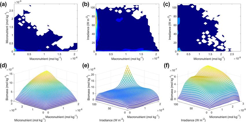
1944                                   C. Holder and A. Gnanadesikan: Understanding phytoplankton physiology using ML

Table 1. Details for each scenario that include the predictor variables, the target variable, the equations used to calculate biomass, the type
of source file used to acquire the values for the predictors, and a short description with important details about each scenario.

 Scenario     Predictors                     Target            Equations      Source file          Scenario description
                                                               used           description
 1            Macronutrient (mol kg−1 );     Biomass           1, 2, 3        Monthly output       (1) Nutrient distributions (predictors)
              micronutrient (mol kg−1 );     (mol kg−1 )                      from BLING              from BLING were run through
              irradiance (W m−2 )                                                                     Eqs. (1), (2), and (3) to calculate the
                                                                                                      biomass (target).
                                                                                                   (2) The true relationships were calcu-
                                                                                                      lated by using the range of the val-
                                                                                                      ues for the predictors and calculating
                                                                                                      the biomass based on Eqs. (1), (2),
                                                                                                      and (3).
 2            Macronutrient (mol kg−1 );     Biomass           1, 2, 3, 6     Daily output         (1) Hourly values for the predictors
              micronutrient (mol kg−1 );     (mol kg−1 )                      from BLING              were interpolated using the daily
              irradiance (W m−2 )                                                                     output of BLING.
                                                                                                     (1a) The macronutrient and micronu-
                                                                                                      trient hourly values were calculated
                                                                                                      using a standard interpolation be-
                                                                                                      tween the daily points.
                                                                                                     (1b) The irradiance hourly values
                                                                                                      were calculated from Eq. (6) using
                                                                                                      the value of the BLING daily input,
                                                                                                      hour of day, time of year, and
                                                                                                      location.
                                                                                                   (2) Hourly values of the predictors were
                                                                                                      fed to Eqs. (1), (2), and (3) to calcu-
                                                                                                      late hourly values for the biomass
                                                                                                      (target).
                                                                                                   (3) Daily-averaged values were calcu-
                                                                                                      lated by averaging 24 h for each lo-
                                                                                                      cation through 1 year.
                                                                                                   (4) Weekly-averaged values were calcu-
                                                                                                     lated by averaging 168 h blocks of
                                                                                                      time for each location through the
                                                                                                      year.
                                                                                                   (5) Monthly-averaged values were
                                                                                                      calculated by averaging the num-
                                                                                                      ber of hours in each month (days per
                                                                                                      month · 24) for each location through
                                                                                                      the year.
                                                                                                   (6) The true relationships were calcu-
                                                                                                      lated by using the range of the hourly
                                                                                                      values for the predictors and calcu-
                                                                                                      lating the biomass based on Eqs. (1),
                                                                                                      (2), and (3).
 3            Macronutrient (mol kg−1 );     Biomass           7, 8 (equa-    Monthly output       (1) Nutrient distributions from the
              micronutrient (mol kg−1 );     (mol kg−1 )       tions within   from BLING              BLING output were used as the pre-
              irradiance (W m−2 )                              BLING                                  dictors; biomass from the BLING
                                                               used to de-                            output itself was used as the target.
                                                               termine the
                                                               biomass)

Biogeosciences, 18, 1941–1970, 2021                                                           https://doi.org/10.5194/bg-18-1941-2021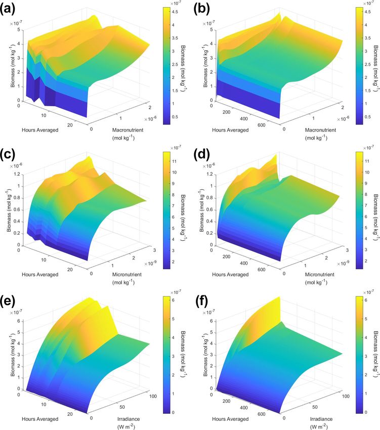
C. Holder and A. Gnanadesikan: Understanding phytoplankton physiology using ML                                              1945

   The final dataset consisted of three input/predictor vari-     25th to 75th percentiles are not considered outliers. Along
ables and one target term with a total of 77 328 observations.    those lines, we wanted to examine the conditions in a do-
The input variables given to each of three ML methods (mul-       main space that are likely to be found in actual observational
tiple linear regression (MLR), random forests (RF), and neu-      datasets, with the reasoning that if there was high uncertainty
ral network ensembles (NNE), described in more detail be-         in the ML predictions at these more moderate levels, there
low) were the concentrations (not the limitation terms) for       would be even higher uncertainty towards the extremes.
the micronutrient, macronutrient, and light. The target vari-         This method of sensitivity analysis contrasts with partial
able was the biomass we calculated from Eqs. (1)–(3). The         dependence plots (PDPs), which are commonly used in ML
same three ML methods were applied to all three scenarios.        visualization. PDPs show the marginal effect that predictors
   The dataset was then randomly split into training and test-    have on the outcome. They consider every combination of the
ing datasets, with 60 % of the observations going to the train-   values for a predictor of interest and all values of the other
ing dataset and the remainder going to the testing dataset.       predictors, essentially covering all combinations of the pre-
This provided a standard way to test the generalizability of      dictors. The predictions of a model are then averaged and
each ML method by presenting them with new observations           show the marginal effect of a predictor on the outcome –
from the test dataset and ensuring the models did not overfit     creating responses moderately comparable to averaged cross
the data. The input and output values for the training dataset    sections. Because of this averaged response, PDPs may hide
were used to train a model for each ML method. Once each          significant effects from subgroups within a dataset. A sen-
method was trained, we provided the trained models with the       sitivity analysis avoids this disadvantage by allowing sep-
input values of the testing dataset to acquire their respective   arate visualization of subgroup relationships. For example,
predictions. These predictions were then compared to the ac-      if macronutrient is the primary limiter over half of the do-
tual output values of the test dataset. To assess model perfor-   main, but not limiting at all over the other half, PDPs of
mance, we calculated the coefficient of determination (R 2 )      the biomass dependence on micronutrient will reflect this
and the root mean squared error (RMSE) between the ML             macronutrient limitation, while a sensitivity analysis at the
predictions and the actual output values for the training and     75th percentile of macronutrient will not.
testing datasets.                                                     Using the predictions produced from the sensitivity analy-
   Following this, a sensitivity analysis was performed on        ses, we also computed the half-saturation constants for each
the trained ML models. We allowed one predictor to vary           curve. A limitation of observational data is the frequency of
across its minimum–maximum range while holding the other          sampling, which limits the ability to estimate half-saturation
two input variables at specific percentile values. This was re-   coefficients without performing growth experiments in a lab.
peated for each predictor. This allowed us to isolate the im-     Calculating the half-saturation constants from the sensitivity
pact of each predictor on the biomass – creating cross sec-       analysis predictions allowed us to investigate if ML methods
tions of the dataset where only one variable changed at a         could provide a quantitative estimate from the raw observa-
time. For comparison, these values were also run through          tional data. The half-saturation constants were determined by
Eqs. (1)–(3) to calculate the true response of how the sim-       fitting a nonlinear regression model to each sensitivity anal-
ple phytoplankton model would behave. This allowed us to          ysis curve matching the form of a Michaelis–Menten curve
view which of the models most closely reproduced the un-          (Eq. 4):
derlying intrinsic relationships of the simple phytoplankton
                                                                        α1 N
model.                                                            B=          ,                                               (4)
   For our main sensitivity analyses, we chose to hold the             α2 + N
predictors that were not being varied at their respective 25th,   where B corresponds to the biomass predictions from the
50th, and 75th percentile values. We chose to use these par-      sensitivity analyses, N represents the nutrient concentrations
ticular percentile values for several reasons.                    from the sensitivity analyses, and α1 and α2 are the con-
   It allowed us to avoid the extreme percentiles (1st and        stants that are being estimated by the nonlinear regression
99th). As we approach these extremes, the uncertainty in the      model. The constant α2 was taken as the estimation of the
predictions grows quite rapidly because of the lack of train-     half-saturation coefficient for each sensitivity analysis curve.
ing samples within that domain space of the dataset. For ex-         Since colimitations can affect the calculation of half-
ample, there are no observations which satisfy the conditions     saturation coefficients, we also created interaction plots. This
of being in the 99th percentile of two variables simultane-       is useful because trying to calculate the half-saturation con-
ously. This extreme distance outside of the training domain       stant based on a nutrient curve that is experiencing limita-
generally leads to standard deviations in predictions that are    tion by another nutrient could cause the calculation to be un-
too large to provide a substantial level of certainty about the   derestimated. The interaction plots are a form of sensitivity
ML model’s predictions.                                           analysis where two predictor variables are varied across their
   Similar to the idea that we can avoid the extremes, we also    minimum–maximum range rather than one. This produces a
chose these values as they are quite typical values for the       mesh of predictor pairs covering the range of possible combi-
edges of box plots. Generally, values within the range of the     nations of two predictors. With these interaction plots, it was

https://doi.org/10.5194/bg-18-1941-2021                                                  Biogeosciences, 18, 1941–1970, 2021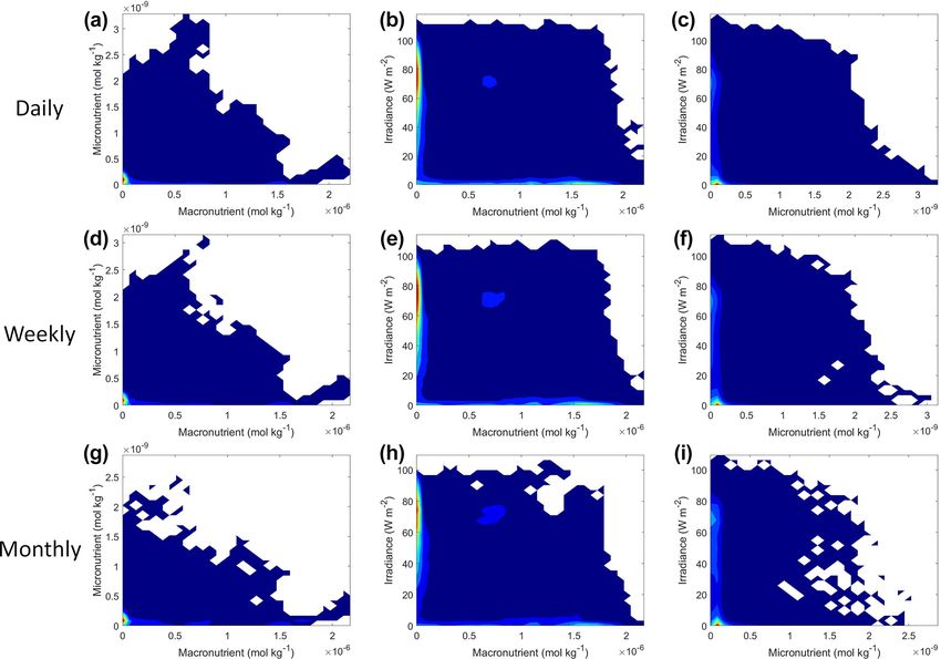
1946                                  C. Holder and A. Gnanadesikan: Understanding phytoplankton physiology using ML

possible to visualize the interaction of two variables and their     the only predictor variable that varied hourly. These hourly
combined effect on the target variable. For each pair of pre-        interpolated values were then used to calculate an hourly
dictors that were varying, we set the other predictor that was       biomass from Eqs. (1)–(3). Note that we are not claiming
not varying to its 50th percentile (median) value. As with the       real-world biomass would be zero at night but assume that
sensitivity analysis for single predictors, these predictor val-     on a long enough timescale, it should approach the average
ues were run through Eqs. (1)–(3) so a comparison could be           of the hourly biomass.
made as to which method most closely reproduced the true                To simulate apparent relationships, we smoothed the
variable interactions.                                               hourly values for both biomass and the input variables
                                                                     into daily, weekly, and monthly averages for each latitude–
2.2    Scenario 2: distantly related intrinsic and apparent          longitude point. To reiterate, the intrinsic and apparent rela-
       relationships on different timescales                         tionships in Scenario 2 differed in timescales but not in spa-
                                                                     tial scales. Each dataset was then analyzed following steps
In Scenario 1, the intrinsic relationships between environ-          similar to those outlined in Scenario 1; constructing train-
mental conditions and growth rate and apparent relationships         ing and testing datasets, using the same variables as inputs to
between environmental conditions and biomass differed only           predict the output (biomass), and using the same ML meth-
by a scale factor and operated at the same timescale. In real-       ods. To assess each method’s performance, we calculated the
ity, input variables (such as light) vary on hourly timescales       R 2 value and the RMSE between the predictions and ob-
so that growth rates vary on similar timescales. Biomass re-         servations for the training and testing datasets. We also per-
flects the average of this growth rate over many hours to days,      formed a sensitivity analysis, calculated half-saturation con-
while satellite observations and ESM model output are often          stants, and created interaction plots similar to those described
only available on monthly-averaged timescales. So the real-          above.
ity is that, even if a system is controlled by intrinsic relation-
ships, the apparent relationships gained from climatological         2.3    Scenario 3: BLING biogeochemical model
variables on long timescales will not reproduce these intrin-
sic relationships since the average light (irradiance) limita-       As a demonstration of their capabilities, the ML methods
tion is not equal to the limitation given the averaged light         were also applied directly to monthly-averaged output from
value (Eq. 5).                                                       the BLING model itself using the same predictors in scenar-
                                                               ios 1 and 2 but using the biomass calculated from the ac-
                − KIrr               − KIrr
LIrr = 1 − e         Irr    6= 1 − e     Irr   ,               (5)   tual BLING model. As described in Galbraith et al. (2010),
                                                                     BLING is a biogeochemical model where biomass is diag-
where the overbar denotes a time average, and Irr stands for         nosed as a nonlinear function of the growth rate smoothed
irradiance (light). For Scenario 2, we wanted to investigate         in time. The growth rates, in turn, have the same functional
how such time averaging biased our estimation of the intrin-         form as in scenarios 1 and 2, namely (Eq. 7)
sic relationships from the apparent ones; i.e., how does the
                                                                                                           Nmicro          Nmacro

link between the intrinsic and apparent relationships change         µ = µ0 · exp (k · T ) · min                      ,
                                                                                                       Kmicro + Nmicro Kmacro + Nmacro
with different amounts of averaging over time?
                                                                                    Irr
   For the short-timescale intrinsic relationships, we took            × 1 − exp −         ,                                                 (7)
                                                                                   IrrK
daily inputs for the three predictor variables for 1 year from
the ESM2Mc model. We further reduced the timescale from              where the first exponential parameterizes temperature-
days to hours to introduce daily variability for the irradiance      dependent growth following Eppley (1972), Nmacro and
variable relative to the latitude, longitude, and time of year       Nmicro are the macronutrient and micronutrient concentra-
(Eq. 6):                                                             tions, Kmacro and Kmicro are the half-saturation coefficients
                                                                   for the macronutrient and micronutrient, Irr is the irradiance,
             12π Irrdaily       π (t − tSunrise )
IrrInt (t) =              sin                                        and Irrk is a scaling for light limitation. An important differ-
               TDay                  TDay                            ence (to which we will return later in the paper) is that the
when 0 < t < TDay ,                                           (6)    light limitation term is calculated using a variable Chl : C ra-
                                                                     tio following the theory of Geider et al. (1997). The variation
where IrrInt is the hourly interpolated value of irradiance,
                                                                     of the Chl : C ratio would correspond to a KIrr in scenarios 1
Irrdaily is the daily-mean value of irradiance, t is the hour
                                                                     and 2 which adjusts in response to both changes in irradi-
of the day being interpolated, tSunrise is the hour of sunrise,
                                                                     ance (if nutrient is low) or changes in nutrient (if irradiance
and TDay is the total length of the day. The resulting curve
                                                                     is high), as well as changes in temperature. Given the result-
preserves the day-to-day variation in the daily mean irra-
                                                                     ing growth rate µ the total biomass then asymptotes towards
diance due to clouds and allows a realistic variation over
                                                                     (Eq. 8)
the course of the day. The hourly values for the micronu-
                                                                             µ̃ µ̃3

trient and macronutrient were assigned using a standard in-
terpolation between each of the daily values. Thus, light was        B=        + 3 S∗ ,                                           (8)
                                                                             λ λ

Biogeosciences, 18, 1941–1970, 2021                                                        https://doi.org/10.5194/bg-18-1941-2021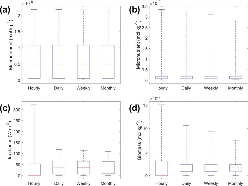
C. Holder and A. Gnanadesikan: Understanding phytoplankton physiology using ML                                                  1947

where λ = λ0 exp (k · T ) is a grazing rate, the tilde denotes an    marine ecological systems (Chase et al., 2007; Harding et al.,
average over a few days and S∗ is the biomass constant that          2015; Kruk et al., 2011).
we saw in the previous two scenarios. Note that because graz-
ing and growth have the same temperature dependence, the             2.4.1   Random forests
biomass then ends up depending on the nutrients and light in
a manner very similar to scenarios 1 and 2. Growth rates and         RFs are an ensemble ML method utilizing many decision
biomass are then combined to drive the uptake and water-             trees to turn “weak learners” into a single “strong learner”
column cycling of micronutrient and macronutrient within a           by averaging multiple outputs (Breiman, 2001). In general,
coarse-resolution version of the GFDL ESM2M fully cou-               RFs work by sampling (with replacement) about two-thirds
pled model (Galbraith et al., 2011), denoted as ESM2Mc.              of a dataset and constructing a decision tree. This process is
   As described in Galbraith et al. (2011) and Bahl et               known as bootstrap aggregation. At each split, the random
al. (2019), ESM2Mc produces relatively realistic spatial dis-        forest takes a random subset of the predictors and examines
tributions of nutrients, oxygen, and radiocarbon. Although           which variable can be used to split a given set of points into
simpler in its configuration relative to models such as TOPAZ        two maximally distinct groups. This use of random predic-
(Tracers of Ocean Phytoplankton with Allometric Zooplank-            tor subsets helps to ensure the model is not overfitting the
ton; Dunne et al., 2013), it has been demonstrated that in           data. The process of splitting the data is repeated until an op-
a higher-resolution physical model BLING produces simu-              timal tree is constructed or until the stopping criteria are met,
lations of mean nutrients, anthropogenic carbon uptake, and          such as a set number of observations in every branch (then
oceanic deoxygenation under global warming that are almost           called a leaf/final node). The process of constructing a tree is
identical to such complicated models (Galbraith et al., 2015).       then repeated a specified number of times, which results in
   We chose to use BLING for three main reasons. The first           a group (i.e., “forest”) of decision trees. Random forests can
is that we know it produces robust apparent relationships            also be used to construct regression trees in which a new set
between nutrients, light, and biomass by construction – al-          of observations traverse each decision tree with its associated
though these relationships can be relatively complicated –           predictor values, and the result from each tree is aggregated
particularly insofar as iron and light colimitation is involved      into an averaged value.
(Galbraith et al., 2010). As such, it represents a reasonable           Here, we used the same parameters for RF in the three sce-
challenge for a ML method to recover such nonlinear re-              narios to allow for a direct comparison between the scenar-
lationships. The second is that we know how these rela-              ios and to minimize the possible avenues for errors. Each RF
tionships are determined by the underlying intrinsic rela-           scenario was implemented using the TreeBagger function in
tionships between limiting factors and growth. Models with           MATLAB 2019b, where 500 decision trees were constructed
more complicated ecosystems (including explicit zooplank-            with each terminal node resulting in a minimum of five ob-
ton and grazing interactions between functional groups) may          servations per node (MATLAB, 2019). An optimization was
exhibit a more complicated time dependence that would con-           performed to decide the number of decision trees that mini-
fuse such a straightforward linkage between phytoplankton            mized the error while still having a relatively short runtime
growth limitation and biomass. The third is that despite its         of only several minutes. For additional details about the con-
simplicity, the model has relatively realistic annual mean           struction and training of the RFs, please see Appendix B.
distributions of surface nutrients, iron, and chlorophyll, and
under global warming, it simulates changes in oxygen and             2.4.2   Neural network ensembles
anthropogenic carbon uptake that are similar to much more
complicated ESMs (Galbraith et al., 2015).                           Neural networks (NNs) are another type of ML that has be-
                                                                     come increasingly popular in ecological applications (Flom-
2.4   ML algorithms                                                  baum et al., 2020; Franceschini et al., 2019; Guégan et
                                                                     al., 1998; Lek et al., 1996a, b; Mattei et al., 2018; Olden,
We chose to use random forests (RFs) and neural network en-          2000; Özesmi and Özesmi, 1999; Scardi, 1996, 2001; Scardi
sembles (NNEs) in this paper. Although other ML methods              and Harding, 1999). Scardi (1996) used NNs to model
exist, the list of possible choices is rather long. It was decided   phytoplankton primary production in the Chesapeake and
that the number of ML algorithms being compared would be             Delaware bays. Lek et al. (1996b) demonstrated the ability of
limited to RFs and NNEs, given their popularity in study-            NNs to explain trout abundance using several environmental
ing ecological systems. Additionally, we chose to compare            variables through the use of the “profiling” method, a type of
the performance of the ML techniques to the performance of           variable importance metric that averages the results of mul-
multiple linear regression (MLR), which allows us to quan-           tiple sensitivity analyses to acquire the importance of each
tify the importance of nonlinearity. It should be noted that         variable across its range of values.
we are not trying to suggest that MLR is always ineffective             Feed-forward NNs consist of nodes connected by weights
for studying ecological systems. MLR is a very useful and            and biases with one input layer, (usually) at least one hid-
informative approach for studying linear relationships within        den layer, and one output layer. The nodes of the input layer

https://doi.org/10.5194/bg-18-1941-2021                                                     Biogeosciences, 18, 1941–1970, 2021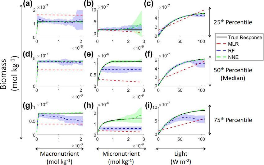
1948                                C. Holder and A. Gnanadesikan: Understanding phytoplankton physiology using ML

correspond to the input values of the predictor variables, and    no values are too close to the limits of the hyperbolic tan-
the hidden and output layer nodes each contain an activation      gent sigmoid activation function, which would significantly
function. Each node from one layer is connected to all other      increase the training time of each NN. Additionally, this nor-
nodes before and after it. The values from the input layer are    malization ensures that each predictor falls within a simi-
transformed by the weights and biases connecting the input        lar range, so more weight is not provided to variables with
layer to the hidden layer, put through the activation function    larger ranges. Although scaling is not necessary for RF and
of the hidden layer, modified by the weights and biases con-      MLR, the scalings used for the NNE were still applied to
necting the hidden layer to the output layer, and finally en-     each method for consistency. The results presented in this
tered into the final activation function of the output node.      paper were then transformed back to their original scales to
   The output (predictions) from this forward pass through        avoid confusion from scaling (Eq. 10).
the network is compared to the actual values, and the error is
calculated. This error is then used to update the weights with            maxU − minU
                                                                  VU =                (VS − minS ) + minU ,                    (10)
a backward pass through the network using backpropagation.                maxS − minS
The process is repeated a specified number of times or until
                                                                  where the letters represent the same values as in Eq. (9).
some optimal stopping criteria are met, such as error mini-
mization or validation checks where the error has increased
a specified number of times. For a more in-depth discussion       3     Results and discussion
of NNs, see Schmidhuber (2015).
   For this particular study, we use neural network ensem-        3.1    Scenario 1: closely related intrinsic and apparent
bles (NNEs), which are a collection of NNs (each of which                relationships on the same timescale
uses a subsample of the data) whose predictions are averaged
into a single prediction. It has been demonstrated that NNEs      In the first scenario, our main objective was to determine
can outperform single NNs and increase the performance of         if ML methods could extract intrinsic relationships when
a model by reducing the generalization error (Hansen and          given information on the apparent relationships and reason-
Salamon, 1990).                                                   able spatiotemporal distributions of colimitation when the in-
   To minimize the differences between scenarios, we used         trinsic and apparent relationships were operating on the same
the same framework for the NNs in each scenario. Each NN          timescale.
consisted of 3 input nodes (one for each of the predictor vari-      In Scenario 1, the RF and NNE both outperformed the
ables), 25 nodes in the hidden layer, and 1 output node. The      MLR as demonstrated by higher R 2 values and lower RMSE
activation function within the hidden nodes was a hyperbolic      (Table 2). The MLR captured just under half of the variance
tangent sigmoid function, and the activation function within      (R 2 = 0.44–0.45; Table 2), while the RF and NNE essen-
the output node used a linear function. The stopping crite-       tially captured all of it (R 2 > 0.99; Table 2). The decreased
ria for each NN was set as a validation check, such that the      performance of the MLR is not inherently surprising, given
training stopped when the error between the predictions and       the nonlinearity of the underlying model, but it does demon-
observations increased for six consecutive epochs. An op-         strate that the range of nutrients and light produced as inputs
timization was performed to decide the number of nodes in         by ESM2Mc are capable of producing a nonlinear response.
the hidden layer that minimized the error while maintaining a     Additionally, each method showed similar performances be-
short training time. A sensitivity analysis was also performed    tween the training and testing datasets, suggesting adequate
using different activation functions to ensure the choice of      capture of the model dynamics in both datasets.
activation function had minimal effect on the outcome. Fur-          From the spatial distributions and error plots of the true
thermore, another sensitivity analysis was performed to en-       response and the predictions from each method, it can be
sure additional hidden layers were not necessary. The details     observed that the RF and NNE showed the closest agree-
of the optimization and sensitivity analyses to determine the     ment with the true response (Fig. 1). The NNE showed the
NN parameters can be found in Appendix B.                         lowest error and closest agreement with the true response
   Each NNE consisted of 10 individual NNs, and each              (Fig. 1g), followed closely by the RF with slightly higher
NN was trained using the feedforwardnet function in MAT-          errors (Fig. 1f). Additionally, the RF and NNE were able to
LAB 2019b (MATLAB, 2019).                                         reproduce the biomass patterns in the equatorial Atlantic and
   Each variable was scaled between −1 and 1 based on its         Pacific, along with the low biomass concentrations at higher
respective maximum and minimum (Eq. 9).                           latitudes (Fig. 1a, c, d). Although MLR was able to repro-
                                                                  duce the general trend of the highest biomass in the low lati-
       maxS − minS
VS =               (VU − minU ) + minS ,                   (9)    tudes and low biomass in the high latitudes, it was not able to
       maxU − minU                                                predict higher biomass values (Fig. 1b), and it exhibited the
where V is the value of the variable being scaled, S stands       highest errors of the three methods (Fig. 1e).
for the scaled value (minimum is −1 and maximum is 1),               In addition to examining whether the different ML meth-
and U represents the unscaled value. This step ensures that       ods matched the correct response, we also interrogated these

Biogeosciences, 18, 1941–1970, 2021                                                  https://doi.org/10.5194/bg-18-1941-2021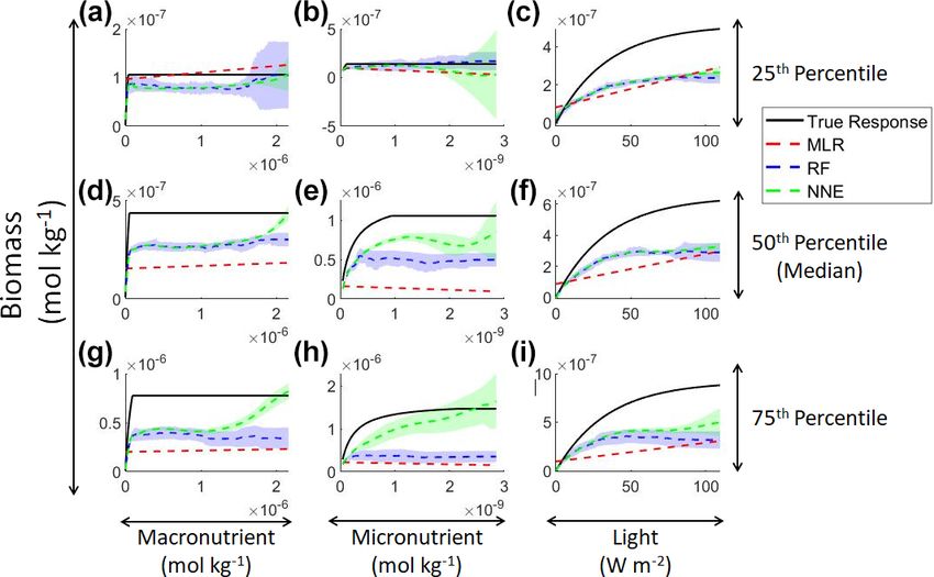
C. Holder and A. Gnanadesikan: Understanding phytoplankton physiology using ML 1949
Table 2. Performance metrics (coefficient of determination (R 2 ) and root mean squared error (RMSE)) for the training and testing datasets
of each scenario and the respective ML method (MLR – multiple linear regression; RF – random forest; NNE – neural network ensemble).
Scenario 2 had three time-averaged datasets (daily, weekly, and monthly). The target variable for all scenarios was phytoplankton biomass.
Training data Testing data
R2 RMSE R2 RMSE
Scenario 1 MLR 0.4528 1.32 × 10⁻⁷ 0.4471 1.33 × 10⁻⁷
RF 0.9989 6.46 × 10⁻⁹ 0.9977 9.15 × 10⁻⁹
NNE 0.9999 1.70 × 10⁻⁹ 0.9999 1.73 × 10⁻⁹
Scenario 2 Daily MLR 0.3160 8.75 × 10⁻⁸ 0.3104 8.82 × 10⁻⁸
RF 0.9841 1.35 × 10⁻⁸ 0.9684 1.90 × 10⁻⁸
NNE 0.9686 1.88 × 10⁻⁸ 0.9681 1.90 × 10⁻⁸
Weekly MLR 0.3054 8.35 × 10⁻⁸ 0.3059 8.31 × 10⁻⁸
RF 0.9835 1.30 × 10⁻⁸ 0.9687 1.78 × 10⁻⁸
NNE 0.9680 1.79 × 10⁻⁸ 0.9688 1.76 × 10⁻⁸
Monthly MLR 0.3022 8.07 × 10⁻⁸ 0.3125 8.01 × 10⁻⁸
RF 0.9859 1.16 × 10⁻⁸ 0.9729 1.60 × 10⁻⁸
NNE 0.9722 1.61 × 10⁻⁸ 0.9722 1.61 × 10⁻⁸
Scenario 3 MLR 0.0672 2.55 × 10⁻⁸ 0.0691 2.53 × 10⁻⁸
RF 0.9727 4.49 × 10⁻⁹ 0.9445 6.26 × 10⁻⁹
NNE 0.9417 6.38 × 10⁻⁹ 0.9386 6.50 × 10⁻⁹
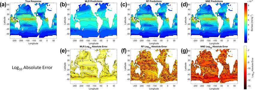
Figure 1. The contour plots in the top row show the yearly-averaged biomass of Scenario 1 for the true response (a) and the associated
predictions from MLR (b), RF (c), and NNE (d). The biomass was measured in units of mol kg−1 . The contour plots in the bottom row show
the log10 absolute error between the true response and the predictions from MLR (e), RF (f), and NNE (g).
methods to look at how different predictors contributed to lines) showed agreement with the true response of the model
the answer and whether these contributions matched the in- (black lines) in all circumstances, insofar as the true response
trinsic relationships between the predictors and biomass as was always within the standard deviation of the NNE predic-
we had put into the model (Fig. 2). The MLR (red dashed tions (Fig. 2).
lines) showed very little response to changes in macronu- The RF prediction of the response to a given predictor
trient (Fig. 2a, d, g), an unrealistic negative response to in- (blue dashed lines) showed agreement with the true response
creases in micronutrient (Fig. 2b, e, h), and a reasonable (al- when the other predictors were fixed at the lower percentiles
beit linear) match to the light response (Fig. 2c, f, i). By con- (Fig. 2a–c) but began deviating in the higher percentiles
trast, the response to any predictor for the NNE (green dashed (Fig. 2d–i). This was likely due to the range of the training
https://doi.org/10.5194/bg-18-1941-2021 Biogeosciences, 18, 1941–1970, 2021
1950                                   C. Holder and A. Gnanadesikan: Understanding phytoplankton physiology using ML

Figure 2. Sensitivity analysis for Scenario 1 showing the true and predicted relationships for each ML method. The columns correspond to
the predictors, and the rows correspond to the percentile value at which the other predictors were set (e.g., panel a varies the macronutrient
across its minimum–maximum range, while the micronutrient and light are held at their 25th percentile values, respectively). The black
line shows the true intrinsic relationship calculated from Eqs. (1)–(3). The dashed lines show the predicted apparent relationships for each
method (MLR – red; RF – blue; NNE – green). The RF and NNE predicted relationships are the average of the individual predictions for each
method. The colored regions around the RF and NNE dashed lines show 1 standard deviation in the predictions (e.g., 1 standard deviation in
the 10 individual NN predictions of the NNE).

dataset and how RFs acquire their predictions. When pre-                 Liebig’s law of the minimum applies to the two nutrient lim-
sented with predictor information, RFs rely on the informa-              itations. When the micronutrient is low, it prevents the entire
tion contained within their training data. If they are presented         Michaelis–Menten curve for the macronutrient from being
with predictor information that goes outside the range of the            seen.
data space of the training set, RFs will provide a prediction               Although the NNEs captured the true intrinsic relation-
based within the range of the training set. When perform-                ships, we could not interpret these curves without remem-
ing the sensitivity analysis, the values of the predictors in            bering that multiple limitations affect biomass. For example,
the higher percentiles were outside the range of the training            when we computed an estimated half-saturation for the nu-
dataset. For example, RF deviates from the true response as              trient curves in the top row of Fig. 2, we calculated values for
the concentration of the macronutrient increases – actually              KN that were far lower than the actual ones specified in the
decreasing as nutrient increases despite the fact that such a            model (Table 3). The estimated half-saturation when other
result is not programmed into the underlying model (Fig. 2g).            predictors were held at their 25th percentile for the micro-
Although there may be observations in the training dataset               and macronutrient was underestimated by one and two orders
where the light and micronutrient are at their 75th percentile           of magnitude, respectively. When higher percentiles were
values when the macronutrient is low, there likely are not               used (Table 4), the estimated half-saturation was overesti-
any observations where high levels of the macronutrient, mi-             mated for some predictors and underestimated for others.
cronutrient, and light are co-occurring. Without any observa-            At the 99th percentile, the macronutrient half-saturation was
tions meeting that criteria, the RF provided the highest pre-            underestimated by 49 %, and micronutrient and light were
diction it could based on the training information.                      overestimated by 77 % and 36 %, respectively (Table 4). It
   In contrast to the RF’s inability to extrapolate outside the          is possible that, even at the higher percentiles, micronutrient
training range, the NNE showed its capability to make pre-               was still exerting some limitation on the macronutrient curve,
dictions on observations on which it was not trained (Fig. 2).           which would explain why the estimate for the macronutrient
Note, however, that while we have programmed Michaelis–                  half-saturation was underestimated. However, this does not
Menten intrinsic dependencies for individual limitations into            explain why the estimations for the micronutrient and light
our model, we did not get Michaelis–Menten type curves                   half-saturations were overestimated by so much. Although
back for macro- and micronutrients when the other variables              the ability to calculate half-saturation coefficients from the
were set at low percentiles (Fig. 2a–c). The reason is that              sensitivity analysis curves seemed to be a way to quantify

Biogeosciences, 18, 1941–1970, 2021                                                           https://doi.org/10.5194/bg-18-1941-2021
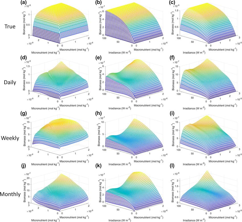
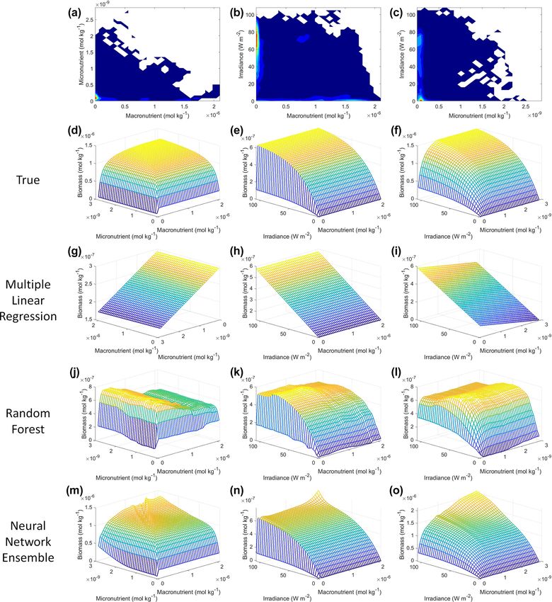
C. Holder and A. Gnanadesikan: Understanding phytoplankton physiology using ML                                              1951

the accuracy of the ML predictions, colimitations lead to          a pattern of Liebig minimization. It was interesting that
high uncertainties in the estimates. While mathematically          the macronutrient–irradiance interaction (Fig. 3n) almost ap-
obvious, this result has implications for attempts to extract      peared to display a pattern of no colimitation (Saito et al.,
(and interpret) KN from observational datasets, such that one      2008, their Fig. 2A), but this stark increase in the biomass
would expect colimitation to produce a systematic underesti-       past low concentrations of the macronutrient can be partially
mation of KN .                                                     explained by the contour plot of observations (Fig. 3b; please
   In an effort to visualize the colimitations and to investi-     see Fig. C1 in Appendix C for individual box plots of the
gate the extent to which any of the methods could reproduce        predictor and target variables). The majority of observations
these interactions, we examined the interaction plots (Fig. 3).    where macronutrient concentrations were low had a corre-
MLR expectedly predicted linear relationships in which             spondingly high value for irradiance. Additionally, when the
higher-concentration pairs of irradiance–macronutrient and         macronutrient passed a certain concentration (which hap-
irradiance–micronutrient lead to higher biomass (Fig. 3h, i),      pened to be very low in these conditions), the micronutri-
but it incorrectly predicted the interaction between the micro-    ent became the limiting nutrient, such that light was the only
and macronutrient such that decreasing concentrations of           variable that then affected the biomass (data not shown).
macronutrient lead to higher biomass (Fig. 3g). Note that the         With respect to our main objective for Scenario 1, it was
x and y axes in Fig. 3g were switched relative to the other        evident that only the NNE was able to extract the intrinsic
subplot axes, which was necessary to visualize the interac-        relationships from information on the apparent relationships.
tion. RF incorrectly predicted the highest concentrations of       This was due in large part to its capability of extrapolating
biomass at moderate levels of the micro- and macronutrient         outside the range of the training dataset, whereas RFs were
in their interactions with irradiance (Fig. 3k, l). RF again in-   constrained by training data, and MLR was limited by its in-
correctly predicted the greatest biomass in the micronutrient–     herent linearity and simplicity. Furthermore, the attempts to
macronutrient interaction occurring at low levels of micronu-      quantify the half-saturation coefficients from the sensitivity
trient across most levels of macronutrient (Fig. 3j). The NNE      analysis curves proved unreliable because of nutrient colim-
was the only method that was able to reproduce the interac-        itations. However, we were able to use interaction plots to
tions of the model (Fig. 3d–f, m–o). Although the NNE over-        qualitatively describe the type of colimitation occurring be-
estimated the biomass prediction when concentrations were          tween each pair of predictors and support the result from the
high for both predictors in the irradiance–micronutrient and       single predictor sensitivity analyses that micronutrient was
irradiance–macronutrient interactions (Fig. 3e, f, n, o), these    most limiting in many situations.
were also the areas of the data space without any observa-
tions to constrain the NNE (Fig. 3b, c). Similar to the sensi-     3.2   Scenario 2: distantly related intrinsic and apparent
tivity analyses for single predictors, the NNE was capable of            relationships on different timescales
extrapolating outside the range of the training dataset while
RF was not.                                                        In Scenario 1, the intrinsic and apparent relationships were
   The NNE interaction plots (Fig. 3m–o) bear resemblance          simply related by a scaling factor. In practice, the relation-
to the colimitation plots seen in Fig. 2 of Saito et al. (2008)    ships are more difficult to connect to each other. For the sec-
and allowed for a qualitative comparison of the type of col-       ond scenario, both the output biomass and predictors (light,
imitation that two predictors have on the target variable.         macronutrient, and micronutrient) were averaged over daily,
For example, the micronutrient–macronutrient interaction in        weekly, and monthly timescales. Our main objective was to
Fig. 3m shows the same type of response as would be                investigate how the link between intrinsic and apparent rela-
expected in Liebig minimization (Saito et al., 2008, their         tionships changed when using climatologically averaged data
Fig. 2C). This result is what we would expect given that the       – as is generally the case for observational studies.
equations for Scenario 1 (Eqs. 1–3) were Liebig minimiza-             As in Scenario 1, the RF and NNE outperformed the MLR
tion by construction between the macro- and micronutrient.         based on the performance metrics for the daily, weekly, and
Additionally, Liebig minimization can be seen in the pattern       monthly time-averaged scenarios (Table 2), with linear mod-
displayed in the interaction plot of the true expected response    els only able to explain about 30 % of the variance. The
(Fig. 3d).                                                         comparable performances between the training and testing
   The interactions of macronutrient–irradiance (Fig. 3n) and      datasets suggested a sufficient sampling of the data for each
micronutrient–irradiance (Fig. 3o) mirrored the colimitation       method to capture the dynamics of the underlying model.
pattern of independent multiplicative nutrients (Saito et al.,        Examining the monthly apparent relationships found for
2008, their Fig. 2B) where neither predictor was limiting,         each method and comparing them to the true intrinsic rela-
and the effects of the two predictors have a multiplicative        tionships showed that none of the methods were able to re-
effect on the target variable. This was again consistent with      produce the true intrinsic relationships – in general system-
the equations that govern Scenario 1 (Eqs. 1–3). In Eq. (1),       atically underestimating biomass at high levels of light and
the irradiance limitation was only multiplied by the lesser        nutrient (Fig. 4). The one exception was the 25th percentile
limitation of the macro- and micronutrient and did not show        plot of the micronutrient (Fig. 4b). The underestimation was

https://doi.org/10.5194/bg-18-1941-2021                                                   Biogeosciences, 18, 1941–1970, 2021
1952                                    C. Holder and A. Gnanadesikan: Understanding phytoplankton physiology using ML

Table 3. The true value and estimated half-saturation coefficients for each scenario and predictor (macronutrient, micronutrient, and light)
based on the 25th, 50th, and 75th percentiles. The percentiles correspond to the values at which the other predictors were set (e.g., for the
25th percentile macronutrient value, the macronutrient varied across its minimum–maximum range, while micronutrient and light were set at
their respective 25th percentile values). The coefficients were estimated using a nonlinear regression function to fit a curve to the predictions
in the sensitivity analyses of the form in Eq. (4), where α2 was the estimate for each half-saturation coefficient.

                                                                                            NNE
                                                                         Macronutrient       Micronutrient     Light
                           True value                                      1.00 × 10⁻⁷       2.00 × 10⁻¹⁰      34.30
                           Scenario 1                 25th percentile      6.27 × 10⁻⁹        1.29 × 10⁻⁹      38.91
                                                      50th percentile      1.04 × 10⁻⁸       1.44 × 10⁻¹⁰      38.26
                                                      75th percentile      1.88 × 10⁻⁸       2.86 × 10⁻¹⁰      40.09
                           Scenario 2     Daily       25th percentile      9.87 × 10⁻⁹     −9.85 × 10⁻¹¹       22.04
                                                      50th percentile      3.22 × 10⁻⁸       1.88 × 10⁻¹⁰      23.20
                                                      75th percentile      4.89 × 10⁻⁸       3.51 × 10⁻¹⁰      20.09
                                          Weekly      25th percentile      1.08 × 10⁻⁸     −6.48 × 10⁻¹⁰       26.18
                                                      50th percentile      3.78 × 10⁻⁸       1.92 × 10⁻¹⁰      25.50
                                                      75th percentile      6.36 × 10⁻⁸        1.11 × 10⁻⁹      18.49
                                          Monthly     25th percentile      7.64 × 10⁻⁹     −6.90 × 10⁻¹⁰       23.13
                                                      50th percentile      3.26 × 10⁻⁸       1.63 × 10⁻¹⁰      19.37
                                                      75th percentile      1.38 × 10⁻⁷        1.04 × 10⁻⁹      21.89
                           Scenario 3                 25th percentile      3.50 × 10⁻⁸          6.84 × 10²      1.85
                                                      50th percentile      8.89 × 10⁻⁸       6.94 × 10⁻¹⁰       5.80
                                                      75th percentile      1.64 × 10⁻⁷        2.41 × 10⁻⁹       7.78

consistent across the different timescales, and the sensitiv-              environment to intrinsic relationships from the laboratory, it
ity analysis showed little difference in the predicted rela-               is essential to take into account which timescales of variabil-
tionships between the daily, weekly, and monthly-averaged                  ity that averaging has removed. Insofar as most variability is
timescales for the NNEs (Fig. 5). Because the NNEs showed                  at hourly timescales, daily-, weekly-, and monthly-averaged
the closest approximations to the correct shape and magni-                 data will produce very similar apparent relationships (Fig. 5).
tude of the curves compared to RF and MLR (Fig. 4), the                    But if there was a strong week-to-week variability in some
remaining analysis of Scenario 2 is mainly focused on NNEs.                predictor, this may not be the case.
   The underestimation was not entirely unexpected. The av-                   To understand how the apparent relationships were chang-
eraging of the hourly values into daily, weekly, and monthly               ing across different timescales, we averaged the hourly
timescales quickly leads to a loss of variability (Fig. 6), es-            dataset over a range of hourly time spans. Specifically, we
pecially for light (Fig. 6c). A large portion of the variabil-             averaged over the timescales of 1 (original hourly set), 2,
ity was lost in the irradiance variable going from hourly to               3, 4, 6, 8, 12, 24, 48, 72, 168 (weekly), and 720 (monthly)
daily (Fig. 6c). The loss of variability meant that the light              hours. This new set of averaged timescales was then used
limitation computed from the averaged light was systemat-                  to train NNEs with one NNE corresponding to each aver-
ically higher than the averaged light limitation. To match                 aged timescale. We then performed sensitivity analyses on
the observed biomass, the asymptotic biomass at high light                 each of the trained NNEs to see the apparent relationships for
would have to be systematically lower (see Appendix A for                  each averaged timescale and set the percentile vales for the
the mathematical proof). Differences were much smaller for                 other variables at their 50th percentile (median). For more
macronutrient and micronutrient as they varied much less                   details about this method, please see Appendix D. To visu-
over the course of a month in our dataset. Our results em-                 alize all the timescales at once, we plotted them on surface
phasize that when comparing apparent relationships in the                  plots (Fig. 7). The greatest changes in the apparent relation-

Biogeosciences, 18, 1941–1970, 2021                                                             https://doi.org/10.5194/bg-18-1941-2021
You can also read