The tipping points and early warning indicators for Pine Island Glacier, West Antarctica
←
→
Page content transcription
If your browser does not render page correctly, please read the page content below
The Cryosphere, 15, 1501–1516, 2021
https://doi.org/10.5194/tc-15-1501-2021
© Author(s) 2021. This work is distributed under
the Creative Commons Attribution 4.0 License.

The tipping points and early warning indicators for Pine Island
Glacier, West Antarctica
Sebastian H. R. Rosier1 , Ronja Reese2 , Jonathan F. Donges2,3 , Jan De Rydt1 , G. Hilmar Gudmundsson1 , and
Ricarda Winkelmann2,4
1 Department    of Geography and Environmental Sciences, Northumbria University, Newcastle, UK
2 Earth  System Analysis, Potsdam Institute for Climate Impact Research (PIK), Member of the Leibniz Association,
P.O. Box 60 12 03, 14412 Potsdam, Germany
3 Stockholm Resilience Centre, Stockholm University, Kräftriket 2B, 10691 Stockholm, Sweden
4 Institute of Physics and Astronomy, University of Potsdam, Karl-Liebknecht-Str. 24–25, 14476 Potsdam, Germany

Correspondence: Sebastian H. R. Rosier (sebastian.rosier@northumbria.ac.uk)

Received: 30 June 2020 – Discussion started: 4 August 2020
Revised: 21 January 2021 – Accepted: 31 January 2021 – Published: 25 March 2021

Abstract. Mass loss from the Antarctic Ice Sheet is the main         1   Introduction
source of uncertainty in projections of future sea-level rise,
with important implications for coastal regions worldwide.
Central to ongoing and future changes is the marine ice              The West Antarctic Ice Sheet (WAIS) is regarded as a tip-
sheet instability: once a critical threshold, or tipping point, is   ping element in the Earth’s climate system, defined as a ma-
crossed, ice internal dynamics can drive a self-sustaining re-       jor component of the Earth system susceptible to tipping-
treat committing a glacier to irreversible, rapid and substan-       point behaviour (Lenton et al., 2008). Its collapse, potentially
tial ice loss. This process might have already been triggered        driven by the marine ice sheet instability (MISI; Feldmann
in the Amundsen Sea region, where Pine Island and Thwaites           and Levermann, 2015), would result in over 3 m of sea-level
glaciers dominate the current mass loss from Antarctica, but         rise (Fretwell et al., 2013). Key to MISI are the conditions at
modelling and observational techniques have not been able            the grounding line – the transition across which grounded ice
to establish this rigorously, leading to divergent views on the      begins to float on the ocean forming ice shelves. In a steady
future mass loss of the West Antarctic Ice Sheet. Here, we           state, ice flux across the grounding line balances the sur-
aim at closing this knowledge gap by conducting a systematic         face accumulation upstream. If grounding-line retreat causes
investigation of the stability regime of Pine Island Glacier.        grounding-line flux to increase and this is not balanced by
To this end we show that early warning indicators in model           a corresponding increase in accumulation, the net mass bal-
simulations robustly detect the onset of the marine ice sheet        ance is negative and retreat will continue (Weertman, 1974;
instability. We are thereby able to identify three distinct tip-     Schoof, 2007). Conversely, grounding-line advance leading
ping points in response to increases in ocean-induced melt.          to an increase in accumulation greater than the change in
The third and final event, triggered by an ocean warming of          flux will lead to a continued advance. In this regime, a small
approximately 1.2 ◦ C from the steady-state model configura-         perturbation in the system can result in the system crossing
tion, leads to a retreat of the entire glacier that could initiate   a tipping point, beyond which a positive feedback propels
a collapse of the West Antarctic Ice Sheet.                          the system to a contrasting state (Fig. 1c). A complex range
                                                                     of factors can either cause or suppress MISI (Haseloff and
                                                                     Sergienko, 2018; Pegler, 2018; O’Leary et al., 2013; Gomez
                                                                     et al., 2010; Robel et al., 2016), and the difficulties in pre-
                                                                     dicting this behaviour are a major source of uncertainty for
                                                                     future sea-level-rise projections (Church et al., 2013; Bamber
                                                                     et al., 2019; Oppenheimer et al., 2019; Robel et al., 2019).

Published by Copernicus Publications on behalf of the European Geosciences Union.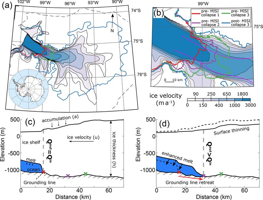
1502                                                                       S. H. R. Rosier et al.: Tipping points of Pine Island Glacier

                                                                             ing whether a tipping point has been crossed is that currently
                                                                             this necessitates time-consuming steady-state simulations to
                                                                             calculate the hysteresis behaviour of an identified period of
                                                                             retreat (e.g. Garbe et al., 2020). An alternative methodology
                                                                             that can be applied directly to transient simulations as a post-
                                                                             processing step would therefore be useful to the ice sheet
                                                                             modelling community. Such tools based on early warning in-
                                                                             dicators are presented in this paper.
                                                                                The tipping behaviour of MISI is an example of a saddle-
                                                                             node (or fold) bifurcation in which three equilibria exist: an
                                                                             upper and lower stable branch and a middle unstable branch
                                                                             (Fig. 1c; Schoof, 2012). Starting on the upper stable branch,
                                                                             perturbing the system beyond a tipping point (x1 in Fig. 1c)
                                                                             will induce a qualitative shift to the lower and contrasting sta-
                                                                             ble state. Importantly (and in contrast to a system such as that
                                                                             shown in Fig. 1a and b), in order to restore conditions to the
                                                                             state prior to a collapse it is not sufficient to simply reverse
                                                                             the forcing to its previous value. Instead, the forcing must be
                                                                             taken back further (to point x2 ), which in some cases may be
                                                                             far beyond the parameter range that triggered the initial col-
                                                                             lapse. This type of behaviour is known as hysteresis. A large
Figure 1. Possible range of behaviours for a system state (e.g. ice          change in response to a small forcing is not necessarily in-
flux) in response to perturbations in a control parameter (e.g. ocean        dicative of hysteresis, as shown in Fig. 1b. Tipping points are
temperature). A system can (a) respond to a perturbation in a lin-           crossed in both Fig. 1c and Fig. 1d, and both cases are often
ear way that is directly recoverable with a reversal of the forcing;         referred to as irreversible, although the two are distinct in that
(b) have a large response to a small perturbation that is still directly     only Fig. 1d is irreversible for any change in the tested range
recoverable; (c) have a large response to a small perturbation that          of the control parameter. Hereafter we will refer to the former
is irreversible (hysteresis behaviour); and (d) have a large response        as irreversible, in line with previous studies, and the latter as
that is irreversible for any change in the tested range of the control       permanently irreversible, to differentiate the two. Diagnos-
parameter, a behaviour we refer to as permanently irreversible (no
                                                                             ing whether a tipping point has been crossed without some
recovery possible even if forcing is reversed well below the initial
level). Tipping points are crossed only in panels (c) and (d) and are
                                                                             prior knowledge of the system is not generally possible with-
indicated by x1 , x2 and x3 . Panel (c) also shows a transient response      out reversing the forcing to see if hysteresis has occurred. An
in which the system state lags behind changes in the control param-          alternative approach to identify tipping points is based on a
eter as is the case for ice sheets and thus crosses the irreversible         process known as critical slowing down, which is known to
system state at a later point, xt .                                          precede saddle-node bifurcations of this type (Wissel, 1984;
                                                                             van Nes and Scheffer, 2007; Dakos et al., 2008; Scheffer et
                                                                             al., 2009). Critical slowing down is a general feature of non-
   One area of particular concern is the Amundsen Sea re-                    linear systems and refers to an increase in the time a system
gion. Pine Island (PIG) and Thwaites glaciers, the two largest               takes to recover from perturbations as a tipping point is ap-
glaciers in the area, are believed to be particularly vulnerable             proached (Wissel, 1984). We will explore both hysteresis and
to MISI (Favier et al., 2014; Rignot et al., 2014). Palaeo-                  critical slowing down as indicators of tipping points in our
records and observational records of PIG show a history of                   model simulations.
retreat, driven by both natural and anthropogenic variability                   In Sect. 2, we explain critical slowing down and early
in ocean forcing (Jenkins et al., 2018; Holland et al., 2019).               warning indicators in the context of MISI. We then map out
One possible MISI-driven retreat might have happened when                    the stability regime of PIG using numerical model simula-
PIG unpinned from a submarine ridge in the 1940s (Jenkins                    tions. We force the model with a slowly increasing ocean
et al., 2010; Smith et al., 2016). Recent modelling studies                  melt rate and identify three periods of rapid retreat with
indicate that a larger-scale MISI event may now be under-                    the methodology explained in Sect. 3.1. Using statistical
way for both Pine Island and Thwaites glaciers that would                    tools from dynamical systems theory we find critical slow-
lead to substantial and sustained mass loss throughout the                   ing down preceding each of these retreat events and go on to
coming centuries (Favier et al., 2014; Jenkins et al., 2016;                 demonstrate that these are indeed tipping points in Sect. 4.
Joughin et al., 2010). Being able to identify a MISI-driven                  This is confirmed by analysing the hysteresis behaviour of
retreat and differentiate this from a retreat where a tipping                the glacier, showing the existence of unstable grounding-line
point has not been crossed is vital information for projections              positions. To our knowledge, this is the first time that the
of future sea-level rise. One of the major hurdles in determin-              stability regime of PIG has been investigated in this detail

The Cryosphere, 15, 1501–1516, 2021                                                              https://doi.org/10.5194/tc-15-1501-2021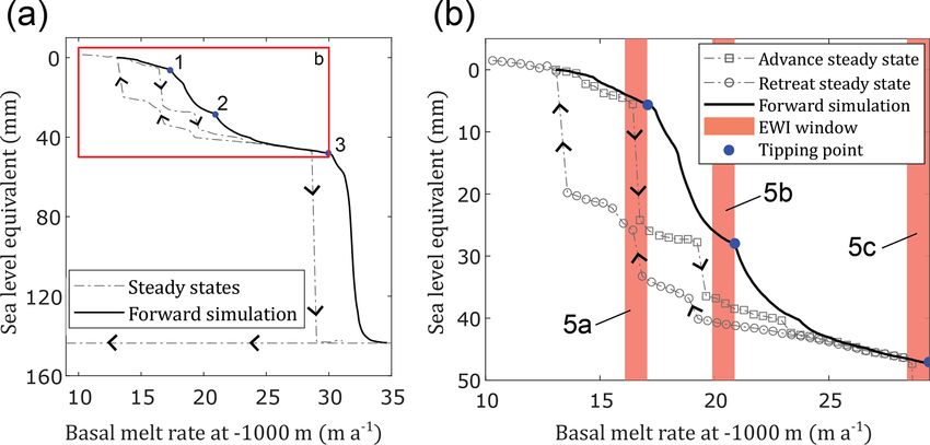
S. H. R. Rosier et al.: Tipping points of Pine Island Glacier                                                                  1503

and the first time that tipping-point indicators have been ap-      setup, we determine the change in recovery time before a tip-
plied to ice sheet model simulations. Our results reveal the        ping point directly through multiple stepwise perturbations
existence of multiple tipping points leading to the collapse        of the control parameter (Appendix A). Our setup closely re-
of PIG, rather than one single event, that when crossed could       sembles the MISMIP experiments (Pattyn et al., 2012), and
easily be misidentified as simply periods of rapid retreat, with    indeed hints of critical slowing down can be identified in
the irreversible and the self-sustained aspect of the retreat be-   that paper (Fig. 2 in Pattyn et al., 2012). The results in Ap-
ing missed.                                                         pendix A show that critical slowing down is easily identified
                                                                    preceding both MISI-driven advance and retreat bifurcations.
                                                                    This demonstrates that there is at least the potential that crit-
2     Critical slowing down and early warning indicators            ical slowing down could be found in a less simplified mod-
                                                                    elling framework. This is not clear a priori, and, for exam-
As certain classes of complex systems approach a tipping            ple, adding noise to the bed topography reduces the ability to
point, they show early warning signals (i.e. specific changes       identify early warning, as detailed in the Appendix. Identify-
in system behaviour as detailed below) which can allow us           ing critical slowing down in this stepwise perturbation man-
to anticipate or even predict the onset of a tipping event          ner is appealing because it directly extracts the change in re-
by means of statistical tools called early warning indica-          sponse time that we are searching for; however it is not prac-
tors (EWIs; Wissel, 1984). Early warning signals have been          tical for a realistic model forcing which would not normally
found to precede, for example, collapse of the thermoha-            take the form of a step function. A more general approach,
line circulation (Held and Kleinen, 2014; Lenton, 2011), on-        which we adopt for our simulation of PIG, is to use EWIs to
set of epileptic seizures (Litt et al., 2001; McSharry and          analyse the recovery time of the system as it is forced with
Tarassenko, 2003), crashes in financial markets (May et             natural variability.
al., 2008; Diks et al., 2018), onset of glacial terminations
(Lenton, 2011) and wildlife population collapses (Scheffer et       2.2   Early warning indicators
al., 2001). Although most commonly used to detect the onset
of saddle-node bifurcations, of which MISI is an example,           As the field of EWIs has expanded, more methods have been
they are not strictly limited to bifurcations of this type and      developed for extracting critical-slowing-down information
have, for example, also been successfully used to indicate          from model results and observational records. These meth-
the onset of Hopf bifurcations (Chisholm and Filotas, 2009).        ods seek to approximate the system recovery time from some
                                                                    measure of the system state. The challenge is that, for most
2.1    Critical slowing down preceding the marine ice               real-world applications, natural forcing does not take the
       sheet instability                                            form of a step function and the system is continuously per-
                                                                    turbed and so cannot return to a true steady state. However,
Critical slowing down is one example of an early warning            if the recovery time of a system is indeed increasing, the re-
signal that has been used in the past for both model out-           sponse to a continual stochastic forcing could be detected
put and observational records such as palaeoclimate data,           as a tendency for each measurement of the system state to
with the aim of detecting an approaching bifurcation (Held          become increasingly similar to the previous measurement,
and Kleinen, 2004; Livina and Lenton, 2007; Dakos et al.,           sometimes referred to as an increase in “memory” of small
2008; Lenton et al., 2009, 2012b). Critical slowing down is         perturbations. This is shown conceptually and with examples
so called because, as a non-linear system is gradually forced       extracted from our PIG model in Fig. 2. One common way
towards a bifurcation, that system will become more “slug-          to measure this effect is by sampling the data at discrete time
gish” in its response to perturbations (see middle panel of         intervals and calculating the lag-1 auto-correlation, i.e. the
Fig. 2). This can be shown mathematically, because the dom-         correlation between values that are one time interval apart
inant eigenvalue of the system tends to zero as a bifurcation       (examples given in Fig. 2). This measure, which we refer to
point is approached (Wissel, 1984) or, equivalently, the re-        hereafter as the ACF indicator, should increase as a tipping
covery time (i.e. the time it takes for a system to return to a     point is approached (Dakos et al., 2008; Ives, 1995). Since re-
steady state after small perturbations) tends to infinity. The      covery time tends to infinity as the bifurcation is approached,
response time of a glacier to external forcing has also been        successive system states should become more and more sim-
shown analytically to increase as a MISI bifurcation is ap-         ilar and the ACF indicator should tend to 1. This threshold
proached (Robel et al., 2018). While critical slowing down is       of an indicator, corresponding to the point when a tipping
a general characteristic behaviour of the dynamics underly-         point would be crossed as predicted by theory, is referred
ing MISI, the question remains whether it can be reliably de-       to hereafter as the critical value. An alternative measure that
tected in the context of a complex glacier where many other         also seeks to identify changes in recovery time is to use the
processes are at play.                                              detrended fluctuation analysis algorithm (Livina and Lenton,
   As a first step to addressing this question, we model MISI       2007; Lenton et al., 2012a, b). This first calculates the mean-
in an idealised flow line setup of a marine ice sheet. In this      centred cumulative sum of the time series, splits the result

https://doi.org/10.5194/tc-15-1501-2021                                                   The Cryosphere, 15, 1501–1516, 2021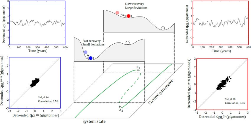
1504                                                                     S. H. R. Rosier et al.: Tipping points of Pine Island Glacier

Figure 2. Critical slowing down can serve as an indicator that the system is approaching a tipping point. This can be understood conceptually
using the common “ball on a slope” analogy (middle panel), where the ball represents the system state and minima are stable equilibrium
states. Two example cases are superimposed onto their corresponding positions in the hysteresis plot of MISI shown by the green line and
equivalent to Fig. 1c. The processed model results demonstrate how critical slowing down manifests itself, as shown in the blue and red
panels at the sides. If the system is far from a tipping point (blue case), the system state (which is in this study the grounding-line flux qGL ,
upper left panel) recovers quickly from perturbations in the control parameter (which is here the basal melt variability). This means that from
one measurement (at time t) to the next (at time t + 1) the grounding-line flux changes rapidly and has a low lag-1 auto-correlation (lower
left panel). Conversely, close to a tipping point (red case), critical slowing down manifests and the system state responds more slowly to
perturbations in the control parameter (upper right panel). Since the state variable is changing more slowly, successive measurements are
more similar, resulting in a higher lag-1 auto-correlation (lower right panel).

into epochs of length n which are detrended and then cal-                  equilibrium curve (Fig. 1c) is not computationally feasible or
culates the rms F (n) for each epoch. This is repeated for                 necessary for our purposes. Thus, we adopt this quasi-steady
epochs of different length, and finally an exponent α can be               modelling approach in which the forcing increases slowly
fitted in log–log space such that F (n) ∝ nα . This exponent               enough that it approximates the steady-state behaviour but
yields information on the self-correlation of the original time            faster than the long response timescales the glacier would
series, whereby a value of 0.5 corresponds to uncorrelated                 require to be truly in equilibrium. Quasi-steady-state exper-
white noise and greater values indicate increasing “memory”                iments have previously been successfully applied to iden-
up to a maximum of 1.5. To aid comparison with the ACF in-                 tify the tipping point of the Greenland Ice Sheet with re-
dicator and following Livina and Lenton (2007), we rescale                 spect to the melt–elevation feedback (Robinson et al., 2012)
the exponent so that it reaches a critical value of 1 and call             and to identify hysteresis of the Antarctic Ice Sheet (Garbe
this the DFA indicator. These indicators can be supported by               et al., 2020). In Garbe et al. (2020) it was shown that such
analysing the variance of the system state. Variance can be                transient experiments enable identification of hysteresis be-
shown to increase as a tipping point is approached, since per-             haviour, while the exact shape of the curve must be mapped
turbations to the system decay more slowly and thus large                  out with equilibrium simulations. We accompany the quasi-
shifts from the mean state will persist for longer (Scheffer et            steady simulations with simulations that run to a steady state
al., 2009). No critical value exists in this case, but a persistent        for constant values of the control parameter at discrete values
positive trend in variance serves as additional evidence that a            (these simulations continue until the change in ice volume
tipping point is being approached.                                         is approximately equal to zero). We use basal melt rate as
                                                                           the control parameter, i.e. the parameter that we will change
                                                                           to drive the system towards a tipping point. We make this
3   Methods                                                                choice since erosion of ice shelves by the intrusion of warm
                                                                           ocean currents is widely accepted as the mechanism respon-
We conduct a quasi-steady modelling experiment whereby                     sible for the considerable changes currently observed in this
we subject PIG to slowly increasing rates of basal melt be-                region (Shepherd et al., 2004; Rignot et al., 2014; Rignot,
neath its adjacent ice shelf (Fig. 3). Conducting a transient              1998; Joughin et al., 2010; Park et al., 2013; Gudmundsson
simulation with an evolving basal melt that exactly tracks the

The Cryosphere, 15, 1501–1516, 2021                                                              https://doi.org/10.5194/tc-15-1501-2021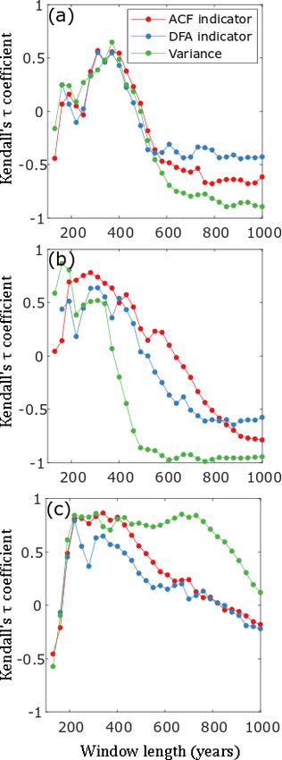
S. H. R. Rosier et al.: Tipping points of Pine Island Glacier                                                                    1505

et al., 2019). Sub-ice-shelf melt rates are increased linearly
(with additional variability as explained below) from a value                            2
that generates a steady state for the present-day glacier con-                    ρw cp
                                                                   M = f γT                    (T0 − Tf ) |T0 − Tf | ,             (1)
figuration. Based on the numerical experiments we then eval-                      ρi Li
uate EWIs to test for critical slowing down.                       where γT is the constant heat exchange velocity, ρw is sea-
                                                                   water density, cp is the specific heat capacity of water, ρi is
3.1   Model description
                                                                   ice density, Li is the latent heat of fusion of ice, T0 is the ther-
All simulations use the community Úa ice-flow model                mal forcing and Tf is the freezing temperature (Favier et al.,
(Gudmundsson et al., 2012; Gudmundsson, 2013, 2020),               2019). Melt rates are only applied beneath fully floating ele-
which solves the dynamical equations for ice flow in the           ments to ensure that no melting can possibly occur upstream
shallow-ice-stream approximation (SSTREAM or SSA; Hut-             of the grounding line (Seroussi and Morlinghem, 2018). The
ter, 1983). Bedrock geometry for the PIG domain is a com-          initial melt rate factor (f ) is chosen such that the model finds
bination of the R topo2 dataset (Schaffer et al., 2016) and,       a steady state with a grounding line approximately coincident
where available, an updated bathymetry of the Amundsen             with its position as given in Bedmap2 (Fretwell et al., 2013).
Sea embayment (Millan et al., 2017). Surface ice topogra-          This melt rate factor is the aforementioned control parame-
phy is from CryoSat-2 altimetry (Slater et al., 2018). Depth-      ter that drives changes in the model, some of which may be
averaged ice density is calculated using a meteoric ice den-       identifiable as tipping points.
sity of 917 kg m−3 together with firn depths obtained from             To effectively extract information about the system’s re-
the RACMO2.1 firn densification model (Ligtenberg et al.,          covery time using the statistical methods outlined in Sect. 2,
2011). Snow accumulation is a climatological record ob-            we need to perturb the model in a way that has some measur-
tained from RACMO2.1 and constant in time (Lenaerts et             able impact on the system state. A slow and monotonically
al., 2012).                                                        increasing forcing would make our chosen approach imprac-
   Viscous ice deformation is described by the Glen–               tical and is arguably as unrealistic as a stepwise perturbation.
Steinemann flow law ε̇ = AτEn with exponent n = 3, and             We therefore add natural variability to the linearly increasing
basal motion is modelled using a Weertman sliding law ub =         melt rate factor (f ). There is strong evidence that the inferred
Cτbm with exponent m = 3. The constitutive law and the slid-       and observed changes in PIG over the last century can be
ing law use spatially varying parameters for the ice rate factor   linked to changes in thermocline depth of the Amundsen Sea
(A) and basal slipperiness (C), respectively, to initialise the    shelf, which in turn is influenced by an atmospheric Rossby
model with present-day ice velocities. These are obtained via      wave train originating in the Pacific Ocean (Jenkins et al.,
optimisation methods using satellite observations of surface       2018). Following Jenkins et al. (2018), we use a ∼ 130-year
ice velocity from the Landsat 8 dataset (Scambos et al., 2016;     time series of central tropical Pacific sea surface temperature
Fahnestock et al., 2016). An optimal solution is obtained by       anomalies as a proxy for relevant variability in our melt rate
minimising a cost function that includes both the misfit be-       forcing. We create an autoregressive (AR) model-based sur-
tween observed and modelled velocities and regularisation          rogate from this time series using the Yule–Walker method to
terms. An additional term in the cost function penalises initial   fit the AR model and minimum description length to deter-
rates of ice thickness change in order to ensure that these are    mine the maximum order of the model. This new surrogate
close to zero at the start of simulations. This approach helps     time series has the same decadal variability that would be
to provide a steady-state configuration of PIG from which we       expected for the melting beneath PIG and can be extended to
can conduct our perturbation experiments.                          any length required. As shown in more detail below, by su-
   The Úa model solves the system of equations with the            perimposing this signal onto the linearly increasing melt rate
finite-element method on an unstructured mesh, generated           factor we ensure that the system response contains sufficient
with MESH2D (Engwirda et al., 2014). The mesh remains              variability to extract information about critical slowing down
fixed throughout the simulation to avoid contaminating the         and thereby enable the calculation of EWIs. Furthermore,
time series with errors resulting from remapping fields onto       using natural variability enables us to test the versatility of
a new mesh. The mesh is refined in regions of high strain rate     EWIs if they were to be applied directly to observations.
gradients and fast ice flow as well as around the grounding
                                                                   3.2   Detecting critical slowing down
line. The region of grounding-line mesh refinement, in which
the average element size is ∼ 750 m, extends upstream suffi-       We have already established the control parameter for our
ciently far so that the grounding line always remains within       model, but another important decision to make is what model
this region until after the final MISI collapse.                   output should be used as a measure of the system state. One
   Basal melt rates are calculated using a widely used, local      choice could be changes in ice volume, since they can be re-
quadratic dependency on thermal forcing:                           lated to sea-level rise and ice sheet model simulations tend
                                                                   to focus on this result. However, ice volume varies very
                                                                   smoothly over time, making it difficult to detect changes

https://doi.org/10.5194/tc-15-1501-2021                                                        The Cryosphere, 15, 1501–1516, 2021
1506 S. H. R. Rosier et al.: Tipping points of Pine Island Glacier
Figure 3. Marine ice sheet instability events for Pine Island Glacier. Shown are (a) grounding-line positions before and after the three MISI-
driven glacier collapses with (b) a zoom-in on the initial events (coloured lines). The colour map indicates initially modelled ice velocity, and
the model domain boundary is indicated by a dashed black contour in panel (a). Panels (c) and (d) show a transect through the main trunk of
PIG, calculated as an average of properties between the two dashed magenta lines in (b). The vertical section along the transect is shown (c)
at the initial steady state where fluxes (Qin and Qout ) are in balance and (d) during a MISI event where retreat causes an increase in Qout ,
pushing the glacier to be out of balance and leading to further retreat.
in the system recovery time. Instead, we use the integrated using the lag-1 auto-correlation function (Dakos et al.,
grounding-line flux, which shows greater temporal variabil- 2008; Scheffer et al., 2009; Held and Kleinen, 2004) ap-
ity and whose change is directly related to the MISI mech- plied to the grounding-line flux over a 300-year moving
anism. As with other studies of this type, the model output window preceding each tipping point (ACF indicator).
is processed prior to the calculation of EWIs. This consists
of aggregating the output (i.e. data binning) to remove vari- 2. Similarly, DFA (Peng et al., 1994) measures increasing
ability with a frequency higher than that directly relevant to auto-correlation in a time series and we apply this with
the internal ice dynamics considered here and thus not re- the same moving-window approach.
lated to the system recovery time, together with detrending
3. An additional consequence of critical slowing down
to remove non-stationarities (detrending is included in the
is that variance will increase as a tipping point is ap-
DFA algorithm and therefore not required before calculation
proached (Scheffer et al., 2009). We calculate variance
of the DFA indicator). Detrending was carried out using a
of grounding-line flux for each moving window, and this
Gaussian kernel smoothing function that has been shown to
can be used in conjunction with other indicators to in-
perform better than linear detrending (Lenton et al., 2012a).
crease robustness.
A smoothing bandwidth was selected that removed long-
term trends without overfitting the model time series. Indi- As described in Sect. 2, recovery time should tend to infin-
cators are calculated over a moving window with a length of ity as a tipping point is approached. This corresponds to the
300 years. The optimal window length is further discussed in ACF and scaled DFA indicators reaching a critical value of
Sect. 4.3. 1. In practice, for a complex model there are a wide variety
From the processed time series, we calculate three differ- of reasons why a tipping point might be crossed before the
ent EWIs: EWI reaches a critical value. For example, this can be a result
of variability in the control variable pushing the system over
1. Critical slowing down is measurable as an increase in a tipping point despite its long-term mean still being some
the state variable auto-correlation. We measure this here distance from its critical value. For this reason, most studies
The Cryosphere, 15, 1501–1516, 2021 https://doi.org/10.5194/tc-15-1501-2021S. H. R. Rosier et al.: Tipping points of Pine Island Glacier 1507
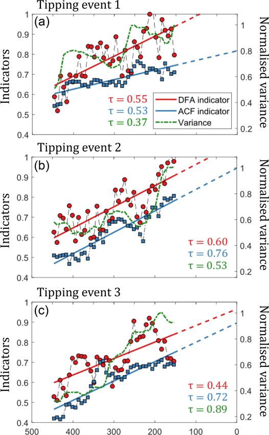
adopt an alternative approach of looking for a consistent in- 4.1 Early warning for the marine ice sheet instability
crease in the EWIs in the run up to a tipping event. This is
often measured by calculating the nonparametric Kendall’s The three periods of MISI-driven retreat, each following the
τ coefficient, a measure of the ranking or ordering of a vari- crossing of an associated tipping point, can be identified
able, which equals 1 if the indicator is monotonically increas- clearly using EWIs (Fig. 5). The ACF indicator increases and
ing with time (Dakos et al., 2008; Kendall, 1948). This sin- tends to 1 as the tipping points are approached (Fig. 5a–c), in-
gle value enables a simple interpretation of our results, since dicating a tendency towards an infinitely long recovery time
0 < τ ≤ 1 means the EWI is tending to increase with time, as predicted by theory. We calculate Kendall’s τ coefficient
suggesting an imminent tipping point. The closer to 1 the to identify trends in the indicator, with a value of 1 repre-
calculated τ coefficient is, the greater the tendency for an in- senting a monotonic increase in the indicator with time. The
dicator to be increasing with time, and conversely a τ coeffi- positive Kendall’s τ coefficient shows that in all three cases,
cient close to zero suggests no clear tendency for an indicator the lag-1 auto-correlation increases before the onset of unsta-
to be changing with time. We present our results in terms of ble retreat. Furthermore, the ACF indicator reaches a critical
both aforementioned criteria: whether an EWI reaches a crit- value of 1 relatively close in time to when the MISI event
ical value preceding the tipping point and whether the EWI is begins.
consistently increasing for a period of time before the tipping These findings are supported by the DFA indicator, de-
point. scribed in Sect. 2. As with the ACF indicator, Kendall’s τ
coefficient is positive and the DFA indicator trends towards
4 Results a critical value of 1 as each tipping point is approached. We
show the change in normalised variance calculated over each
The quasi-equilibrium simulation shows three potential tip- time window, and in all cases this increases ahead of the tip-
ping points with respect to the applied melt (Fig. 4). Upon ping points being crossed with a positive Kendall’s τ coeffi-
crossing each threshold, indicated by the numbered blue dots cient. The increase in variance gives greater confidence to the
in Fig. 4, PIG undergoes periods of not only rapid but also (as findings of the other two EWIs, although variance cannot be
we show below) self-sustained and irreversible mass loss. At used directly to predict when that threshold will be crossed
this stage, relying only on a record of changes in ice vol- since it does not approach a critical value before a tipping
ume resulting from an increasing forcing (solid black line point is crossed.
in Fig. 4), one can only speculate that these are indeed tip-
ping points and more analysis is necessary to confirm this 4.2 Hysteresis of Pine Island Glacier
hypothesis, and we will address this point in Sect. 4.2. The
last of the three events causes a permanently irreversible col-
In order to verify that we have correctly identified tipping
lapse within the entire model domain (Fig. 4a). We focus our
points using the EWIs, we run the model to a steady state
results on these three major changes in the glacier configu-
for a given melt rate to search for hysteresis loops that indi-
ration and ignore any possible smaller tipping points that do
cate the presence of unstable grounding-line positions. These
not result in significant grounding-line retreat or changes in
simulations start from either the initial model setup (advance
ice volume. We increase basal melt rates gradually and in
steady state) or the configuration just prior to the final tip-
a quasi-steady-state manner to ensure that successive retreat
ping point (retreat steady state). Each of these simulations
events can be isolated and their effects do not overlap dur-
samples a discrete mean melt factor between these two states
ing the simulation. A more rapidly increasing forcing could
that is held constant (but with the addition of the same natural
lead to one tipping point cascading into the next and result in
variability as in the forward simulations) and is run forward
three individual tipping points being misinterpreted as only
in time until the modelled ice volume reaches a steady state.
one event.
The first two tipping events show relatively small but clearly
Grounding-line positions before each of these retreat
identifiable hysteresis loops (Fig. 4b), for which recovery of
events and after the final collapse are shown in Fig. 3. Events
the grounding-line position requires reversing the forcing be-
1 and 2 each contribute approximately 20 mm of sea-level
yond the point at which retreat was triggered (i.e. as shown
rise, while event 3, which arises after slightly more than dou-
in Fig. 1c). The third event marks the onset of an almost
bling current melt rates, contributes approximately 100 mm.
complete collapse of PIG (Fig. 4a). Unlike the previous two,
The actual sea-level rise that would result from this third and
this collapse cannot be reversed to regrow the glacier for any
largest event is likely to be larger since in our simulation the
value of the control parameter. This is an example of a per-
effects stop at the domain boundary and in reality neighbour-
manently irreversible tipping point, as shown in Fig. 1d. Note
ing drainage basins would be affected.
that this permanent irreversibility is only true for the glacier
modelled in isolation and by expanding the domain it would
presumably be possible for other catchments that may not
have collapsed to enable this glacier to regrow.
https://doi.org/10.5194/tc-15-1501-2021 The Cryosphere, 15, 1501–1516, 20211508 S. H. R. Rosier et al.: Tipping points of Pine Island Glacier
Figure 4. Change in system state in terms of sea-level equivalent ice volume as a function of the control parameter, which is the melt rate
at the ice–ocean interface. (a) The model is run forward with a slowly increasing basal melt rate (solid black line) and shows three distinct
tipping points (blue dots). From the start of the transient simulation to the third tipping point is approximately 10 kyr. The steady states for a
given melt rate in both an advance and retreat configuration are plotted as dashed grey lines, with details shown in panel (b). Arrows indicate
the direction of the hysteresis. Panel (b) focuses on the model response before the larger tipping point (event 3) and shows the three windows
that we analyse for early warning indicators as shaded red boxes (Fig. 5). Circle and square symbols represent steady-state configurations for
a given forcing, and the dashed grey line is a linear interpolation between these points. Each step in melt rate for the steady-state runs from
∼ 10 to ∼ 30 m a−1 is approximately equivalent to 0.4 m a−1 of basal melting, or 250 years in the transient simulation. The lower branch in
panel (a) represents a simulation starting from the PIG configuration after the third major retreat event and reverses the basal melt rate factor
to its lowest value, showing no recovery in ice volume.
4.3 Robustness of the indicators of 600 years), which is the shortest window size for which
the DFA indicator provides a clear prediction for all tipping
events. We explored the prediction radius of our model by
We carry out several tests to assess the robustness of the calculating Kendall’s τ for the ACF and DFA indicators and
EWIs and their sensitivity to the pre-processing carried out the variance for a range of window lengths; see Fig. 7. For the
on the model output prior to calculating each indicator. Two main tipping event, preceded by the longest stable period, the
parameters in this processing step are the bin size into which indicators gradually lose their ability to anticipate a tipping
data are aggregated and the bandwidth of the smoothing event. This is shown by Kendall’s τ values approaching zero
kernel that removes long-term trends in the time series. To or in some cases becoming negative, meaning that the EWIs
check that the increasing trends in our indicators are a ro- are not robustly increasing before each tipping point as a re-
bust feature of our results, regardless of these choices, we sult of more data being included further from the bifurcation.
conducted a sensitivity analysis. The parameters were var- The same is true for the two smaller tipping events, but the
ied by ±50 %, and the indicators were recalculated for each drop-off is quicker such that the indicators break down for
resulting time series. As before, we assess the utility of an in- window lengths > 500 years. These results suggest that the
dicator by whether it shows an increasing trend before each prediction radius is relatively small, and thus window sizes
tipping point, as measured by a positive Kendall’s τ coef- that are too large, which hence include data far from a tip-
ficient. The results of this sensitivity analysis are presented ping point, become less useful for the application of EWIs.
for each MISI event in Fig. 6. Kendall’s τ coefficient is pos- In addition to a sensitivity analysis, it is important to check
itive for all tested combinations of parameters and all MISI that trends in the calculated indicators are statistically sig-
events, although MISI event 2 is particularly insensitive to nificant and not the result of random fluctuations. We fol-
these parameter choices, whereas the spread in Kendall’s τ low the method originally proposed by Dakos et al. (2012)
coefficient is greater for the other two events. and produce surrogate datasets from the model time series
In general, critical slowing down will only occur close to that have many of the same properties but should not con-
a tipping point. Determining how close to a tipping point a tain any critical-slowing-down trends. We generate 1000 of
system must be in order to anticipate the approaching critical these datasets using an autoregressive AR(1) process-based
transition, i.e. the prediction radius, is an important question surrogate. For each of these datasets we calculate the ACF
and also informs the selection of palaeo-records that could be and DFA indicators and variance in the same way as with
used to detect an upcoming MISI event. The results presented the model time series and then estimate the trend with val-
above are for a window size of 300 years (i.e. a record length
The Cryosphere, 15, 1501–1516, 2021 https://doi.org/10.5194/tc-15-1501-2021S. H. R. Rosier et al.: Tipping points of Pine Island Glacier 1509
Figure 6. Sensitivity analysis for the ACF and DFA indicators. Each
occurrence is Kendall’s τ coefficient for a different choice of filter-
ing bandwidth and data aggregation. The solid red and blue lines
show Kendall’s τ coefficient for the DFA and ACF indicators, re-
spectively, as calculated for the choice of parameters used in Fig. 5.
lation with gradually increasing melt rates. Tipping points
driven by MISI represent potential “high-impact” shifts in
Figure 5. EWIs for the marine ice sheet instability in Pine Island the Earth climate system, since they may lead to considerable
Glacier. Each panel shows the EWIs preceding each of the three changes in the configuration of the Antarctic Ice Sheet that
MISI tipping-point events marked in Fig. 3b, along with the linear
are effectively irreversible on human timescales. Computa-
trend extrapolated to the point in the simulation when the respective
tipping event occurs. Increasing trends in all indicators are shown
tional models are frequently used to forecast future changes
by a positive Kendall’s τ coefficient which measures the correlation in the Antarctic Ice Sheet in response to various greenhouse
between each indicator and time at between −1 and 1. gas emission and warming scenarios. Predictive studies of
this kind sometimes label periods of rapid retreat as “unsta-
ble” without further analysis of the type performed here (e.g.
ues of Kendall’s τ coefficient. We calculate the probability Joughin et al., 2014; Ritz et al., 2015; Favier et al., 2014)
of our results being a result of chance for each indicator and or avoid making this diagnosis altogether (DeConto and Pol-
for all three combined as the proportion of cases for which lard, 2016). Here, we have demonstrated that EWIs robustly
the surrogate dataset was found to have a higher correlation approach critical thresholds preceding tipping points driven
than the model time series. We find that P < 0.1 in all but by MISI. Our results show that EWIs can be used as a method
one instance for the ACF and DFA indicators but variance to identify instabilities without the need for the aforemen-
trends were generally less significant (Table 1). However, tioned modelling approach based on computationally expen-
the combined probability that all three indicators would be sive equilibrium simulations.
equally positive as a result of chance was less than 0.02 for It is important to clearly understand what critical thresh-
the first MISI event and less than 0.005 for the second and old is identified by the EWIs. In Fig. 4 the simulated steady
third events. states show the crossing of the tipping point earlier than iden-
tified by the indicators in the transient simulation. Since the
timescales of ice flow are longer than the forcing timescale,
5 Discussion the ice sheet system modelled here does not evolve along
the steady-state branch (as shown schematically in Fig. 1c).
The indicators we have tested provide early warning of tip- Relaxation to a steady state takes centuries to millennia in
ping points as they are approached in our transient simu- the simulations. This means that while technically the crit-
https://doi.org/10.5194/tc-15-1501-2021 The Cryosphere, 15, 1501–1516, 20211510 S. H. R. Rosier et al.: Tipping points of Pine Island Glacier
Table 1. Probability of Kendall’s τ correlation for each indicator being a result of chance. A total of 1000 surrogate time series of the state
variable are generated, and the indicators and Kendall’s τ correlations are calculated for each one. The probability of Kendall’s τ value is
then the fraction of these surrogate time series with a higher correlation coefficient. The total probability is the fraction of surrogates for
which all three indicators have a higher correlation coefficient than is observed in the original model time series.
Event number Indicator name Indicator value Probability Total probability
MISI event 1 DFA 0.55 0.041 0.0198
ACF 0.53 0.122
Variance 0.37 0.315
MISI event 2 DFA 0.60 0.022 0.0030
ACF 0.76 0.012
Variance 0.53 0.207
MISI event 3 DFA 0.44 0.099 0.0044
ACF 0.72 0.026
Variance 0.89 0.018
ical value of the control parameter (basal melt rate) might Secondly, the predictive power of this method decreases as
have already been crossed, the glacier could return to its pre- the distance to tipping increases and must eventually break
vious state in the transient simulation at that point if the basal down altogether. This effect can be clearly seen in Fig. 7
melt rate was reduced below the critical threshold. This is as Kendall’s τ coefficient decreases with increasing window
true until the system state variable crosses its critical value length. Thirdly, there is a risk of so-called “false alarms” and
(point xt in Fig. 1c) – and this is the point identified by the “missed alarms” (Lenton, 2011). False alarms, whereby a
EWIs. This complication in interpreting EWIs is inherent to positive trend in an indicator that is incorrectly interpreted
ice dynamics because of its long response timescales. as a tipping point being imminent, can occur for a wide va-
We find that both the ACF and the DFA indicators not riety of reasons. First and foremost, interpreting EWIs re-
only increase as a tipping point is approached, as shown by quires robust statistical analysis and judicious data process-
positive Kendall coefficients, but also generally approach the ing to ensure that the response time being measured is that
critical value of 1, although with varying degrees of preci- of the critical mode (Lenton, 2011). It is possible that rising
sion (Fig. 5). This enhances their predictive power, since by auto-correlation is a result of other processes, and using more
extending a positive trend line it is possible to approximate than one indicator together with changes in variance can help
what value of the control parameter will eventually cause a mitigate this risk (Ditlevsen and Johnsen, 2010). It is also
tipping point to be crossed. While our experiments in Ap- possible for a tipping point to be crossed with no apparent
pendix A showed that critical slowing down can accurately warning i.e. missed alarms. This could happen if the internal
predict onset of tipping points in an idealised setup, apply- variability in a system is high so that it changes state before
ing this method to a more complex case study may fail, and a bifurcation point is reached or similarly if the forcing is too
in this context our finding that these indicators largely re- sudden. This last point is particularly pertinent, since we in-
tain their predictive power is very encouraging. One area of tentionally perturb our model slowly and do not explore how
additional complexity in our model of PIG compared to the a change in forcing rate affects the performance of our cho-
setup in Appendix A is the bed geometry, which is obtained sen EWIs. Increasing the forcing rate might present further
from observations and so is much less smooth than the syn- difficulties in identifying tipping points by leading to multi-
thetic retrograde bed used in the MISMIP experiments. We ple tipping points being crossed coincidentally. Since in our
explored how the addition of “bumpiness” to bed geometry methodology the control parameter is not held constant after
affects the performance of EWIs and found that it reduces a tipping point is crossed, then if that parameter changes suf-
how clearly we can resolve the change in response time (Ap- ficiently during the time it takes for one tipping event to con-
pendix A). This effect may account for the fact that EWIs do clude, it might reach a second threshold while the first event
not precisely reach a value of 1 at the bifurcation point, but is still underway, disguising the fact that two distinct tipping
confirming this would require further testing. points have been crossed. Changing the control parameter
There are several important caveats to the use of EWIs as very slowly alleviates this issue, since it will only have al-
presented here. Firstly, and as explained above, the tipping tered slightly during the time it takes for a tipping event to
point identified is that of the transient system not in a steady happen. This issue, along with the related issue of cascading
state. Although the transient behaviour is arguably of greater tipping points, is one that we try to avoid in our experiments
societal relevance and an ice sheet is unlikely to ever truly to simplify the analysis but is known to influence EWI per-
be in a steady state, this is an important distinction to make. formance (Dakos et al., 2015; Brock and Carpenter, 2010).
The Cryosphere, 15, 1501–1516, 2021 https://doi.org/10.5194/tc-15-1501-2021S. H. R. Rosier et al.: Tipping points of Pine Island Glacier 1511
yond the simulation. Alternatively, it may be possible to use
this method on observational data, palaeo-records or some
combination thereof. This raises the question of what data
might qualify as useful for the application of EWIs, which
can be broken down further into (1) the type of data needed
and (2) the length of record necessary. As mentioned previ-
ously, ice volume or related measures of an ice sheet’s size
do not show sufficient variability for information on the re-
covery time to be extracted. Ice speed however can change
significantly over very short timescales; for example many
ice streams show large variability over timescales as short as
tidal periods (Anandakrishnan and Alley, 1997; Gudmunds-
son, 2006; Minchew et al., 2017). Ice flux was chosen in this
study since it is closely related to the MISI mechanism and
because flux is proportional to velocity, but it is possible that
other metrics related to ice velocity might also exhibit critical
slowing down in a similar way. With regards to record length,
we find in this study that early warning of tipping points be-
comes less reliable (with a low or even negative Kendall’s
τ coefficient) for a moving-window size shorter than 200–
300 years. However, this does not mean that this represents
the minimum window size in general and is likely sensitive
to a number of the choices in our methodology. For example,
this value is likely to be sensitive to the rate of forcing applied
to the system. In the limiting case of a forcing rate approach-
ing zero, the necessary window length must increase since
EWIs are only expected to work relatively close to the tip-
ping point. Both of these points require further study in order
to establish suitable datasets for prediction of MISI onset.
6 Conclusions
Conducting quasi-steady numerical experiments, whereby
the underside of the PIG ice shelf is forced with a slowly
increasing ocean-induced melt, we have established the ex-
Figure 7. The effect of window length on the predictive power of istence of at least three distinct tipping points. Crossing
EWIs for MISI. The three panels show the change in Kendall’s τ each tipping point initiates periods of irreversible and self-
coefficient as calculated for each indicator versus window length sustained retreat of the grounding line (MISI) with signifi-
for MISI events 1, 2 and 3 (panels a, b and c, respectively). cant contributions to global sea-level rise. The tipping points
are identified through critical slowing down, a general be-
havioural characteristic of non-linear systems as they ap-
Despite our use of a very slow forcing rate, it is possible that proach a tipping point. EWIs have been successfully applied
more than three tipping points exist in our model configu- to detect critical slowing down in other complex systems.
ration. Finding all possible tipping points would necessitate We show here that they robustly detect the onset of the ma-
infinitesimally small changes in the control parameter, in ei- rine ice sheet instability in the simulations of the realistic
ther the steady-state or the transient simulations, greatly in- PIG configuration which is promising for application of early
creasing computational cost but with little benefit in terms of warning to further cryospheric systems and beyond. While
detecting tipping events that constitute substantial mass loss. the possibility of PIG undergoing unstable retreat has been
In this paper we have presented an application of EWIs to raised and discussed previously, this is to our knowledge the
model output to anticipate tipping points. This is a useful ap- first time the stability regime of PIG has been mapped out
proach in and of itself, since it could be used in model studies in this fashion. The first and second tipping events are rel-
to detect bifurcations in the system with minimal computa- atively small and could be missed without careful analysis
tional expense or to check whether a model might be on a of model results but nevertheless are important in that they
trajectory to cross a tipping point at some point in time be- lead to considerable sea-level rise and would require a large
https://doi.org/10.5194/tc-15-1501-2021 The Cryosphere, 15, 1501–1516, 20211512 S. H. R. Rosier et al.: Tipping points of Pine Island Glacier reversal in ocean conditions for recovery. The third and final tipping point is crossed with an increase in sub-shelf melt rates equivalent to a +1.2 ◦ C increase in ocean temperatures from initial conditions and leads to a complete collapse of PIG. Long-term warming and shoaling trends in Circumpo- lar Deep Water (Holland et al., 2019), in combination with changing wind patterns in the Amundsen Sea (Turner et al., 2017), can expose the PIG ice shelf to warmer waters for longer periods of time and make temperature changes of this magnitude increasingly likely. The Cryosphere, 15, 1501–1516, 2021 https://doi.org/10.5194/tc-15-1501-2021
S. H. R. Rosier et al.: Tipping points of Pine Island Glacier                                                                        1513

Appendix A: Flow line experiments

MISI has been a major focus of modelling efforts within the
glaciological community in recent years. In an effort to as-
sess how ice-flow models capture this behaviour, a model
inter-comparison experiment was performed to calculate the
hysteresis loop of advance and retreat of a marine ice sheet
on a retrograde slope, known as MISMIP experiment 3 (re-
ferred to as EXP 3 hereafter; Pattyn et al., 2012). As a first
step to establishing whether critical slowing down can be ob-
served prior to MISI, we undertook a slightly modified ver-
sion of this experiment using the Úa ice-flow model (Gud-
mundsson, 2012, 2013; see Methods). In our modified exper-
iment, the marine ice sheet is forced towards tipping points
through step perturbations in the control parameter as before
but with smaller steps and the additional constraint that the
model must be in a steady state after each perturbation be-
fore moving on to the next. In this experiment the chosen
control parameter is the ice rate factor, a parameter linked to
ice viscosity and temperature.
   Following each perturbation in the ice rate factor, we anal-
yse the e-folding relaxation time (TR ) of the state variable (in
this case, grounding-line position) to directly extract the re-
covery time of the model as it approaches each tipping point
(both advance and retreat). Theory predicts that TR → ∞
close to a tipping point and that the point at which TR−2 (as
plotted versus the control parameter) reaches 0 thus identifies
the critical value of the control parameter, beyond which a
                                                                    Figure A1. Results of EXP 3, showing change in grounding-line
tipping point is crossed (Wissel, 1984). We show this plot for      position with time resulting from step perturbations in the ice rate
both the advance and retreat scenarios of EXP 3 in Fig. A1.         factor (a). The calculated inverse relaxation time for each corre-
In both cases the relaxation time increases (TR−2 decreases)        sponding step change in rate factor in both the advance (square sym-
as predicted by theory, even far from the tipping point. A lin-     bols) and retreat (circular symbols) phase is shown in panel (b). The
ear fit through the last six perturbations yields a good agree-     dashed line in panel (b) is a line of best fit, calculated for the five
ment with theory and accurately predicts the critical value of      steps in rate factor that preceded the advance or retreat MISI phase.
the control parameter when compared to the analytical solu-         Red arrows indicate the rate factors for which the analytical solu-
tion (red arrows in Fig. A1) given by Schoof (2007). Critical       tion predicts a MISI event, and black arrows show the direction of
slowing down still occurs outside of this range (equivalent to      the forcing towards each tipping point.
a change in ice temperature of > 5 ◦ C), but using these more
distant points to forecast the tipping point would yield a less
                                                                    the persistence. We made the common choice of a lacunarity
accurate prediction. These results therefore provide some in-
                                                                    greater than 1 and a persistence less than one, meaning that
sight into how far from the tipping point we can expect the
                                                                    each octave adds noise of a higher frequency and lower am-
predicted linear response.
                                                                    plitude. For a starting octave amplitude of 25 m the difference
   One major simplification in this idealised experiment is the
                                                                    between the analytical solution and linear fit is less than 1 %,
bed geometry, which is synthetic and arguably unrealistically
                                                                    but this grows to ∼ 5 % with an amplitude of 50 m (note the
smooth. To test whether the addition of bumpiness to the bed
                                                                    change in height from peak to trough in the retrograde region
affects how accurately the critical value of the control pa-
                                                                    of the smooth bed is ∼ 120 m). This suggests that more re-
rameter can be predicted, we conducted further experiments
                                                                    alistic bed geometries with increased roughness might make
in which the bed was made successively less smooth. One
                                                                    the task of predicting tipping points more challenging than it
simple but flexible way to generate the desired roughness is
                                                                    is in this simplified case.
to add Perlin noise to the bed. Perlin noise is a commonly
used method in terrain generation that adds noise at a num-
ber of levels with successively smaller wavelengths and am-
plitudes. The number of levels is denoted by the octave; the
rate at which each octave changes frequency is the lacunar-
ity, and the rate at which each octave changes amplitude is

https://doi.org/10.5194/tc-15-1501-2021                                                     The Cryosphere, 15, 1501–1516, 2021
You can also read