Phenotypic-dependent variability and the emergence of tolerance in bacterial populations
←
→
Page content transcription
If your browser does not render page correctly, please read the page content below
Phenotypic-dependent variability and the emergence of
                                                             tolerance in bacterial populations
                                                             José Camacho Mateu1, ¶ , Matteo Sireci2, ¶ , Miguel A. Muñoz1, * ,

                                                             1 Departamento de Matemáticas, Universidad Carlos III de Madrid, Leganés, Spain
                                                             2 Departamento de Electromagnetismo y Fı́sica de la Materia and
                                                             Instituto Carlos I de Fı́sica Teórica y Computacional. Universidad de Granada.
arXiv:2109.08416v1 [q-bio.PE] 17 Sep 2021

                                                             Granada, Spain

                                                             ¶ These authors contributed equally to this work.
                                                             * mamunoz@onsager.ugr.es

                                                             Abstract
                                                             Ecological and evolutionary dynamics have been historically regarded as unfolding at
                                                             broadly separated timescales. However, these two types of processes are nowadays
                                                             well-documented to intersperse much more tightly than traditionally assumed, especially
                                                             in communities of microorganisms. Advancing the development of mathematical and
                                                             computational approaches to shed novel light onto eco-evolutionary problems is a
                                                             challenge of utmost relevance. With this motivation in mind, here we scrutinize recent
                                                             experimental results showing evidence of rapid evolution of tolerance by lag in bacterial
                                                             populations that are periodically exposed to antibiotic stress in laboratory conditions.
                                                             In particular, the distribution of single-cell lag times —i.e., the times that individual
                                                             bacteria from the community remain in a dormant state to cope with stress— evolves
                                                             its average value to approximately fit the antibiotic-exposure time. Moreover, the
                                                             distribution develops right-skewed heavy tails, revealing the presence of individuals with
                                                             anomalously large lag times. Here, we develop a parsimonious individual-based model
                                                             mimicking the actual demographic processes of the experimental setup. Individuals are
                                                             characterized by a single phenotypic trait: their intrinsic lag time, which is transmitted
                                                             with variation to the progeny. The model —in a version in which the amplitude of
                                                             phenotypic variations grows with the parent’s lag time— is able to reproduce quite well
                                                             the key empirical observations. Furthermore, we develop a general mathematical
                                                             framework allowing us to describe with good accuracy the properties of the stochastic
                                                             model by means of a macroscopic equation, which generalizes the Crow-Kimura
                                                             equation in population genetics. Even if the model does not account for all the
                                                             biological mechanisms (e.g., genetic changes) in a detailed way —i.e., it is a
                                                             phenomenological one— it sheds light onto the eco-evolutionary dynamics of the
                                                             problem and can be helpful to design strategies to hinder the emergence of tolerance in
                                                             bacterial communities. From a broader perspective, this work represents a benchmark
                                                             for the mathematical framework designed to tackle much more general eco-evolutionary
                                                             problems, thus paving the road to further research avenues.

                                                             Author summary
                                                             Problems in which ecological and evolutionary changes occur at similar timescales and
                                                             feedback into each other are ubiquitous and of outmost importance, especially in

                                        September 20, 2021                                                                                        1/31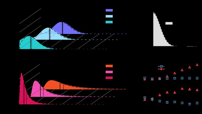
microbiology. A particularly relevant problem is that of the emergence of tolerance to
                     antibiotics by lag, that has been recently shown to emerge very fast in bacterial (E. coli)
                     populations under controlled laboratory conditions. Here, we present a computational
                     individual-based model, allowing us to reproduce empirical observations and, also,
                     introduce a very general analytical framework to rationalize such results. We believe
                     that our combined computational and analytical approach may inform the development
                     of well-informed strategies to mitigate the emergence of bacterial tolerance and
                     resistance to antibiotics and, more generally, can help shedding light onto more general
                     eco-evolutionary problems.

                     Introduction
                     The extraordinary ability of species to adapt and survive in unpredictably-changing and
                     unfavorable environments is certainly one of the most astonishing features among the
                     many wonders of the phenomenon that we call life. Such adaptations can occur at
                     extremely fast temporal scales thus interspersing ecological and evolutionary
                     processes [1–3]. A widely spread surviving strategy is latency or dormancy, i.e., the
                     possibility for organisms to enter a period of reduced metabolic activity and
                     non-replication adopted during adverse environmental conditions [4–8]. Examples of
                     dormancy can be found across kingdoms, with examples ranging from microorganisms
                     such as viruses, bacteria or fungi [9–12] to plants [13, 14] and animals [7]. During the
                     latency period the organism is said to be in a latent or dormant state and the time it
                     takes to wake up is referred to as “lag time” or simply “lag”. Entering and exiting a
                     dormant state are not cost-free processes, since individuals may require of a specific
                     metabolic machinery for performing such transitions and/or the development of
                     specifically-devised “resting structures” [4, 5, 15–17]. The exit from the dormant state
                     can occur either as a response to environmental signals or cues [4, 5, 10, 18] or,
                     alternatively, in a stochastic way [19–23]. As a matter of fact, the duration of the lag
                     intervals often varies widely between conspecific individuals and even between
                     genetically identical organisms exposed to the very same environmental
                     conditions [10, 19, 24, 25]. Such a variability is retained as an example of phenotypic
                     diversification or bet-hedging strategy [26, 27] that confers a crucial competitive
                     advantage in unpredictable and rapidly changing environments, thus compensating the
                     above-mentioned individual costs and providing important benefits to the community as
                     a whole [4, 5, 10, 14, 28, 29].
                         Although, as already stated, latency is a widespread phenomenon, bacterial
                     communities constitute the most suitable playground for quantitative analysis of latency
                     owing to their diversity, fast life cycle, and the well-controlled conditions in which they
                     can grow and proliferate in the laboratory [30–33]. Actually, latency was first described
                     by Müller back in 1895 as an explanation for the observed irregularities in the growth
                     rate of bacterial cultures in his laboratory [34]. In recent years it has been realized that
                     bacterial latency is a more complex and rich phenomenon than previously thought.
                     Indeed, paraphrasing a recent review on the subject, the lag phase is “dynamic,
                     organized, adaptive, and evolvable” [10].
                         Bacterial latency is at the root of tolerance to antibiotics as, rather often,
                     bactericidal antibiotics act during the reproduction stage and thus, by entering a
                     dormant state, bacteria become transiently insensitive to antibiotics. Let us recall that
                     bacterial tolerance is not to be confused with bacterial resistance [35]. While resistance
                     refers to the ability of organisms to grow within a medium with antibiotics, provided
                     these are not in high concentrations, tolerance is the ability to transiently overcome
                     antibiotics, even at very high concentrations, provided the exposition time is not too
                     large [24, 35, 36]. The strengths of these two complementary surviving strategies are

September 20, 2021                                                                                          2/31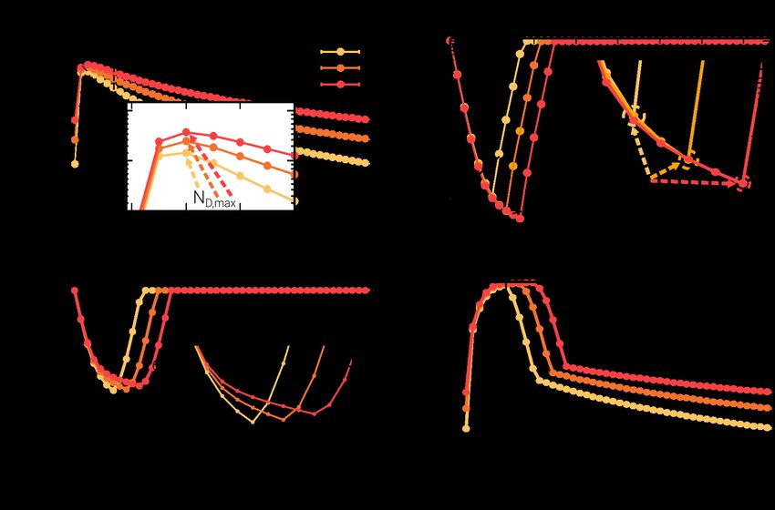
quantified, respectively, in terms of quantities: (i) the minimum inhibitory concentration
                     (MIC) of drug that must be supplied to stop the population growth —a quantity that is
                     significantly increased in resistant strains [24, 25, 35, 37]— and (ii) the minimum
                     duration to kill 99% of the cells M DK99 , which is increased in tolerant strains [38].
                         While the importance of bacterial resistance has long been recognized, studies
                     underlining the crucial role played by tolerance are less frequent and more
                     recent [24, 25, 35, 37]. An important caveat is that, while resistance is specific to one or a
                     few antibiotics, tolerance is generically effective for a large diversity of them, leading to
                     survival even under intensive multidrug treatment [24, 25, 35]. Moreover, there exists
                     firm evidence that tolerance is the first response to antibiotic stress [37], facilitating the
                     later appearance of resistance [25]. Therefore, understanding the emergence of tolerance
                     is crucial for the development of more effective therapies aimed at dealing with
                     recalcitrant infections and possibly preventing them. Aimed at shedding light on these
                     issues, here we present an eco-evolutionary approach to analyze the emergence of
                     tolerance by lag in bacterial communities under controlled laboratory experiments. In
                     particular, we scrutinize the conditions under which modified lag-time distributions
                     evolve as a response to stressful environments and investigate the origin of the
                     experimentally-observed broad heavy tails in lag-time distributions (see below).
                         Beside this specific focus, the present work has a broader breath. The example of
                     rapid evolution of lag-time distributions is used as a test to prove a theoretical
                     framework that we are presently developing. Our framework is similar in spirit to
                     existing approaches such as the theory of “adaptive dynamics” and related models in
                     population genetics [39–42], but aims at reconciling and generalizing them.
                         As a historical sidenote, let us recall that adaptive dynamics (AD) was born as a
                     generalization of evolutionary game theory [43] to allow for a set of strategies that is
                     continuously varying and, upon which selection acts. AD led to the satisfactory
                     explanation of intriguing phenomena such as evolutionary branching [39, 40, 44, 45],
                     speciation [46–48], diversification [49, 50], the emergence of altruism and
                     cooperation [51, 52], and the evolution of dispersal [53]. Importantly, its foundations are
                     also mathematically well-established [54]. However, in spite of its very successful history,
                     AD in its standard formulation has some limitations that make it not directly applicable
                     to complex situations such as the one we aim at describing here:
                         (i) First of all, in its standard formulation, populations are considered as
                     monomorphic, i.e. point-like in phenotypic space; thus it does not allow for
                     phenotypically-structured populations (see however [55, 56]).
                         (ii) The “macroscopic equations” of AD for the populations are not easily connected
                     to microscopic birth-death processes in individual-based models [57].
                         (iii) Variations are assumed to be small, typically Gaussian-distributed and
                     independent of the parent’s phenotypic state.
                         (iv) Variations are considered to be rare: “after every mutational event, the
                     ecological dynamics has time to equilibrate and reach a new ecological attractor” [58].
                     In other words, a separation is assumed between ecological and evolutionary timescales,
                     while in microbial communities, such processes may occur in concomitance. Such a
                     convergence of characteristic timescales is the hallmark of eco-evolutionary
                     dynamics [1–3] and is at the basis of fascinating phenomena such as eco-evolutionary
                     tunneling [58, 59] and other rapid evolutionary phenomena [32, 60–63] which are difficult
                     to account for in the standard formulation of adaptive dynamics.
                         In what follows, we employ a theoretical framework in the spirit of statistical
                     mechanics that aims to fill the gap between theory, phenomenological models and, most
                     importantly, experiments. Thus, our approach —which is similar in spirit to previous
                     work on bacterial quorum-sensing by E. Frey and collaborators [64, 65]— implements a
                     number of extensions with respect to standard AD [66], as it makes explicit the

September 20, 2021                                                                                           3/31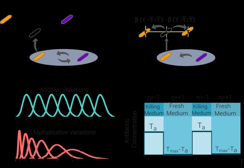
connection between individuals (microscale), and community dynamics (macroscale),
                     introduces a general variation kernel, allows for large and phenotypic-state-dependent
                     variations, etc. These extensions allow us to study phenotypic diversity within a
                     well-characterized eco-evolutionary framework. A full account of this general theoretical
                     framework will be presented elsewhere [67]. Let us finally emphasize that many of the
                     above questions and extensions have been already tackled in the mathematical
                     literature, at a formal level [54, 68]. Yet, to the best of our knowledge, these results have
                     have been confined to rigorous analyses of toy models and have not fully percolated
                     through the biological and physical literature.
                         The paper is organized as follows: in the first section we discuss in detail the
                     experimental setup and empirical findings object of our study; then, we introduce a
                     stochastic individual-based model implementing phenotypic variability and inheritability
                     to account for experimental results. We present an extensive set of both computational
                     and analytical results for it, discussing in particular the conditions under which the
                     mathematical results deviate from computational ones. Finally, we discuss the
                     implications of our work both from a biological viewpoint and how it contributes to the
                     understanding of the evolution of heterogeneous phenotypic distributions, as well as
                     from a more general eco-evolutionary perspective.

                     Empirical observations: rapid evolution of lag-time distributions
                     For the sake of concreteness, we focus on recent experimental results on the rapid
                     evolution of tolerance in populations of Escherichia coli in laboratory batch cultures in
                     Balaban’s lab [24]. In particular, a bacterial population is periodically exposed to
                     antibiotics (amplicillin) in very high concentrations (much larger than the MIC ) during
                     a fixed-duration time interval Ta (e.g., Ta = 3, 5, or 8 hours). After antibiotic exposure
                     the system is washed and the surviving population is regrown in a fresh medium during
                     a time interval T (with T = 23h − Ta ). The antibiotics/fresh-medium cycle is iterated
                     at least 8 or 10 times. Results are averaged over 2 experimental realizations for each Ta
                     and the resulting maximal carrying capacity is about 109 individuals (we refer to [24]
                     for further biological and experimental details).
                         Once the cycles are completed, Fridman et al. [24] isolated some individuals from the
                     surviving community and by regrowing them in a fresh medium they found that the
                     distribution P (τ ) of lag times τ —i.e. the time individual dormant cells take to start
                     generating a new colony after innoculation into a fresh medium— changes from its
                     ancestral shape to a modified one, shifted towards larger τ values. More specifically, the
                     mean value grew to a value that approximately matches the duration of the
                     antibiotic-exposure time interval, Ta (see [24]). This modified lag-time distribution
                     entails an increase in the survival probability under exposure to ampicillin but, also, to
                     antibiotics of a different bactericidal class such as norfloxacin, for the same time period.
                     Furthermore, mutations were identified in diverse genes, some of them known to be
                     related with regulatory circuits controlling the lag-time distribution, such as the
                     toxin–antitoxin one [69]. Subsequently, after many cycles, the population was also
                     observed to develop resistance to ampicillin [24]. Thus, the conclusion is that
                     non-specific tolerance —stemming from lag— emerges in a very rapid way as a first
                     adaptive change/response to antibiotic stress. More in general, these results reveal that
                     the adaptive process is so fast that ecological and evolutionary processes occur at
                     comparable timescales [63, 70–73].
                         The experimentally-determined lag-time distributions reveal another intriguing
                     aspect that —to the best of our knowledge— has not been extensively analyzed so far:
                     their variance is also significantly increased as Ta grows and, related to this, the
                     resulting mean value of the distribution is always larger than its median [74]. This is an
                     indication that, as a matter of fact, the empirically-obtained lag-time distributions are

September 20, 2021                                                                                           4/31
skewed and exhibit heavy tails, including phenotypes with anomalously-large lag times
—much larger than Ta —, especially for large Ta ’s. This observation is surprising as,
under such controlled lab conditions, one could naively expect to find lag-time
distributions sharply peaked around the optimal time value, Ta , since, ideally, the best
possible strategy would be to wake-up right after antibiotics are removed and any
further delay comes at the price of a reduction of the overall growth rate or fitness.
Fridman et al. proposed that the increase in the variance might suggest a past
selection for a bet-hedging strategy in natural unpredictable environments; however,
anomalously-large lag-time values were not present in the original wild-type population.
The authors also suggested that there could be constraints at the molecular level
imposing the mean and the variance of the lag-time distribution to increase
concomitantly [24, 69], a possibility that inspired us and that we will carefully scrutinize
from a theoretical and computational perspective in what follows.
Model building
Aimed at shedding light onto these empirical findings, here we propose an
individual-based stochastic model for phenotypic adaptation in which each single
individual cell can be either in an “awake” or in a “dormant” state [22, 23, 75–77] (see
Fig 1 for a sketch of the model). Mimicking the experimental protocol of Fridman et
al.— a population of such individuals is exposed to alternating adverse and favorable
conditions with durations Ta and 23h − Ta , respectively (a function η(t) labels the
environmental state at any given time t: η(t) = −1 in the presence of antibiotics and
η(t) = +1 in the fresh medium).
The model assumes that each awake cell is able to sense the environment and
respond to it by regulating its state: they can sense the presence of antibiotics and enter
the dormant state at rate s, while such a machinery is assumed to be turned off during
dormancy. In S1 Text, Sec. S5, we also consider a generalization of the model in which
awake individuals can also enter the dormant state as a response to other sources of
stress such as starvation [78]. Indeed, the wake-up is assumed to occur as a result of a
Markovian stochastic process; each individual bacteria i is phenotypically characterized
by its intrinsic typical mean lag time τi meaning that, it wakes up stochastically at a
constant transition rate 1/τi . Therefore, the time t at which a dormant cell actually
resumes growth is a random variable distributed as P (t|τi ) = e−t/τi /τi , with mean value
τi [79, 80]. In the last section we discuss recent alternatives to Markovian processes, i.e.
including some form of “memory”, which can give rise to non-exponential residence
times, to describe this type of waking-up phenomena [81, 82].
Awake individuals are exposed to stochastic demographic processes: they attempt
asexual reproduction (i.e., duplication) at a constant birth rate b and die spontaneously
at rate d (that we fix to 0 without loss of generality). Reproduction attempts are
successful in the fresh medium while, in the presence of antibiotics, they just lead to the
parent’s death and its removal from the community. Following this dynamics, the
population can freely grow, until its size reaches a maximal carrying capacity K. Once
this limit has been reached, the population enters a saturated regime, within which each
new birth is immediately compensated by a random killing (much as in the Moran
process [83]).
Importantly, in parallel with the above demographic processes, the model
implements an evolutionary/adaptive dynamics. The phenotypic state τi of each
successfully dividing individual is transmitted, with possible variation, to its progeny. In
particular, the two offspring resulting from duplication have phenotypic states τi + ξ1
and τi + ξ2 , respectively, where ξ1 and ξ2 are the phenotypic stochastic variations,
sampled from some probability distribution, that we generically call β(ξ; τi ) and that, in
September 20, 2021 5/31the more general case, can be state-dependent, i.e. depend on τi . More specifically, we
implemented two different variants of the model, depending of the standard deviation of
the probability distribution β(ξ; τi ):
• The additive model, with a standard deviation, αA , common to all phenotypes.
• The multiplicative model, with a state-dependent standard deviation, αM τi , for
individuals with intrinsic lag time τi , where αM is a constant (see Methods).
Observe that in the multiplicative case, the larger the parent’s lag time the larger the
possible amplitude of variations, in a sort of rich-get-richer or Matthew-effect
mechanism, well-known in the theory of stochastic processes to generate heavy
tails [84–93]. As a motivation for this choice, let us mention that there is solid evidence
that the genetic circuits involved in the regulation of the lag-time distribution (such as
the toxin-antitoxin one), can indirectly produce this type of fluctuations at the
phenotypic level [69]. Furthermore, similar phenotypic-variation kernels have been
argued to arise from non-linear effects in the way genotypic changes (mutations) are
manifested into phenotypic variability (see e.g. [94, 95]).
Analytical (mean-field) theory
Before delving into computational analyses of the model, let us present a mathematical
framework allowing us to obtain theoretical insight. Readers not particularly interested
in analytical approaches can safely skip this section, and just be aware that it is possible
to mathematically understand all the forthcoming computational results.
The previous Markovian stochastic individual-based model is mathematically defined
as a “many-particle” Master equation ruling the time evolution of the joint
probability-distribution functions for the whole set of all “particles” ( i.e., cells). The
resulting master equation can be simulated computationally by employing the Gillespie
Algorithm (see below and S1 Text, Sec. S2A, for details) [79, 80, 96]. However, as it is
often the case for such many-particle Master equations, it is hard to handle analytically
in an exact way. Thus, in order to gain quantitative understanding beyond purely
computational analyses, here we develop an approximation —which becomes exact in
the limit of infinitely large population sizes [64, 65]— that allows us to derive a
macroscopic (or “mean-field”) description of the stochastic model in terms of the
probability density of finding an individual at any given phenotypic state, τ (i.e. the
“one-particle” probability density). The mean-field approach that we employ in what
follows is just a first example of a much more general framework that we will expose in
detail elsewhere [67].
A first step toward the derivation of a macroscopic equation relies on a
marginalization of the many-particle probability-distribution function to obtain a
one-particle probability density (see S1 Text, Sec. S2B). The resulting marginalized
distribution function encapsulates the probability density φ(τ, t) that a randomly
sampled individual at R ∞time t has lag time τ . This probability —that needs to be
normalized, so that 0 φ(τ, t)dτ = 1— can be decomposed in two contributions
φ(τ, t) = φG (τ, t) + φD (τ, t) representing, respectively, the relative fraction of
individuals in growing (G) and dormant (D) states. Observe that these two densities are
not probability distributions and thus they are not normalized to unity separately. In
the limit of infinitely-large population sizes, the evolution of the probability density for
individuals in the growing state, φG (τ, t) is ruled by the following equation (details of
September 20, 2021 6/31the derivation can be found in SI, S2A):
Z ∞
1 + η(t)
∂t φG (τ, t) = −bφG (τ, t) + 2b dτ̃ β(τ − τ̃ ; τ̃ )φG (τ̃ , t)
2 0
Z ∞
− bφG (τ, t) dτ̃ φG (τ̃ , t)
0 Z ∞
1 − η(t) 1
− b 1− dτ̃ φG (τ̃ , t) + s φG (τ, t) + φD (τ, t). (1)
2 0 τ
Even if this equation might look cumbersome, its different terms have a rather intuitive
interpretation:
• In the fresh medium (terms proportional to 1 + η(t)): (i) the first term represents
the negative probability flow stemming from growing individuals with generic
phenotypic trait τ that reproduce (at rate b) and change to any other arbitrary
phenotypic state; (ii) the second represents the positive contribution of
reproducing individuals (at rate b) with any arbitrary trait τ̃ , for which one of the
two resulting offspring jumps to τ (controlled by the function β(τ − τ̃ ; τ̃ )); (iii)
the third selection term stems from the normalization of the overall probability
density: if the population size grows because any individual with arbitrary trait τ̃
reproduces successfully (at rate b), then the relative probability to observe
phenotype τ decreases to keep the overall probability-density conserved.
• In the presence of antibiotics (terms proportional to 1 − η(t)): (i) the first term
represents the rate at which growing individuals that attempt reproduction (at
rate b) are killed by antibiotics; (ii) the second term is a selection term, fully
analogous to the above-discussed one: when any arbitrary individual dies the
overall probability density at τ increases; (iii) the third term represents the
outflow of individuals entering the dormant state at rate s.
• In both environments (no dependence on η(t)): the only term, proportional to the
rate 1/τ , describes the probability inflow stemming from dormant individuals that
become awake.
Similarly, the equation for the density of individuals in the dormant state is
Z ∞
1 1 − η(t)
∂t φD (τ, t) = −η(t)bφD (τ, t) dτ̃ φG (τ̃ , t) − φD (τ, t) + sφG (τ, t) (2)
0 τ 2
where the first (selection) term stems from the overall probability conservation when the
population either grows or shrinks (negative or positive signs, respectively), and the
remaining two terms have the opposite meaning (and signs) of their respective
counterparts in Eq.(1).
In order to make further analytical progress, in the case in which variations are
assumed to be small, it is possible to introduce a further (“diffusive” or “Kimura”)
approximation as often done in population genetics as well as in adaptive or
evolutionary mathematical approaches [97]. More specifically, one can perform a
standard (Kramers-Moyal) expansion of the master equation by assuming that jumps in
the phenotypic space are relatively small [79, 80], i.e. expanding the function beta in
Taylor series around 0. After some simple algebra (see S1 Text, Sec. S3) one obtains a
particularly simple expression for the overall probability distribution:
η(t) f (τ, t) − f¯(t) φ(τ, t)
∂t φ(τ, t) =
1
− (η(t) + 1) ∂τ θ(τ )f (τ, t)φ(τ, t) − ∂τ2 σ 2 (τ )f (τ, t)φ(τ, t) (3)
2
September 20, 2021 7/31R ∞ fitness function” f (τ, t) ≡ bφG (τ, t)/φ(τ, t) and its population
where the “ effective
average f¯(t) = 0 dτ f (τ, t)φ(τ, t) have been introduced, and where θ(τ ) and σ 2 (τ ) are
the first and second cumulants of the variation function β (in first approximation we
can assume θ(τ ) = 0, while σ 2 (τ ) = αA
2
for the additive case and σ 2 (τ ) = αM
2 2
τ for the
multiplicative case). Observe that, remarkably, this last equation is a generalization of
the celebrated continuous-time Crow-Kimura equation of population genetics [98], also
called selection-mutation equation [99, 100]. In particular, notice that the dynamics of
the probability density is exposed to the combined action of the process of selection
(first term in Eq.(3), which is nothing but the replicator equation [43, 101]) and
mutation, as specified by the drifts in the second line. This type of equations,
combining replicator dynamics with Fokker-Planck type of terms —even if with a
slightly different interpretation— have been also studied by Sato & Kaneko and Mora &
Walzak [102–104]. The main —and crucial— differences between Eq.(3) and the
standard Crow-Kimura equation are:
• The fitness function appears in the mutation terms —whereas in the standard
Crow-Kimura equation the diffusion term would read ∂τ2 φ(τ )— thus correlating
reproduction rates and mutation amplitudes. Observe that here variations are
always associated with reproduction events, as typically in bacteria and viruses, in
such a way that a higher fitness rate implies a higher mutation rate.
• There is a general dependence on the cumulants of the variation kernel that, in
general, can be trait-dependent and asymmetric.
These generalizations are essential ingredients to capture the essence of our Markovian
model as we will see and, to the best of our knowledge, have not been carefully analyzed
in the past. From here on, we refer to Eq.(3) as the generalized Crow-Kimura (GCK)
equation.
Results
In order to scrutinize whether the proposed adaptive stochastic model can account for
the key empirical findings of Fridman et al. [24], we perform both (i) extensive
computational simulations and (ii) numerical studies of the mean-field macroscopic
equation, Eq.(3).
• Computational simulations rely on the Gillespie algorithm [96], which allows us to
simulate exactly the master equation defining the stochastic model. In all cases,
we consider at least 103 independent realizations to derive statistically-robust
results. Without loss of generality and owing to computational costs, the maximal
population size or carrying capacity is fixed to K = 105 .
• On the other hand, for analytical approaches, in spite of the relatively simple form
of Eq.(3) owing to its non-linear nature and to the time-variability of
environmental conditions η(t), it is not possible to solve it analytically in a closed
way and, thus, it becomes mandatory to resort to numerical-integration schemes.
In particular, from this equation —or, more precisely, from integration of its two
additive components: Eq.(1) and Eq.(2)— one can derive the time-dependent as
well as the asymptotic lag-time distributions and, from them, monitor the leading
moments or cumulants as a function of time.
Further details of both computational simulations and numerical integration of the
macroscopic equation can be found in the Methods section as well as in the S1B. In what
follows we present together both types of analyses, underlining where the mean-field
approach works well and where its predictions deviate from direct simulations.
September 20, 2021 8/31Transient dynamics: determining variational amplitudes
Parameter values in the model are fixed to agree as much as possible with the empirical
ones measured by Fridman et al. [24] (see Methods). In particular, we used (i) the same
set of environmental-period durations Ta and Tmax − Ta as in the
antibiotics/fresh-medium cycle, (ii) the experimentally measured reproduction rate in
the fresh medium, (iii) the empirical “falling-asleep” rate s, as well as (iv) the same
number of antibiotic cycles (ten) as in the experimental setup. Initially all individuals
are assumed to have small intrinsic lag-time values of τ . In particular, we consider a
truncated normal distribution with mean value and variance as in the actual ancestral
population in the experiments (hτ iexp. = 1.0 ± 0.2 h).
Employing this set of experimentally-constrained parameter values and initial
conditions, we ran stochastic simulations in which the whole population expanded and
then shrank following the periodically alternating environments. Along this dynamical
cyclic process the distribution of τ values across the population varies in time; in
particular, we monitored the histogram of τ values and obtained the corresponding
probability distributions right at the end of each antibiotic cycle, just before regrowth,
as in the experiments.
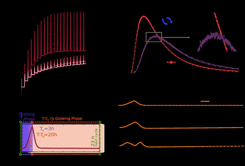
Fig 2A and 2B show the evolution of the mean (i.e. the first cumulant, K1 ) across
cycles, while Fig 3A and 3B illustrate the full distribution and higher-order cumulants
after 10 cycles. Observe that the value of K1 after 10 cycles depends on the choice
made for the only remaining free parameter, i.e. the variation-amplitude parameter αA
or αM , for the additive or multiplicative versions of the model, respectively. In order to
tune either of these parameters, we imposed that K1 (10) reproduces in the closest way
the experimentally determined values, as measured right before the 10th regrowth cycle.
This tuning procedure leads to αA = 0.16(1)h and αM = 0.048(1) for the additive and
multiplicative cases, respectively (parentheses indicate uncertainty in the last digit);
these are the values that best reproduce the empirical findings in the sense of
least-square deviation from the available empirical data for different Ta ’s (see Fig 2C).
Let us remark that both variants of the model are able to reproduce the key
experimental feature of generating mean lag times close to Ta (observe, however, that
there is always a small deviation in the case Ta = 8 h, for which even experimentally,
K1 ≈ 10 h > Ta ). Nevertheless, as illustrated in Fig 3A and 3B there are significant
differences between the two variants. In particular, the additive model fails to reproduce
the following empirical observations:
• Ta -dependent variances,
• large differences between median and mean values, and
• strongly skewed distributions with large tails.
For instance, in the experiments, for Ta = 8 h, the difference between the mean and
the median is 1.1(1) h while in the additive model is 0.15 h, i.e. about one order of
magnitude smaller. Furthermore, in the experiments, lag times of up to 30 h are
observed, while in the additive model values above ≈ 15 are exponentially cancelled; i.e.
they have an extremely low (negligible) probability to be observed. This is also
illustrated in Fig 3D where the second and third cumulants (variance and skewness) of
the distribution after 10 cycles are plotted as a function of Ta . Observe that both
cumulants remain almost constant, revealing the absence of heavy tails for large values
of Ta .
On the other hand, the multiplicative model is able to reproduce not only the
experimental values of the mean but also —with no additional parameter nor fine
tuning— (i) the existence of large lag-time variances that increase with Ta , (ii) the
above-mentioned large differences between the mean and the median (1.3(1) in this
September 20, 2021 9/31case), as well as (iii) heavily skewed lag-time distributions that strongly resemble the
empirically measured ones (see Fig 2 in Fridman et al. [24]). In particular, lag times of
the order of 30 h have a non-negligible probability to be observed for Ta = 8 h within
the multiplicative version of the model, after 10 cycles. The resulting probability and
the corresponding cumulants (see Fig 3D depend strongly on Ta .
Importantly, the previous results are quite robust against changes in the model. In
particular, if growing cells are allowed to switch to dormancy in response of starvation,
the mean lag time increases, as expected, but the qualitative shape of the lag-time
distribution remains unchanged (see S6 ). Hence, just by modifying accordingly the
parameter α allows one to recover the same conclusions.
As a word of caution let us emphasize that the distributions in Fig 3 are not
obtained exactly in the same way as the experimental ones. The first are distributions
of characteristic times τ (inverse of intrinsic transition rates) while the second are the
actual lag times t measured after regrown in a fresh medium. Actually, the
characteristic time τ , in our model, is just a proxy for the actual time that it takes for
the colony formed by such an individual to be observable or detectable in actual
experimental setups. Below we discuss this issue more extensively as well as the possible
limitations it implies and extensions of the modelling approach to circumvent them.
Let us also underline that Fig 3 reports not only the results of direct simulations but
also the theoretical predictions (dashed lines) derived from numerical integration of the
macroscopic equations for the two different cases. The agreement with simulation
results is remarkably accurate; the origin of the existing small discrepancies will be
analyzed in detail in a forthcoming section.
Thus, the main conclusion of these computational and theoretical analyses is that
state-dependent (multiplicative) variability is needed in order to account for the
empirically observed key features of the lag-time distributions emerging after a few
antibiotic/fresh-medium cycles. Once this variant of the model is chosen, a good
agreement with experimental findings if obtained by fitting the only free parameter: the
amplitude of variations.
Asymptotic state
Even if experimental results are available for a fixed and limited number (10) of
antibiotic-exposition cycles, the already-calibrated model allows us to scrutinize the
possible emergence of asymptotic states after a much-larger number of cycles. In other
words, it is possible to go beyond the experimental limits and analyze the fate of the
population. In this sense, the experimental results can be seen as a “transient
adaptation” to the environment, while the evolutionary cycle would be completed only
when an asymptotic (evolutionary stable) state is reached. Let us remark that the
asymptotic state is necessarily a periodic one, as the phenotypic distributions vary at
different instants of the cycle, i.e. the asymptotic distributions —measured at arbitrary
times within the cycle— exhibit periodic oscillations in its shape, tracking the perpetual
environmental cyclic changes. This is illustrated in Fig 4, showing results obtained by
numerically integrating the macroscopic equations, Eq.(1) and Eq.(2). First of all, it
shows periodic oscillations of the mean lag time K1 ; as shown in panel (A) it first
increases from its initial value K1 = 1 and then, eventually, reaches an oscillatory steady
state. More specifically, as clearly seen in the zoomed plot of panel (B), within the
steady state, the maximum mean value within each cycle is reached right before
antibiotics removal. This is an expected result as in the first part of the cycle, i.e.
during the “killing phase”, the presence of antibiotics induces a selective pressure
towards increasing the mean lag-time value because delaying the exit from the lag phase
provides protection from the antibiotics. On the other hand, in the fresh medium
(growing phase) the selective pressure quickly reduces the mean lag time to foster fast
September 20, 2021 10/31growth and increased fitness. Thus, summing up, the periodic alternation of
environmental conditions induces a stable periodic change in the mean lag-time value.
Actually, it is not only the mean that changes periodically, but the whole probability
distribution that varies cyclically. This is illustrated in Fig 4C and 4D which shows
computational and theoretical results for the lag-time probability distribution and its
first cumulants, K1 , K2 and K3 , for the multiplicative case (similar plots for the
additive case are shown in S1 Text, Sec. S6). Observe, in particular, in panel C, that
the distribution oscillates between two extreme or limiting cases corresponding to the
times of antibiotics inoculation and antibiotics removal, respectively. This effect can be
more vividly seen in the S1 and S2 Videos.
Let us also highlight that the probability distributions exhibit non-Gaussian tails
and are right-skewed. In particular, to make these observations more quantitative, Fig
4D shows the variance, K2 , and the skewness, K3 , along the cycle in the steady state.
Notice also the very-good —though not perfect— agreement between computational
results and theoretical estimates (dashed lines in Fig 4C and 4D).
Furthermore, let us emphasize that, importantly, the amplitude of the variations
—as controlled by the parameter αM (or, similarly, αA for the additive case)— has a
non-trivial effect on both the transient and the asymptotic behavior. In particular, the
value of such amplitude not only affects the mean value of lag times after 10 cycles —as
illustrated by the plateau of the oscillations in Fig 4A and 4B— but also (i) its
asymptotic value, i.e. the mean lag time, (ii) the amplitude of the oscillations across a
cycle in the steady state, and (iii) the relaxation time to the asymptotic state (i.e., the
speed of evolution). This is due to the heavy tails of the distribution: increasing the
amplitude of variations directly increments the variance of lag times, but this also
enlarges the left-skewness of the distribution, feeding-back to the mean value. Therefore,
the eco-evolutionary attractor is shaped both by selection and mutation, departing from
the classical evolutionary scenario, as e.g. in adaptive-dynamics, in which the amplitude
of the variations just affects the variance of the resulting distribution but not the overall
attractor.
Finally, we complement our observations with the population structure dynamics, i.e.
proportion, minimum and maximum of dormant and awake cell numbers, in Fig 5. In
particular, panels (A) and (B) show the abundances of dormant and awake cells as
function of time along an asymptotic cycle. Observe that the number of dormant cells
reaches a maximum, ND,max , after one hour, independently of the antibiotic duration
time Ta , while its height is proportional to this parameter. On the other hand, the
position of minimum of growing cells number, NG,min , scales with Ta and its magnitude
decreases correspondently. In Fig 5 we also show and discuss the dependence the total
number of cells N = NG + ND (panel C) as well as the relative fraction of dormant
individuals along a full cycle in the stationary state (which is reached after onley a few
(three) antibiottic cycles).
For the sake of completeness, let us also emphasize that both versions of the model
are able to generate M DK99 values that grow as a function of the number of antibotic
cycles, converging to an asymptotic-state value; at the end of the tenth cycle
simulations compare well with empirical observations for different values of Ta (see S10
and S11 Figs; observe that the largest difference appears for Ta = 8, a case for which
also K1 deviates slightly from Ta in the experiments).
Deviations between theory and simulations: finite-size effects
Thus far, we have reported results stemming from computational analyses of the
individual based model as well as from numerical integration of the associated
macroscopic theory, i.e. the GCK equation. Small but systematic discrepancies between
September 20, 2021 11/31theory and simulations are evident, see for example Fig 4C and 4D. Let us here discuss
the origin of such differences.
The theoretical approach relies on two different approximations: (i) on the one hand
it considers the small-variation approximation to include just the first two moments of
the variation function (i.e. a diffusion approximation); (ii) on the other hand, in order
to derive the macroscopic GCK equation, one needs to neglect correlations between
individuals, a type of mean-field approximation that, as usual, is expected to be exact
only in the infinite population-size limit [79, 80]. In S1 Text, Sec. S4, we show
computational evidence that the small mutation approximation is not a significant
source of errors; hence, the discrepancies necessarily stem from finite-size effects.
Indeed, in the present experimental set up, there is a bottleneck at the end of each
antibiotics cycle, when there is a small number of surviving individuals, thus limiting
the validity of the mean-field approximation in such a regime. As a matter of fact, one
can clearly see from Fig 4D that the largest discrepancies appear around the end of the
killing phase, when the population is the smallest. Note also that the main features of
the dynamics in phenotypic space are reproduction and variation: i.e., offspring are
similar to their progeny. But reproduction events occur only within the awake (growing)
sub-population; the full population-size, involving also dormant ones, is not the most
relevant quantity to gauge finite-size effects. Therefore, in order to minimize the
discrepancies between theory and simulations it does not suffice to consider larger
population sizes: even for huge values of the carrying capacity K, we find that the
population at the end of the killing phase is always rather small and, hence, exposed to
large demographic fluctuations, i.e. to finite-size effects.
To put these observations on more quantitative bases, we define a parameter δ as the
deviation between theoretical and computational results for the mean lag-time value
after antibiotic exposure and monitor its dependence on the minimal size of the awake
population (i.e. right at the end of the antibiotic phase). Fig 6 illustrates that: (A) the
deviation grows with the antibiotic-exposure time Ta , whereas (B) the minimum awake
subpopulation size decreases with Ta . Combining these two pieces of information one
can see (C) that the deviation parameter δ decreases as the minimum subpopulation of
awake individuals increases. Unfortunately, the convergence to zero of this last curve is
very slow, and thus, it is computationally very expensive to remove finite-size effects.
Finally, let us remark that we leave for future work the formulation of an extension
of the mathematical theory accounting for finite-size effects [105–107], including
corrections to the GCK equation.
Conclusions, discussion and perspectives
Summary of results and conclusions. We have presented a mathematical and
computational model to quantitatively analyze the emergence and evolution of tolerance
by lag in bacteria. Our first goal was to reproduce the main results reported in the
laboratory experiments of Fridman et al. [24] in which the authors found a very fast
evolution of tolerance by lag in a community of Escherichia coli bacteria periodically
exposed to an antibiotics/fresh-medium cycle. In particular, after a relatively small
number of such cycles, there is a clear change in the individual-cell lag-time distribution
with its mean value evolving to match the duration of antibiotic exposure. This is
remarkable, and demonstrates that tolerance by lag is the first and generic strategy
adopted by bacteria to survive under harsh environmental conditions such as the
presence of antibiotics. A second key empirical finding is that concomitantly with the
September 20, 2021 12/31evolution of the mean lag time, also the variance of lag times is significantly increased
for longer antibiotic-exposure periods: i.e. the harsher the conditions the more
diversified the lag times within the population. More generally, the full lag-time
distribution becomes wider and develops a heavy tail for sufficiently large times. This
means that there exist individual phenotypes that are clearly sub-optimal under the
strictly controlled laboratory conditions and most-likely reflects a bet-hedging strategy,
preparing the community to survive under even harsher conditions (i.e. longer stressful
periods).
To shed light onto these observations we developed a stochastic individual-based
model assuming that individuals are characterized by an intrinsic lag time, setting the
“typical” time at which such individual stochastically wakes up after dormancy. This
phenotypic trait is transmitted to the progeny with possible variation. By considering a
protocol analogous to the experimental one (i.e. alternating antibiotic exposure and
fresh medium growth) the model is able to produce a distribution of characteristic lag
times across the population that reproduces quite well the empirical results in all cases
by tuning a single parameter value. In particular, the emerging lag-time distributions
have a mean that matches the period of antibiotic exposure Ta , an increase of the mean
and variance with Ta , as well as a large difference between the mean and the median,
which result from the appearance of heavy tails in the lag-time distributions.
Nevertheless, it is important to underline that the distributions that the model
generates are just a proxy for the empirically-determined ones, where the actual times
in which individual bacteria give rise to new and detectable (i.e. visible with the
available technology) colonies are measured.
Importantly, in order to account for all the above empirical phenomenology, the
model needs to assume multiplicative variations, i.e. that the variability between the
parent’s trait and those of its offspring increases (linearly) with the parent’s lag time:
the larger the parent’s lag time the larger the possible variation. This multiplicative
process — at the roots of the emerging heavy tails in the lag-time distribution—
resembles the so-called rich-get-richer mechanism of the Matthew effect [84–87, 91].
This type of variations implements an effective dependence between the parent’s trait
value and the variation amplitude, that was hypothesized as a possible mechanism
behind the experimental results and that could stem from a highly non-linear map
between genotypic changes and their phenotypic manifestations [24, 69].
Notably, our analyses reveal that the amplitude of variations affects not just the
variance (K2 ) of the resulting lag-time distribution, but also its mean (K1 ) as well as
other higher-order cumulants such as the skewness (K3 ). This is in blatant contrast
with standard approaches to evolutionary or adaptive dynamics, in which the
“mutational amplitude” only influences the “broadness” (K2 ) of the distribution of traits
in phenotypic space, but does not alter the attractor of the dynamics (e.g. K1 ). Thus,
the introduction of state-dependent (multiplicative) variability constitutes a step
forward into our understanding of how simple adaptive/evolutionary processes can
generate complex outcomes.
Let us finally mention that our model describes rapid evolution, where ecological and
mutational time scales are comparable. This interplay between ecological and
evolutionary processes is explicit in the asymptotic state: it is not an “evolutionary
stable state” but a “non-equilibrium evolutionary stable state.” By non-equilibrium we
mean that the detailed-balance condition —a requirement of equilibrium states [108]—
is violated and thus, there are net probability fluxes in phenotypic space. These
correspond to adaptive oscillations in phenotypic space. Key properties of such a state
(oscillation plateaus, amplitudes, etc.) depend on the mutational amplitude, i.e., the
amplitude of variations determine the eco-evolutionary attractor. In future work we will
scrutinize much in depth non-equilibrium characteristic properties, such as
September 20, 2021 13/31non-vanishing entropy-production of these type of complex eco-evolutionary
processes [23, 109, 110].
Advantages and limitations of the phenotypic-modeling approach. As
already underlined, the present model assumes adaptation at a phenotypic level. Is this
a biologically realistic assumption? The answer to this question, in principle, is
affirmative but some caveats are in order.
First of all, let us recall that a large part of the theoretical work on evolutionary
dynamics and adaptation developed during the last decades focuses on phenotypic
adaptation. For instance, in the theory of adaptive dynamics, individuals are always
characterized by some phenotypic trait or set of traits which is subject to selection and
transmission to the progeny with variation [39–41, 46, 47] (see also e.g. [71, 72]). In
general, this is the most parsimonious way of modeling adaptation as the details of the
genotypic-phenotypic mapping are usually highly non-linear or simply unknown (see
e.g. [95, 111–114]).
On the one hand, adaptation beyond genetic changes —for example epigenetic
adaptation— is a well-documented phenomenon in the bacterial world [115] and is the
focus of intense research activity [27, 116–119]. For instance, recent work explores “the
evolutionary advantage of heritable phenotypic heterogeneity”, which suggests that
evolutionary mechanisms at a phenotypic level, such as the ones employed in our
approach, might be biologically favored with respect to more-standard genetic
mechanisms, under certain circumstances [120]. In particular, such phenotypic
variability can provide a faster and more flexible type of response than the one
associated with traditional genetic mutations.
Nevertheless, it is important to underline that Fridman et al. found empirical
evidence that —in their specific setup— genetic mutations were always present in the
evolved strains. In particular, they found mutations in genes controlling the so-called
toxin-antitoxin circuit, mediating the response to antibiotic stress [24]. This regulatory
circuit is known to lead to “multiplicative fluctuations” in the lag-time distribution at
the phenotypic level [69]. Thus, strictly speaking, our modeling approach constitutes an
effective or phenomenological approximation to the more complex biology of this
problem.
This observation opens promising and exciting avenues for future research to shed
light on how broad probability distributions of lag times —possibly with heavy tails—
can be actually encoded in phenotypic or genetic models. Actually, scale-free
(power-law) distributions of bacterial lag times have been recently reported in a
specifically-devised experimental setup [121]. Similarly to our conclusions, this work
also emphasizes that a broad distribution of individual-cell waking-up rates is needed to
generate non-exponential decays of the overall lag-time distribution.
Similarly, another exciting possibility would be to develop computational models
akin to the phenotypic one proposed here but implementing genetic circuitry; i.e.
models where the phenotype is the (possibly stochastic) outcome of an underlying
regulated genetic process and where the object of selection are not specific lag times but
their whole distributions as genetically encoded.
Future developments and perspectives. In future research, we would like to
further delve onto several aspects, both biological and theoretical, of the present work.
As a first step, we leave for forthcoming work the analysis of the pertinent question of
how similar systems respond to randomly fluctuating environments as opposed to
periodically changing ones; do they develop heavier tails to cope with such
September 20, 2021 14/31unpredictable conditions in a sort of bet-hedging strategy? How do the statistical
features of the environmental variability translate into the emerging lag-time
distributions? [22, 27, 28, 82, 122, 123].
From a more theoretical perspective, we leave for an impending work the
formulation of an extension of our approach that fully accounts for finite-size effects,
thus introducing the next-to-leading order corrections to the generalized-Crow-Kimura
macroscopic equation accounting for demographic fluctuations. Within this context,
treating the variation-amplitude itself as an evolving trait is also a potentially fruitful
route for further studies.
Finally, as a long-term project we plan to develop models and analytical approaches,
similar to the ones explored here, but focusing on genetic evolution, employing explicit
genotypic-phenotypic mappings, rather than just on phenotypic changes. In particular,
by introducing this further layer of complexity it would be possible to generate more
general types of single-cell lag-time distributions, not limited to exponential ones as the
purely Markovian approach considered here. Let us recall that a more general stochastic
non-Markovian framework —i.e., including memory effects (see e.g. [81, 82, 124])— is a
challenging goal that promises to be very pertinent and relevant for many diverse
problems in which the control of time is important.
Methods
Numerical values of the parameters
In order to fix parameter values we employed the experimental values and measurements in [24]
as closely as possible. The number of bacteria involved in the experiment reaches values of the
order of ∼ 109 ; however this number is prohibitively large for computer simulations and we
fixed a maximum carrying capacity of K = 105 , verifying that results do not depend strongly
on such a choice (see finite-size effects section). Initially the number of cells in the growing
state is fixed to be equal to the carrying capacity K; thus no cell is initially in the dormant
state). The doubling time of both the ancestral and the evolved populations is 25 ± 0.3 min;
thus on average every single bacteria attempts reproduction at a rate b = 1/25 min = 2.4 h−1 .
The death rate for (natural) causes (i.e. other than antibiotics) is d = 3.6 · 10−5 h−1 . The
awakening rate is given by the inverse of the characteristic time a = 1/τ [75]. The initial
condition (ancestral or wild population) was randomly sampled from a truncated Gaussian
peaked at τ = 0. Since the empirical ancestral distribution is narrow and close to the
origin [24] (mean lag time hτ iexp.
0 = 1 ± 0.2 h) we fix the standard deviation of the truncated
Gaussian distribution to σ = 1 h 16 min in such a way that hτ isim. 0 ∼ 1 h. Neither the exit
rate from dormancy s nor the amplitude of the mutations, αA and αM , can be experimentally
measured, but we can fix them indirectly (the rest of the parameters are kept fixed with the
values specified above). First, s can be chosen using the experimental information that for the
ancestral population M DK99 ∼ 2.55h. Hence, we leave the (simulated) ancestral population in
the antibiotic phase until the 99% becomes extinct; averaging over different initial conditions,
we found that s = 0.12 h−1 is a good approximation. To fix the constants αA and αM we
performed simulations for diverse values of such parameters and looked for those that best
reproduce the experimental tendency after 10 exposure cycles for the different exposure times
under consideration (in particular, we performed a least-square deviation analysis to match the
straight-line hτ i = Ta when performing a linear interpolation for all Ta ’s). A systematic sweep
of the values of the first two significant digits led us to αA = 0.16h and αM = 0.048.
Variation Functions
We consider two different variation kernels for lag-time variations δ = τ − τ̃ : the additive one,
βA (δ; τ̃ ) and multiplicative one, βM (δ; τ̃ ). Both of them are probability density functions of δ,
normalized in [−τ̃ , ∞] and may depend on the initial phenotype τ̃ . In particular, the additive
2
− δ2 √
case reads: βA (δ; τ̃ ) = e2α
A /ZA (τ̃ ) with ZA (τ ) = αA √π2 Erf c(− √2α
τ
) (where Erf c stands
A
September 20, 2021 15/31You can also read