Detecting qualitative changes in biological systems - Nature
←
→
Page content transcription
If your browser does not render page correctly, please read the page content below
www.nature.com/scientificreports

              OPEN              Detecting qualitative changes in
                                biological systems
                                Cristina Mitrea1,2, Aliccia Bollig-Fischer2,3, Călin Voichiţa1, Michele Donato4,
                                Roberto Romero 5,6,7,8 & Sorin Drăghici 1,9 ✉
                                Currently, most diseases are diagnosed only after significant disease-associated transformations
                                have taken place. Here, we propose an approach able to identify when systemic qualitative changes
                                in biological systems happen, thus opening the possibility for therapeutic interventions before
                                the occurrence of symptoms. The proposed method exploits knowledge from biological networks
                                and longitudinal data using a system impact analysis. The method is validated on eight biological
                                phenomena, three synthetic datasets and five real datasets, for seven organisms. Most importantly,
                                the method accurately detected the transition from the control stage (benign) to the early stage of
                                hepatocellular carcinoma on an eight-stage disease dataset.

                                In most, if not all, non-trauma health-care cases, pathological conditions are defined by phenotypic or clinical
                                changes. For example, cancer is usually diagnosed after the patient experiences symptoms caused by significant
                                transformations in their physiology. However, the progression from a healthy state to one of disease is gradual,
                                happening over a period of time. This is particularly true in the case of conditions such as cancer or neurode-
                                generative disorders, for which the onset of the underlying pathology is believed to begin much earlier than the
                                clinical, detectable onset1,2. What if one could identify a departure from the healthy state well before a tumor is
                                present, when changes can perhaps still be reversed? What if one could identify qualitative changes in the states
                                of a biological system without even knowing what the states are? Here, we propose a technique that aims at iden-
                                tifying such qualitative changes without any a priori knowledge about the nature of the changes. The preliminary
                                results herein demonstrate the potential of this approach using several datasets derived from eight biological
                                phenomena and seven organisms.
                                     The goal is to develop an approach that can detect qualitative changes in the system, where a qualitative change
                                is defined as a change that involves observable macroscopic phenotypical or clinical changes. We should empha-
                                size that no known approach is available to tackle this type of problems. There are no clearly defined states or
                                classes available a priori, so no supervised machine learning approaches can be used. We would like to be able to
                                detect changes as they happen if possible, without massive amounts of partially redundant data collected before-
                                hand, so no unsupervised methods could be used to extract common features and build clusters. Here we are
                                looking at a system without having a reference set of genes, so no enrichment approach will be useful. Finally,
                                there is no predefined phenotype, and therefore no gene set analysis methods can be employed either. What we
                                would like to achieve here is a method capable of (1) monitoring the activity of a system by taking periodic meas-
                                urements and (2) detecting when a specific system undergoes a qualitative change without prior knowledge about
                                it. To the best of our knowledge, no existing method could approach this task with a reasonable chance of success.
                                     In this paper, we propose a qualitative change detection (QCD) approach, an analysis method that uses
                                sequential measurements as described by a time series (or by progressive disease stages), together with all known
                                interactions described by biological networks, and that applies an impact analysis approach to identify the time
                                interval in which the system transitions to a different qualitative state.

                                1
                                  Wayne State University, Department of Computer Science, Detroit, 48202, USA. 2Wayne State University,
                                Department of Oncology, Detroit, 48201, USA. 3Karmanos Cancer Institute, Detroit, 48201, USA. 4Stanford
                                University, Institute for Immunity, Transplantation and Infection, Stanford, 94305, USA. 5Eunice Kennedy Shriver
                                National Institute of Child Health and Human Development, NICHD/NIH/DHHS, Perinatology Research Branch,
                                Division of Obstetrics and Maternal-Fetal Medicine, Division of Intramural Research, Detroit, 48201, USA. 6University
                                of Michigan, Department of Obstetrics and Gynecology, Ann Arbor, 48109, USA. 7Michigan State University,
                                Department of Epidemiology and Biostatistics, East Lansing, 48824, USA. 8Wayne State University, Center for
                                Molecular Medicine and Genetics, Detroit, 48201, USA. 9Wayne State University, Department of Obstetrics and
                                Gynecology, Detroit, 48201, USA. ✉e-mail: sorin@wayne.edu

Scientific Reports | (2020) 10:8146 | https://doi.org/10.1038/s41598-020-62578-8                                                                   1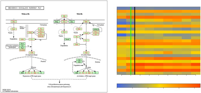
www.nature.com/scientificreports/                                                                    www.nature.com/scientificreports

                                Figure 1. Overview of existing approaches as categorized by looking at the time component (horizontal axis)
                                and the system information (vertical axis). From the time component perspective one can distinguish between
                                two categories: snapshot data and time course data. Time course data is richer in information but also has
                                increased complexity as opposed to snapshot data. From the system information perspective one could consider
                                sets of genes together with their interactions (pathways) or without such interactions (gene sets). Pathways
                                are much richer in information but also have increased complexity as opposed to gene sets. Based on these
                                categories, the existing methods can be divided into the four groups shown, of which the gene set analysis is
                                the most common, including more than 70 methods64,65. Gene set analysis takes as input a collection of gene
                                sets and a snapshot of expression data that compares two phenotypes and ranks the gene sets based on their
                                relevance to the phenotype computed by the analysis. Pathway analysis has the same workflow as the gene set
                                analysis but also takes into consideration the interactions between the genes as described by the topology of the
                                pathways66,67. Network discovery from time course data takes as input data collected at multiple time points and
                                a set of genes and infers relations between the genes in the input set68. Network dynamic analysis is the most
                                recent, and has only 4 existing methods10–12,69. Methods in this category (including the proposed method) use
                                time series data and pathways to gain knew knowledge about the underlying phenomena.

                                    In practical terms, the data to be analyzed is a time series of gene expression or any other sequential meas-
                                urements of systemic states such as the one described in disease progression. Time-series data have been used in
                                many ways, e.g. to infer information regarding regulatory mechanisms, the rate of change for a gene, the order in
                                which genes are (de)activated, and the causal effects of gene expression changes3. Often, time series-data are used
                                to extract gene profiles that can be be used to better understand the phenomena or phenotypes4–7. The analysis
                                of time-series data can also be used to identify disease biomarkers either as a single gene, a group of genes, or a
                                network of genes8.
                                    In the landscape of analysis methods for high-throughput data (see Fig. 1), the proposed method falls under
                                the category of dynamic network analysis. Other methods in the same category aim to either identify significantly
                                perturbed systems9, time intervals with the highest difference in expression for each gene from a predefined set10,
                                dynamic network biomarkers using local network entropy11, or time periods of differential gene expression using
                                Gaussian processes12. However, all of these approaches perform comparisons between disease profiles and a refer-
                                ence profile (e.g. healthy). In the paradigm proposed here, none of these existing methods can be applied because
                                the goal is to identify a transition to a qualitatively different state without knowing the gene expression profile of
                                the new state, and hence, without the ability to make a comparison between the control and disease phenotypes.
                                    A biological system is characterized by a tendency to reach and maintain a state of homeostatic balance,
                                considered to be a stable state. An alteration made by internal or external stimuli can trigger the system to tran-
                                sition from one stable state to another, referred to as a qualitative change. Notably, any of the system components
                                taken in isolation may not vary dramatically; however, the system as a whole may undergo a qualitative change.
                                Conversely, in a resilient system, important variations of one or a group of components may happen without nec-
                                essarily involving a qualitative systemic change. Importantly, most systems have built-in tolerance mechanisms

Scientific Reports | (2020) 10:8146 | https://doi.org/10.1038/s41598-020-62578-8                                                                    2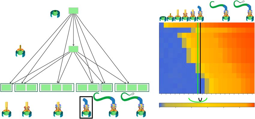
www.nature.com/scientificreports/                                                                    www.nature.com/scientificreports

                                such that the response to a stimulus is delayed until the signal is perceived as real in order to filter noise and to
                                conserve the energy necessary to undergo a systemic change.
                                    We developed and implemented a data analysis method capable of detecting qualitative changes in biological
                                systems despite these challenges. The workflow of the analysis is summarized in Fig. 2. The input to QCD consists
                                of: (i) time-series data and (ii) a network model of the biological system under study. QCD uses the input data to
                                evaluate the system perturbation between each pair of time points/system states using a pathway impact analysis
                                approach13–16. An expectation maximization algorithm is then used to separate large and small system pertur-
                                bations values, thus identifying important differences between those states. Lastly, the analysis finds the disjunct
                                overlaps of the intervals with large system perturbation that identify one or more time intervals during which the
                                biological systems has undergone qualitative changes, referred to henceforth as change intervals.

                                Results
                                Conventional approaches to the analysis of time series gene expression data are extremely useful tools to identify
                                genes that are behaving in a similar way. However, these methods are not designed to identify systemic changes.
                                The goal of the proposed approach is to identify transitions from one state to another, rather than study a par-
                                ticular state or a particular time profile. Our goal is to show that the proposed approach is able to identify such
                                meaningful transitions across different organisms and various phenomena.
                                    The analysis of eight well-studied phenomena was performed with the proposed method (QCD) for seven
                                model organisms using both synthetic and real data. To assess the ability of QCD to detect qualitative changes,
                                results were compared to prior knowledge of the phenomenon under study. QCD uses system knowledge, as
                                described by a known gene signaling network or a map of neurons and their synaptic connections, as well as
                                sequential measurements of the system components (genes or neurons). Data were obtained by measuring either
                                the mRNA level of the genes involved in the system, in the case of real data, or generated based on equations
                                describing the model of each organism, in the case of synthetic data.
                                    The results of the analyses show that QCD can reliably identify the time interval during which a biological
                                system goes from one qualitative state to another in response to organism development or to a shift in environ-
                                mental conditions. We evaluate the method using phenomena that involve major physiological changes. We also
                                evaluate the method for phenomena involving more subtle, yet important changes. Major physiological changes
                                analyzed using synthetic data are E. coli flagellum building17,18 and B. subtilis sporulation17,19. The subtle change
                                analyzed using synthetic data is C. elegans avoidance reflex17,20. Major physiological changes analyzed using real
                                gene expression data are yeast sporulation21 and fruit fly pupariation22. More subtle changes analyzed using real
                                gene expression data involve fruit fly ethanol exposure23.
                                    QCD was compared with an existing method developed by Liu and colleagues used to detect network bio-
                                markers and the pre-disease state (herein abbreviated DNBM)11. In addition to the six datasets mentioned above,
                                we also ran QCD on the two datasets from the Liu et al. study. The first dataset is derived from a mouse study of
                                exposure to a toxic gas (carbonyl chloride). Using these data QCD identified one qualitative change, before the
                                exposure became lethal, preceding the pre-disease state detected by Liu et al. The second dataset contains data
                                describing the progression of human hepatocellular carcinoma. Using these data, QCD identified a qualitative
                                change from a benign stage (control) to a pre-malignant stage (high-grade dysplastic nodules), also preceding the
                                pre-disease state detected by the Liu et al. study.

                                Bacterium flagellum building.              When in an environment lacking nutrients, the E. coli bacterium initiates
                                the process of building a flagellum that will provide the motility necessary for finding an environment rich in
                                nutrients.
                                     We analyzed the process of building the E. coli flagellar motor, using synthetic data and the flagellum building
                                network18 (see Fig. 3A). Previous studies describe this network as a multi-output coherent type 1 feed-forward
                                loop (C1-FFL)18,24. A C1-FFL is a network in which one gene activates another and, together, they activate another
                                gene or (groups of) genes in the multi-output networks24,25.
                                     The flagella building network is a generalization of the C1-FFL. In essence, the flagella building network is a
                                multi-output C1-FFL in which the exact timing of the sequence of steps is controlled by the different activation
                                thresholds (see the edge labels in Fig. 3A). These thresholds ensure that all the elements of the flagellum are built
                                in a specific order so that it can properly assemble (e.g. the base of the structure must be in place before all other
                                elements). Due to the different activation thresholds, a reverse order of the activation thresholds for flhDC and
                                 fliA yields a first-in first-out (FIFO) order in the gene transcription. This is typical of sensory transcription net-
                                works as a mechanism used to filter out (not react to) noise containing false positive signals of short duration.
                                     Gene expression data was generated for the flagellum building network for a period of 10 hours using a con-
                                tinuous function that models the protein accumulation and parameters from previous studies17,18. Samples were
                                taken every 30 minutes leading to a gene expression time course dataset with 21 time points. Panel B in Fig. 3
                                shows the evolution of gene expression over time for the genes involved in this phenomenon.
                                     Importantly, the organism commits to building the flagellum when the first hook of the flagellar motor starts
                                to be built ( fliA reaches the threshold to regulate the next group of genes, fliD and flgK )18. This is an important
                                check point in the flagella building process as the assembly of the following component can still be halted if nec-
                                essary26. However, after this checkpoint, the bacterium commits to building the flagellum (see the top of panel B
                                in Fig. 3). For these reasons, the interval between 240 and 270 minutes can be considered the boundary that
                                separates the two qualitatively different states: with and without flagellum. The goal of our approach is to find this
                                interval without any knowledge about the phenomenon and with knowledge only from the gene expression data
                                and the network of the system.

Scientific Reports | (2020) 10:8146 | https://doi.org/10.1038/s41598-020-62578-8                                                                     3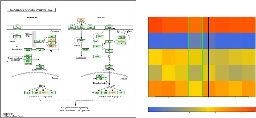
www.nature.com/scientificreports/                                                                  www.nature.com/scientificreports

                                Figure 2. Workflow of the QCD method. The algorithm takes as input time series data and network(s) that
                                models the biological system. The time series data is used to compare every pair of time points (time interval).
                                In STEP I, a pathway impact analysis is used to compute a perturbation score for each comparison. In STEP
                                II, an expectation maximization algorithm is employed to identify the parameters of a gamma mixture model
                                and select the interval(s) when the system/pathway/network experienced a large perturbation. In STEP III,
                                change intervals are selected by identifying the overlap of the set of intervals with large system perturbation and
                                selecting the narrowest disjunct time intervals.

Scientific Reports | (2020) 10:8146 | https://doi.org/10.1038/s41598-020-62578-8                                                                  4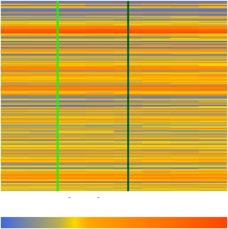
www.nature.com/scientificreports/                                                                     www.nature.com/scientificreports

                                Figure 3. The input and results of the qualitative change detector (QCD) for the E. coli flagella building
                                phenomenon. Panel (A) The multi-output coherent type 1 feed-forward loop (C1-FFL) network that describes
                                the flagellum building, together with the activation thresholds (β on the edge) for each of the six groups of genes
                                (dark green boxes)17,18. The flagellum building is depicted in the cartoons matching the activation of each group
                                of genes. The black box denotes building the flagellum hook which is the point of no return in this process and
                                hence the real change interval that we aim to discover. Panel (B) The heatmap of the sampled data (input to
                                QCD), and the real change interval (black arc below the heatmap and black vertical line positioned in the center
                                of the interval) as described by literature. The change interval detected by QCD is shown by the green arc below
                                the heatmap and the green vertical line positioned in the center of the interval (very close to the black line
                                showing the actual point of no return). The stages of the flagella building are presented as cartoons in
                                chronological order on the top part of the figure.

                                    The E. coli flagellum construction is controlled by two transcription factors, flhDC and fliA (see Fig. 3A). The
                                master regulator flhDC activates fliA and there is an OR relationship through which these two master regulators
                                activate the other genes in the network (12 genes). The genes are part of 6 groups: (i) fliL, (ii) fliE and fliF , (iii)
                                 flgA, flgB, flhB, (iv) fliD, flgK , (v) fliC , (vi) meche, mocha and flgM .
                                    QCD compares all system states (time points) to each other using a pathway impact analysis. In essence, the
                                state of the system at each time point is compared to the state at all other time points using a pathway impact
                                analysis13 that takes into consideration all gene expression changes, the position of each gene on the pathway
                                (Fig. 3A), and the type and direction of every interaction to determine if the state of the system was altered. The
                                result of this impact analysis is a set of system perturbation factors that quantify the system perturbation. To
                                determine the significant system perturbations, we assume there are two types of intervals: i) those with large
                                perturbations between the states involved, and ii) those with small perturbations caused only by random fluctua-
                                tions. We then use an expectation maximization algorithm to fit a gamma mixture model of two distributions to
                                the perturbation factors (see Fig. 4). The intersection of the two distributions will be the optimal threshold that
                                can be used to separate the large perturbations from the small perturbations as presented in Fig. 4A. Using this
                                approach, we assign a “large” or “small” perturbation status to each comparison. Panel B in Fig. 4 shows all the
                                state comparisons considered, in which the gray and black arcs show small perturbations and the red arcs show
                                large perturbations between the states of the system at those time points.
                                    In essence, most of the comparisons between any time point earlier than 180 mins and any time point after 300
                                mins show large perturbations (exceptions are marked by the black arcs). This suggests that a qualitative change
                                of the system occurs between 180 and 300 mins, which is indeed the case. The real change takes place between 240
                                minutes, when fliD and flgK expression begins, and 270 minutes, when fliA starts to regulate the next group of
                                genes and the building of the first hook of the flagellar motor begins.
                                    The identification of a change interval should be followed by an analysis of the states of the system before and
                                after a change interval in order to gain insight into the system transition. Without loss of generality, we will con-
                                sider the situation in which there is a single change interval, as in this dataset. Furthermore, we also assume that
                                the system is in a stable state before and after the change interval. Under these circumstances, we can group the
                                states in which the system is stable into meta-states.
                                    A meta-state is a group of consecutive states where all comparisons between states within a meta-state have a
                                small perturbation and all comparisons between states from a meta-state to states outside it (excluding the states
                                in any change intervals) have a large perturbation.
                                    The results shown in panel B of Fig. 4 suggest that states S0–S6 might form a meta-state, MS1. Similarly, the
                                states S10–S20 might define a second meta-state, MS2. To investigate these potential meta-states, all comparisons
                                (arcs) were studied from the perspective of the above definition of a meta-state. From this perspective, all these
                                comparisons can be either consistent or inconsistent with the expectations noted above. This is a binary choice,
                                and under the null hypothesis in which there are no meta-states, the probability that a comparison is consistent
                                or not should be 0.5. Based on this framework, a binomial model can be used to calculate a p-value characterizing

Scientific Reports | (2020) 10:8146 | https://doi.org/10.1038/s41598-020-62578-8                                                                      5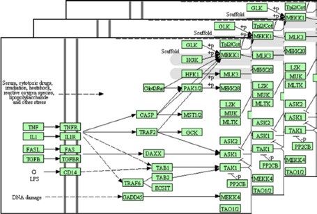
www.nature.com/scientificreports/                                                                   www.nature.com/scientificreports

                                Figure 4. Identifying the qualitative change interval for the E. coli flagella building phenomenon. Panel (A)
                                Identifying state comparisons involving large perturbations. The black line shows the observed density of
                                the perturbation values for all pairwise comparisons of system states. We assume that some comparisons
                                will be characterized by large perturbations, while others by small perturbations. A mixture of two gamma
                                distributions are fitted to the observed data to yield the distributions of large (red) and small (blue) perturbation
                                whose mixture best fits the observed data (red and blue lines). The intersection point (yellow vertical line) is
                                the optimal threshold used to distinguish between the large and small perturbations. Panel (B) The arcplot of
                                all comparisons performed by QCD between all pairs of system states. Red arcs, above the x axis, represent
                                comparisons that show a large perturbation, while gray arcs, below the x axis, represent comparisons with a
                                small perturbation. All the comparisons between states in the intervals S0–S6 and S10–S20 are associated with
                                small perturbations. At the same time, the vast majority of all possible comparisons between any state in the
                                interval S0–S6 and any state in the interval S10–S20 are associated with large perturbations. The black arcs
                                are comparisons between a state in the interval S0–S6 and a state in the interval S10–S20 that are associated
                                with small system perturbations. The smallest interval of overlapping large perturbation intervals, the interval
                                between S6 and S10, is the detected change interval.

                                the amount of evidence that indicates the existence of a true meta-state (comparisons consistent with the defini-
                                tion vs. inconsistent comparisons). More details can be found in the Methods section, subsection “Meta-states
                                statistical validation”. Groups of states with significant p-values will be reported as meta-states.
                                    In this case, both groups of states identified by QCD had highly significant p-values: p = 5.44 × 10⁻¹⁹ for
                                meta-state 1 (S0–S6) and p = 3.61 × 10⁻²⁸ for meta-state 2 (S10–S20).

                                Bacterium sporulation. When deprived of food, the B. subtilis bacterium turns into a spore, a robust struc-
                                ture able to survive in an environment lacking nutrients. This is a crucial feature that ensures the bacterium’s
                                survival in an environment scarce in food in which it cannot survive in its active form.
                                    Compared to the E. coli flagellum-building network, which includes only activation signals, the network con-
                                trolling sporulation also includes repression signals (Fig. 5A). This network has a hierarchical structure that
                                consists of four transcription factors: sigmaE , sigmaK , GerE , SpoIIID and three groups of genes Z1, Z2, Z3. This
                                network is comprised of two network motifs, each of them represented by two networks. The two coherent
                                feed-forward loops (C1-FFLs) aim at sigmaK and Z3, respectively, while the two incoherent type-1 feed-forward
                                loops (I1-FFLs) are centered around Z1 and Z2, respectively. The C1-FFLs are denoted as coherent because their
                                central genes, sigmaK and Z3, respectively, receive activation signals from both genes upstream of each.
                                Specifically, sigmaK receives activation signals from both SpoIIID and sigmaE , while Z3 receives activation signals
                                from both GerE and sigmaK . In contrast, the incoherent network is characterized by a gene that receives one acti-
                                vation and one repression signal from the two genes immediately upstream of the target gene. For example, Z1 is
                                activated by sigmaE but repressed by SpoIIID.
                                    The gene expression data was sampled from the spore formation network for a period of 10 hours using a
                                continuous function that models the protein accumulation and parameters observed in previous studies17,19.
                                Samples were taken every 30 minutes leading to a gene expression time course dataset with 21 time points.
                                    Importantly, the organism commits to the spore formation when the second suppressor (GerE ) is expressed (4
                                h = 240 min)19. In turn, GerE is regulated by sigmaK which also regulates the communication between the mother
                                cell and the spore through a checkpoint that is crucial for the formation of viable spores. Hence, the true interval
                                of change is the interval between 210 minutes, when sigmaK shows the first change in expression, and 240 min-
                                utes, when GerE shows the first change in expression.
                                    Our method was applied on the sporulation network and the synthetic gene expression dataset obtained by
                                the above sampling. In these data, QCD identified one change interval (210–240 min) (Fig. 5B). The detected
                                interval exactly matches the time interval between the time when the spore formation starts (GerE is being
                                expressed) and up to the moment when the next group of sporulation genes (Z2) is activated.
                                    We also evaluated the two groups of system states: before the change interval (0–210 min) and after the change
                                interval (240–600 min), as potential meta-states MS1 and MS2, respectively. The p-value for each was highly
                                significant: p = 2.31 × 10⁻¹⁹, for MS1, and p = 6.23 × 10⁻³², for MS2. These p-values validate the hypothesis
                                that these are true meta-states. Interestingly, these meta-states can be mapped to the rod-shaped bacterium form
                                and the endospore form, respectively, while the detected change interval can be associated with the process of

Scientific Reports | (2020) 10:8146 | https://doi.org/10.1038/s41598-020-62578-8                                                                   6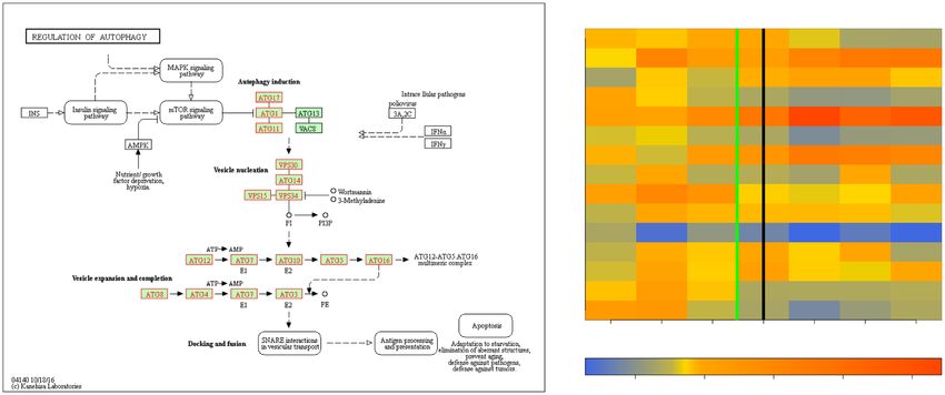
www.nature.com/scientificreports/                                                                    www.nature.com/scientificreports

                                Figure 5. The input and results for QCD for B. subtilis sporulation. Panel (A) shows the sporulation network.
                                The genetic network represented by the two coherent type 1 feed-forward loops (C1-FFLs) and two incoherent
                                type-1 FFLs (I1-FFLs) that describe the sporulation network as reported in previous studies17,19. Panel (B)
                                shows the heatmap of the sampled data. The real change interval is shown by the black arc below the heatmap
                                (black vertical line positioned at the average of the interval limits) as described by literature. The change interval
                                detected by the proposed method is shown by the green arc (green vertical lines positioned at the average of the
                                interval limits), match perfectly with the actual timing of these events.

                                spore formation. These results are consistent with previous studies and interpretations19. Specifically, the sigmaK
                                factor expression was identified as the critical control element in the regulatory mechanisms and the coordination
                                of spore formation between the mother cell and forespore. In particular, sigmaK activates GerE which in turn
                                triggers the expression of the last set on genes. For this reason, the true time point that can be considered as sep-
                                arating the rod-shaped bacterium from the endospore state is the point in which sigmaK becomes expressed
                                (shown by the black line in Fig. 5). Before the change interval, the bacterium preserved most of its initial charac-
                                teristics, while after this interval, the bacterium assumed most of the characteristics of an endospore. During the
                                change interval, the system exhibited characteristics of both “spore” and “no spore” states. To conclude, in the
                                study of Bacterium sporulation phenomenon, DQC accurately identified the transition from the rod-shaped
                                bacterium form (no spore) to the endospore (spore) form.

                                Worm avoidance reflex.                A phenomenon involving more subtle changes is the nociception reflex.
                                Nociception is a sensory process that allows the detection of harmful stimuli and activates a reflex response to
                                move a part of the body or the whole body away from the stimulus. Nociceptors are present in fish, worms, and
                                fruit flies, among others, and help trigger an avoidance reflex such as a backward movement. In the roundworm
                                (C. elegans), the avoidance reflex network is composed of two parallel receptor neurons that communicate with
                                two sequential command neurons (Fig. 6A).
                                    The C. elegans avoidance reflex network is a generalization of the C1-FFL in the form of a multi-input C1-FFL.
                                As previously described, C1-FFL is a network of three nodes in which one node activates another and, together,
                                they activate another node24,25. In multi-input C1-FFL networks, the initial activation is performed by multiple
                                nodes or groups of nodes rather than by just one node. ASH is the main nociceptor and triggers avoidance behav-
                                ior in response to harmful stimuli such as the nose touch and volatile chemicals. FLP is a sensory neuron trig-
                                gered by painful, heat-related stimuli or mechanical stimuli, such as a harsh nose touch, that initiates the
                                nematode’s backward movement. AVD is a command interneuron that functions as a modulator for backward
                                locomotion induced by a head touch. Neurons AVA and AVD drive the worm’s backward movement.
                                    Neuronal signal data was generated for the avoidance reflex network over a period of 8 milliseconds, using a
                                continuous function that models the signal processing and parameters observed in previous studies17,20. Samples
                                were taken every millisecond leading to a time course dataset with eight time points.
                                    The nematode commits to the backward movement at 3ms, which is the moment the nose touch (FLP - spik-
                                ing function) reaches the threshold to trigger the second command interneuron ( AVD). The movement starts at
                                5ms when the AVA neuron starts firing20. The two time-points mark the 3 to 5 ms time interval which is the real
                                change interval. Using these data, QCD identified the narrower 4 ms to 5 ms interval (Fig. 6B).
                                    In addition, the two groups of system states, before and after the change interval, were evaluated as potential
                                meta-states. The p-values for the two groups of states are highly significant: p = 4.28 × 10⁻⁴ for meta-state 1 and
                                p = 4.28 × 10⁻⁴ for meta-state 2. In summary, in the case of the avoidance reflex, the detected change interval is
                                a transition between “no movement” and “moving backward” meta-states.
                                    Results of the first three case studies, for which we used synthetic data, proved that QCD can be quite accurate.
                                However, in practice, the data from real biological experiments can be very noisy. In order to investigate the capa-
                                bilities of this approach to detect the correct change interval from real gene expression data, we used datasets col-
                                lected from three different experiments: yeast sporulation, fruit fly metamorphosis, and acute ethanol exposure

Scientific Reports | (2020) 10:8146 | https://doi.org/10.1038/s41598-020-62578-8                                                                     7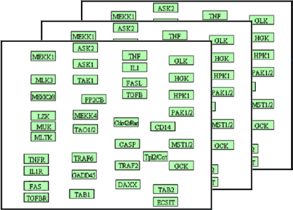
www.nature.com/scientificreports/                                                                   www.nature.com/scientificreports

                                Figure 6. The input and results for QCD for the C. elegans avoidance reflex. Panel (A) top: The network that
                                describes the avoidance reflex network as presented in previous studies17,20 is a multi-input coherent type 1 feed-
                                forward loop (C1-FFL) with two inputs. Synaptic weights are marked by the β values on the edges. Panel (A)
                                bottom: The signal dynamics of the avoidance reflex network. Panel (B) The heatmap of the sampled data
                                (which is the input to QCD) and the real change interval shown here by the black arc below the heatmap (black
                                vertical line positioned in the center of the interval) as described by literature. The change interval detected by
                                the proposed method and shown by a green arc below the heatmap (vertical lines positioned in the center of the
                                interval), matches almost perfectly with the actual timing of these events.

                                (see Figs. 7, 8 and 9). All data are available in the public domain in the Gene Expression Omnibus (GEO)27,28.
                                Again, we chose different phenomena and different model organisms for a thorough method evaluation.

                                Baker’s yeast sporulation.            Starvation for nitrogen and carbon sources (high stress) induces meiosis and
                                spore formation in diploid yeast (S. cerevisiae) cells. Stress-tolerant haploid spores are formed through cell divi-
                                sion (meiosis) within the mother cell. This is a qualitative and obvious physiological change in yeast cells adapt-
                                ing to their environment. The sporulation process has been thoroughly studied and is well understood21, which
                                makes it a good candidate on which to validate QCD.
                                   We used the Kyoto Encyclopedia of Genes and Genomes (KEGG)29–31 pathway database as a source for
                                the biological networks describing the studied phenomena. The regulation of autophagy pathway (KEGG ID:
                                sce04140) describes the phenomena involved in sporulation. This pathway consists of mechanisms involved in
                                processing internal and external stresses including nutrient availability. As a result, regulation of autophagy is
                                essential for survival because it is used to maintain important cellular functions when environmental conditions
                                change.
                                   The QCD method was applied on the regulation of autophagy pathway and gene expression data from the
                                yeast sporulation study by Chu et al. (GSE27,21). Panel A in Fig. 7 shows this pathway, as well as the genes meas-
                                ured in this experiment, marked in red. The experiment spanned 11.5 hours and data were collected at seven une-
                                qually spaced time points (0, 0.5, 2, 5, 7, 9, and 11.5 hours). The experiment was designed such that the sampling
                                captures all known stages of the biological process. Sporulation is divided into four major stages: early, middle,
                                mid-late, and late21.
                                   The commitment to sporulation starts in the middle stage (2–5 h) and spans the mid-late stage (meiosis II
                                phase, 5–7 h)21. Therefore, the true change interval for this phenomenon is 2 h to 7 h. As observed by Chu et al.,
                                the transition phase ends after the mid-late stage. This study also showed that one of the first discernible steps of
                                spore morphogenesis occurs after the meiosis II spindles are formed, which makes the late phase a stable one.
                                Also, the middle-late phase is still part of the change interval as previous studies reported that the middle-late
                                phase includes the major cytological events of sporulation32,33. Panel B of Fig. 7 displays the measured changes of
                                the genes on the regulation of autophagy pathway over the time course noted above.
                                   In this case, QCD identifies a qualitative change in the interval from 0.5 h to 7 h, which includes the real
                                change interval (2 h to 7 h) and starts one time point earlier. The change interval is the transition that separates
                                the two potential meta-states (active state and spore state). The active and spore potential meta-states have
                                p-values of p = 0.062 and p = 0.0195, respectively.
                                   Sometimes small gene-level changes (not noticeable by eye) across the system can lead to important systemic
                                changes. This is exactly the problem that our method was designed to address: the inability to easily identify
                                important qualitative changes when they happen incrementally. The transition from healthy to disease is in many

Scientific Reports | (2020) 10:8146 | https://doi.org/10.1038/s41598-020-62578-8                                                                   8
www.nature.com/scientificreports/ www.nature.com/scientificreports
Figure 7. The input and results for QCD for yeast sporulation. The input is the regulation of autophagy
pathway from KEGG29– 31 (sce04140)*, in Panel (A), and gene expression data from the GEO dataset GSE27, in
Panel (B). The data captures the sporulation phenomenon, specifically the transition from diploid cells through
meiosis to the spore cells. Panel (B) shows the heatmap of the time course (0 to 11.5 hours) for the measured
KEGG pathway genes (in red), with the change interval detected for the phenomenon (green arc and the green
vertical line in the center of the interval (0.5–7 h)), as well as the real change interval (black arc and the black
vertical line in the center of the interval (2–7 h)). *For details about the pathway notations see the KEGG legend
at: https://www.genome.jp/kegg/document/help_pathway.html.
Figure 8. The input and results for QCD on fruit fly metamorphosis (pupariation). The input is the Hedgehog
pathway from KEGG29– 31 (dme04340), in Panel (A), and gene expression data from the GEO dataset GSE3057,
in Panel (B). The data captures the pupariation phenomenon, specifically transition from the end of the larva
stage through the prepupa stage and to the beginning of the pupa stage of the fruit fly. Panel (B) shows the
heatmap of the time course (−18 to 12 hours) for the measured KEGG pathway genes (in red), with the change
interval detected for the phenomenon (green arc and the green vertical line in the center of the interval (−18–0
h)), as well as the real change interval (black arc and the black vertical line in the center of the interval (−4–0
h)).
cases similar to the transition from young to old: any two consecutive measurements taken at short intervals are
unlikely to show any important changes. However, the transition is happening and at some point, the current state
will be significantly different from states long before. Our method is designed precisely for the purpose of detect-
ing such changes and distinguishing them from mere random fluctuations present in any stable state.
Scientific Reports | (2020) 10:8146 | https://doi.org/10.1038/s41598-020-62578-8 9www.nature.com/scientificreports/ www.nature.com/scientificreports
Figure 9. The input and results for QCD on fruit fly ethanol exposure. The input is the Hedgehog pathway from
KEGG29– 31 (dme04340) in Panel (A), and gene expression data from GEO GSE18208, in Panel (B). The data
captures the acute ethanol exposure phenomenon, specifically transition from the “sober” stage through the
“drunk” stage and back to the “sober” stage. Panel (B) shows the heatmap of the time course (control, 0 to 3.5
hours) for the measured KEGG pathway genes (in red), with the change interval detected for the phenomenon
(green arc and the green line in the center of the intervals (0.5–1 h) and (1–1.5 h), as well as the real change
interval (black arc with a black line in the center of the interval (1–2 h)).
Fruit fly metamorphosis. Three major states — egg, larva and pupa — occur during the development of
the fruit fly. The larvae typically pass through three molting stages (instars) during which they shed various body
elements and form new ones. Importantly, the third molting stage the larvae pupate and become adults, which
marks the completion of the metamorphosis process.
The QCD method was applied on the Hedgehog signaling pathway from KEGG29–31 (pathway ID: dme 04340)
and data publicly available for the metamorphosis of D. melanogaster (GSE3057,22). The Hedgehog signaling
pathway, named after the signaling molecule Hedgehog (Hh), has a crucial role in organizing the body plan for
the fruit fly during development. Panel A in Fig. 8 shows this pathway as well as the genes measured in the meta-
morphosis experiment (in red in this figure). The experiment started 18 hours before pupariation, spanned 30
hours, and was sampled at nine time points, two prior to pupariation (−18 hours and −4 hours), and the other
seven time points equally spaced over 12 hours after the actual pupariation (0 h, 2 h, 4 h, 6 h, 8 h, 10 h, 12 h).
Panel B of Fig. 8 shows the measured changes of the genes on this pathway over the time course described
above. Puparium formation is triggered at the end of the third instar larvae stage that occurred during this exper-
iment in the interval from −4 hours to 0 hours, and is marked by a high peak of the steroid hormone
20-hydroxyecdysone22. A second peak of the steroid hormone 20-hydroxyecdysone occurs roughly at the 10-hour
time point and triggers the transformation from prepupa to pupa22. Puparium formation represents the onset of
metamorphosis; therefore, the real change interval for this case study is indeed from −4 hours to 0 hours. The
QCD method identifies one change interval from −18 hours to 0 hours. Notably, the third instar larvae stage,
which starts 24 hours before pupariation and lasts until 0 hours (prepupae phase starts), is not a stable state in
which the organism (fruit fly) exists. Therefore, the QCD not only correctly identifies the qualitative transition
from larva to pupa, but it also shows the organism is in a continuous transition during the third instar larvae
stage. The second change in this experiment (prepupa to pupa) arguably perturbs the system less than the first one
since both prepupa and pupa are part of the pupal stage.
Notably, in this case study the change takes place at the beginning of the time course. To determine
potential-meta-states relative to this change interval, we selected the only state before the change interval (−18 h)
as the potential meta-state 1 and all states after the change interval (0 h–12 h) as potential meta-state 2. These two
meta-states are characterized by highly significant p-values: p = 7.81 × 10⁻³ and p = 3.73 × 10⁻⁹ ,
respectively.
Fruit fly acute ethanol exposure. The fruit fly has been used as a model to study drug addiction. In the
fruit fly, drug addiction produces physiological effects similar to those observed in mammals because the cellular
neuronal mechanism that mediate the signals from the chemical compounds found in these drugs is conserved
across these species.
To apply the QCD method, we used the Hedgehog signaling pathway (KEGG ID: dme04340) and the acute
ethanol exposure data available from GEO (GSE18208) and described by Kong et al.23. The Hedgehog signaling
pathway was chosen for its capability to model major mechanisms involved in fruit fly development, including its
adaptive mechanisms. Panel A in Fig. 9 displays this pathway, as well as the genes measured in this experiment,
Scientific Reports | (2020) 10:8146 | https://doi.org/10.1038/s41598-020-62578-8 10www.nature.com/scientificreports/ www.nature.com/scientificreports
marked in red. Panel B of Fig. 9 shows the measured changes of the genes on this pathway over the time course
from the biological experiment. The experiment spanned 3.5 hours (210 minutes) of recovery after a 30-minute
ethanol exposure, sedating up to 75% of the flies. Samples were taken at eight time points. The time points include
one control, before exposure, one at 0 hour, right after exposure and every 30 minutes after that up to 3.5 hours;
the missing data point at 2.5 hours (150 min) was not provided in the dataset. This experiment’s treatment con-
ditions included exposure to humidified air or ethanol vapor (60%) for 30 minutes, and then recovery for up to
210 minutes23. The recovery period from ethanol sedation has been reported by another study to be approxi-
mately between 40 minutes and 2 hours34, which is the real change interval. Based on this recovery time, by the
end of this experiment (210 minutes), the fruit flies should recover from the effects of ethanol exposure. In the
GSE18208 dataset 40 minutes was not one of the sampled time points; therefore, to mark the real change interval,
we used the very next time point available in the dataset, the one-hour time point.
The intuitive physiological transitions expected for these data are from no exposure (sober) to exposure to
ethanol (drunk) and back to fully recovered (sober). However, the drunken state is temporary, since it is followed
by recovery. Because of this transition, we expected two change intervals, from sober to drunk and from drunk to
sober. Furthermore, the initial and end states (sober before exposure and sober after recovery) were expected to
be very similar from a gene expression point of view. In other words, the sober state is the same in the initial and
final state in this case, as opposed to the flagellum building case where the initial and final states, with and without
flagellum, are obviously different.
The ethanol exposure has a delayed effect at the gene level. According to Kong et al., the expression of immu-
nity genes increased after ethanol exposure in the time range from 0.5 hours to 1.5 hours23. Because of this delayed
effect, we did not expect the biggest changes between the control and 0 hours but rather between the control and
some later time point(s).
The QCD results on these data have shown that the biological system indeed goes through two qualitative
changes, and the change intervals are: 0.5 hours to 1 hour and 1 hour to 1.5 hours, matching the expected transi-
tions from a sober state to a drunken state and then back to the sober state. The effects of the ethanol exposure
appear to peak at the 1-hour time point. Based on the change intervals and the return of the system to its initial
state, there are two groups of states that may form meta-states. These potential meta-states consist of the following
time points: control, 0 hour, 0.5 hours, and 1.5 hours to 3.5 hours, for meta-state 1, and the 1-hour time point for
meta-state 2. The distribution of the significant and non-significant transitions yielded a highly significant
p-value, p = 1.37 × 10⁻⁵, for meta-state 1, but a non-significant p-value ( p = 0.22) for meta-state 2. This result
is probably due to the small number of comparisons involving the single time point included in meta-state 2.
Human hepatitis C virus (HCV) infection to hepatocellular carcinoma (HCC) progression.
Hepatocellular carcinoma (HCC) is a common liver cancer that can be the result of an infection with the hepa-
titis C virus (HCV). The progression from HCV infection spans multiple disease stages before reaching HCC, as
reported by Wurmbach et al.35. We used the data from this study to identify qualitative changes for this phenom-
enon. The dataset (GSE6764,35) contains gene expression collected from 75 samples (48 patients) and covers eight
progressive stages of HCV induced HCC: four no-cancer stages including no HCV/control, cirrhosis, low-grade
dysplastic, and high-grade dysplastic, and four cancer stages including very early HCC, early HCC, advanced
HCC, and very advanced HCC. Normal liver control is used as the initial stage and stages are ordered by disease
progression.
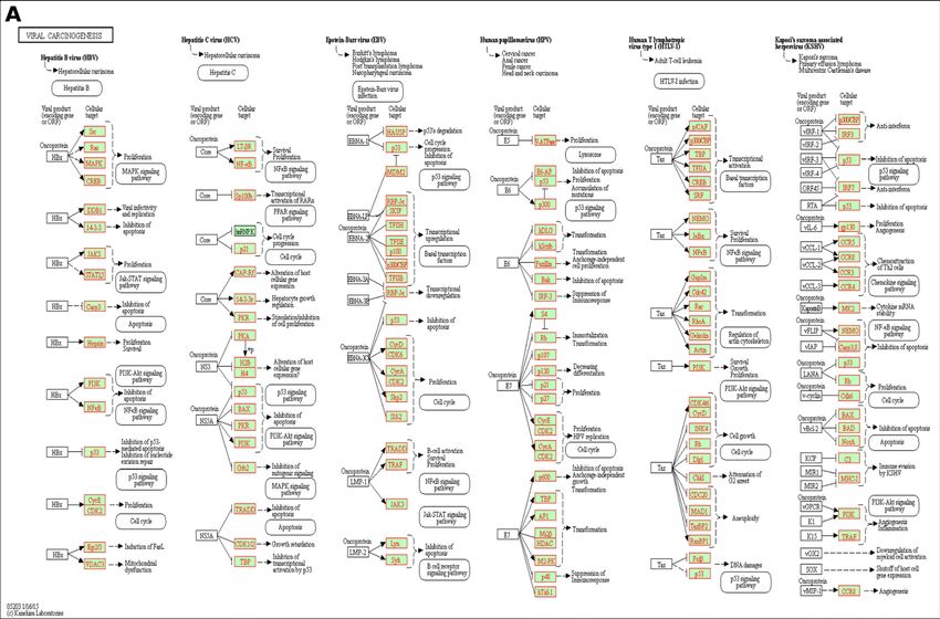
To apply QCD on these data, we used the viral carcinogenesis pathway from KEGG29–31 (hsa05203) as the
network/map of the biological system. The viral carcinogenesis pathway describes the signaling mechanisms
involved in inflammatory responses such as the one triggered by HCV. Panel A in Fig. 10 shows this pathway as
well as the genes measured in this experiment marked in red. Panel B of Fig. 10 shows the measured changes of
the genes on this pathway over the different disease stages from the biological experiment.
From these data, the QCD identified one qualitative change (change interval) from stage zero (control), a
benign state to stage three (high-grade dysplastic), the last of the four benign states and a state in which treat-
ments are effective. The group of states before the change interval was considered as potential meta-state one
(MS1) and contains only the control state. The group of states after the change interval was considered as potential
meta-state two (MS2) and contains five states: high grade dysplastic nodules, very early HCC, early HCC,
advanced HCC, and very advanced HCC. In essence, the analysis identified the transition from the benign state
(first meta-state) to the cancerous state (second meta-state). The p-values of these meta-states were p = 0.031 for
MS1 and p = 3.05 × 10⁻⁵ for MS2.
We compared the results of QCD in this case to the results of an existing method developed to detect net-
work biomarkers and the pre-disease state (DNBM)11. The DNBM takes as input both the high-throughput data
and the large network of protein-protein interactions for the organism under study. The output of DNBM is a
pre-disease state in the form of a sample or list of samples from the data. The hypothesis is that a subset of the
large network, termed the leading network, is the first to change toward the disease state, which makes its compo-
nents and structure causally related with the disease. The DMBM models the change in gene expression over time
as a Markov process. Then, a state-transition-based local network entropy (SNE) is used as a general, early meas-
ure of upcoming transitions by estimating the resilience of the network. The SNE is a Shannon-type entropy36,
intended to quantify the change in state for the biological network.
Notably, the DNBM identifies one single (pre-disease) state prior to the onset of disease, while the proposed
QCD identifies a change interval of transition to disease, which can be much more informative regarding the
disease evolution, as well as providing an opportunity for therapeutic intervention. In addition, in the case of
the QCD, the impact analysis approach may provide a better evaluation of the system’s impact than the network
entropy. At the same time, a reinforcement of the impact by comparing every two time points may provide a
Scientific Reports | (2020) 10:8146 | https://doi.org/10.1038/s41598-020-62578-8 11www.nature.com/scientificreports/ www.nature.com/scientificreports
Figure 10. The input and results for QCD on human hepatitis C virus (HCV) to hepatocellular carcinoma
(HCC) progression. The input is the viral carcinogenesis pathway from KEGG29– 31 (hsa05203), in Panel (A), and
gene expression data from GEO GSE6764, in Panel (B). The data captures the progression from human HCV to
HCC, specifically the transition from control (healthy) through the progressive stages of liver damage up very
advanced HCC. Panel (B) shows the heatmap of the disease progression (control to very advanced HCC) for the
measured KEGG pathway genes (in red), with the change interval detected for the phenomenon (green arc and
the green line in the center of the interval (control – high-grade dysplastic nodules)). The dark green vertical
line (very early HCC) marks the pre-disease state detected by the DNBM method).
better approximation of the change onset. Therefore, evaluating the systemic change between every two time
points results in the early-detection property.
For this case study, the DNBM detected the pre-disease state at the fifth stage, very early HCC, which is the
first malignant stage. The existent DNBM detected the start of the malignant state while our proposed QCD
method detected the transition from benign to malignant.
DNBM was also evaluated on a dataset for mouse exposure to carbonyl chloride (phosgene). Exposure to
carbonyl chloride produces irreversible lung injury and potentially life-threatening pulmonary edema that man-
ifest within a day. We also evaluated the QCD on the same dataset (see Supplementary Methods Section 1.2 for
details). The results in this case yielded perturbation factors that were hard to separate into large and small pertur-
bations resulting in a poor fit of the mixture of gamma distributions. This is indicated by a larger value of the KLD
and smaller value of the KS p-value. For this data set, the KLD yields a value of 2.92 (compared to the other data
sets for which KLD values are around 0.1 or less). Also, the same dataset yields a KS p-value of 0.39. This is still far
from being significant but also very significantly different from all the others which are above 0.85). Even in this
case study, with the worst fit, the QCD method identified one qualitative change which corresponds to the time
interval for the initiation of latent effects of the toxic gas exposure. In other words, QCD identified an interval
during which damage is treatable37, while the DNBM identified a later time point as being the pre-disease state.
These results show the applicability of this method in developing preventive therapies. Identifying the genes
that change within the change interval could lead to the identification of very early markers for disease and poten-
tial targets for disease prevention. A detailed description of the results of the QCD analysis at each step of the
analysis workflow for all eight datasets is included in Section 1 of the Supplementary Methods.
In the case of disease progression, once a change interval is identified one should start the therapeutic inter-
vention as early as possible within the change interval. For example, in the case of the HCV to HCC progression
that could be any time up to the high-grade dysplastic stage.
To further evaluate the potential of the proposed method to detect changes as they occur, we ran the method
on data from only the first three stages of the disease progression. DQC detected a change interval from the first
(control) to the third stage (low-grade dysplastic), showing that a systemic qualitative change is happening and
can be detected at a very early stage, as soon as the disease process has started.
Discussion
Disease prevention and early detection are two major healthcare objectives that contribute to improving quality of
life. Currently, early detection of complex diseases is achieved only after the physiological traits of the phenotype
are present, when existing treatments may be ineffective. Chronic disease, a particular case of complex disease, is
generally detected in the late stage of a relatively slow, progressive process. Representative examples that affect a
large number of people are heart disease, cancer, and neurodegenerative disorders. It is a real challenge for people
with these diseases to maintain a good quality of life after diagnosis. Understanding when the transition to disease
occurs is a good first step towards interrupting the process and maintaining the healthy state.
Scientific Reports | (2020) 10:8146 | https://doi.org/10.1038/s41598-020-62578-8 12www.nature.com/scientificreports/ www.nature.com/scientificreports
To maintain the healthy state, one needs to monitor the biological system and measure the gene expression
or any parameters the system has in order to assess how much the system is changing. The moment a qualitative
change occurs, either cumulative or sudden, a change interval emerges. For instance, in the case of the eight stages
of HCC, a qualitative change occurs from control to high-grade dysplasia. A cirrhotic liver is characterized by
the presence of scar tissue due to long-term damage. In an attempt to replace the damaged cells in the cirrhotic
liver, clusters of newly formed cells can occur in the scar tissue. Dysplastic (abnormally grown) nodules found
in the liver are typically identified in cirrhotic livers. Low-grade dysplastic nodules (LGDN) cells are larger than
the normal liver cells38. High-grade dysplastic nodules (HGDN) cells are smaller than the normal liver cells and
have a greater nucleus-to-cytoplasm-size ratio38. The difference between HGDNs and very early HCC is the stro-
mal invasion present in the latter39. A study on the LGDNs and HGDNs in HCC development concluded that
LGDNs together with large regenerative nodules, should be monitored with ultrasound, while HGDNs should be
preventively treated due to their high malignant risk40. Taken together, these data support the qualitative change
identified by QCD from a low malignant risk stage of the liver disease to a high risk stage and close precursor to
the malignant stage of very early HCC.
To further investigate the results of our analysis in the case of HCC progression, we identified the differentially
expressed (DE) genes (absolute log 2 fold change greater than 1) when comparing the control to high-grade dys-
plasia and the control to very advanced HCC. The total number of measured genes is 20,156. In the control versus
high-grade dysplasia comparison, there are 149 DE genes, while in the control versus very advanced HCC com-
parison, there are 1,355 DE genes, which is almost an order of magnitude higher. This suggests that using the
differentially expressed genes across the change interval, as opposed to the genes that differ between the control
and very advanced HCC, offers a more focused analysis. In essence, the comparison across the narrowest change
interval targets the genes involved in the initial tumor formation, rather than all genes that change as a conse-
quence of the cancer.
The number of common DE genes among the two comparisons is 80, representing 53% of the initial 149 genes.
We downloaded the curated list of cancer genes available in the cancer gene census41 (http://cancer.sanger.ac.uk/
census). This list is presented together with the catalogue of somatic mutations in cancer (COSMIC)42 (http://
cancer.sanger.ac.uk/cosmic). We used this list of cancer genes to filter the 80 common genes to obtain a cancer
gene set. The result consists of two genes: CHEK2 and FAT1 (see Section 2.1 in Supplementary Methods for the
expression profile). These genes are highly relevant to the condition under study considering CHEK2 mutations
have been linked to various cancers43,44; it has also been shown to be a mediator of a tumorigenic mechanism in
HCC45. Furthermore, FAT1 has been shown to have an oncogenic role in HCC46,47, and it has been identified as a
biomarker in multiple cancers48,49.
The viral carcinogenesis pathway from KEGG 29–31 was used to identify the change interval for the
HCV-induced HCC progression. We also used this pathway to filter the 80 common genes and to obtain a “viral
carcinogenesis” gene set, which contains genes from the pathway that change at the onset of the disease. The
result consists of two early growth response genes: EGR2 and EGR3 (see Section 2.2 in Supplementary Methods
for the expression profile). EGR2 has been shown to be an apoptosis promoter gene50, which is downregulated by
miRNAs in cancer51,52. EGR3 has been shown to be involved in a number of cancers and in the regulation of the
immune response53–56, and this gene has recently been linked to HCC when it was used to inhibit the growth of
tumor cells57.
We designed and implemented an analytical method capable of detecting qualitative changes in the state of a
biological system by monitoring its gene expression levels. This has been conducted with no training on previous
examples, with no expert supervision, and with thresholds set using sound statistical criteria. The only hypoth-
esis used here is that a qualitative change will involve enough pathway components to perturb the pathway in a
significant way. The method requires a network of the system, which may limit its applicability. However, most
biological systems do have associated networks. For instance, the KEGG pathway database includes about 200
signaling pathways for human, about 190 signaling pathways for mouse and about 190 signaling pathways for
rat. Many such pathway databases exist: KEGG29–31, Reactome58, BioCarta59, NCI-PID60, WikiPathways61, and
PANTHER62. The proposed method leverages this existing body of knowledge which is expected to grow in the
future. In principle, these diagrams can be used to study how the system changes between states. However, most
or all existing analysis methods would require an a priori definition of the states to be compared. Once these states
are defined, a myriad of methods can be used to identify differentially expressed genes or pathways. One of the
major contributions of the proposed method is that it can detect significant system changes without somebody
having to define them a priori just by monitoring the system.
To evaluate the proposed method, we used both synthetic and real data. The cases used for validation cover
a wide range of biological phenomena and model organisms as presented in the Results section (see Table 1 for
a summary). Identifying a change interval implies recognizing the transition the system goes through from a
state of relative equilibrium to another. The states of relative equilibrium the system transitions from are denoted
here as meta-states and the transition as the change interval. Notably, in each case study, the system transitions
between meta-states that are of great importance if we hypothesize that such transitions are infrequent and that a
qualitative change is required for a system to undergo such transitions. We also assessed the statistical significance
of the potential meta-states for each of the eight case studies. Results show that out of 16 putative meta-states, 13
are significant at a threshold of 5% (see Table 2).
It is important to emphasize that the proposed method accomplishes two goals. First, the method identifies
qualitative changes. These changes are identified based on the system perturbation factors. Second the meth-
ods also identifies meta-states, if they exist. A meta-state is a group of states that are very similar to each other.
Sometimes, qualitative changes happen between meta-states and sometime qualitative changes happen without
clear meta-states on both sides of the change. The p-values in Table 2 are used to test the hypothesis that a group
Scientific Reports | (2020) 10:8146 | https://doi.org/10.1038/s41598-020-62578-8 13You can also read