How Vulnerable Are American States to Wildfires? A Livelihood Vulnerability Assessment - MDPI
←
→
Page content transcription
If your browser does not render page correctly, please read the page content below
fire

Article
How Vulnerable Are American States to Wildfires?
A Livelihood Vulnerability Assessment
Janine A. Baijnath-Rodino * , Mukesh Kumar                         , Margarita Rivera, Khoa D. Tran             and Tirtha Banerjee

                                          Department of Civil and Environmental Engineering, University of California, Irvine, CA 92697, USA;
                                          mukeshk@uci.edu (M.K.); margar5@uci.edu (M.R.); khoadt3@uci.edu (K.D.T.); tirthab@uci.edu (T.B.)
                                          * Correspondence: jbaijnat@uci.edu

                                          Abstract: Quantifying livelihood vulnerability to wildland fires in the United States is challenging
                                          because of the need to systematically integrate multidimensional variables into its analysis. We
                                          aim to measure wildfire threats amongst humans and their physical and social environment by
                                          developing a framework to calculate the livelihood vulnerability index (LVI) for the top 14 American
                                          states most recently exposed to wildfires. The LVI is computed by assessing each state’s contributing
                                          factors (exposure, sensitivity, and adaptive capacity) to wildfire events. These contributing factors
                                          are determined through a set of indicator variables that are categorized into corresponding groups
                                          to produce an LVI framework. The framework is validated by performing a principal component
                                          analysis (PCA), ensuring that each selected indicator variable corresponds to the correct contributing
                                factor. Our results indicate that Arizona and New Mexico experience the greatest livelihood vulnera-

                                          bility. In contrast, California, Florida, and Texas experience the least livelihood vulnerability. While
Citation: Baijnath-Rodino, J.A.;          California has one of the highest exposures and sensitivity to wildfires, results indicate that it has a
Kumar, M.; Rivera, M.; Tran, K.D.;        relatively high adaptive capacity, in comparison to the other states, suggesting it has measures in
Banerjee, T. How Vulnerable Are           place to withstand these vulnerabilities. These results are critical to wildfire managers, government,
American States to Wildfires?
                                          policymakers, and research scientists for identifying and providing better resiliency and adaptation
A Livelihood Vulnerability
                                          measures to support states that are most vulnerable to wildfires.
Assessment. Fire 2021, 4, 54.
https://doi.org/
                                          Keywords: wildfire; livelihood vulnerability index; sensitivity; adaptive capacity; exposure
10.3390/fire4030054

Academic Editors: Fantina Tedim,
Vittorio Leone and
Carmen Vázquez-Varela                     1. Introduction
                                                Wildfires are crucial for ecosystem dynamics by balancing fuel types and creating
Received: 25 June 2021                    appropriate vegetation for maintaining healthy forested regimes [1]. Despite the integral
Accepted: 21 August 2021                  ecological role of wildfires, uncontrolled burns can cause widespread environmental,
Published: 27 August 2021                 economic, social and sustainable development impacts [2–4]. Such wildfire impacts include
                                          losses to human lives; incurring financial losses from buildings and homes; widespread
Publisher’s Note: MDPI stays neutral      social, health and economic costs through evacuations, smoke exposure, and loss of tourism
with regard to jurisdictional claims in   revenue [5–7]. The Insurance Information Institute, gives an example of financial loss due
published maps and institutional affil-   to wildfires, including the 2019 wildfires in California and Alaska that created a loss of
iations.
                                          4.5 billion dollars in damages, largely resulting from the California Kincade and Saddle
                                          Ridge wildfires. In order to minimize ignition and spread during this time, California’s
                                          electrical utility provider issued rolling blackouts to homes and businesses during high
                                          wind and extreme dry conditions. However, this inevitably cost the state billions of
Copyright: © 2021 by the authors.         dollars in losses [8]. It is therefore evident that wildfires have a direct impact on the
Licensee MDPI, Basel, Switzerland.        livelihood of many residents in fire-prone communities within the United States, making
This article is an open access article    them vulnerable to wildland fire exposure [9].
distributed under the terms and                 Besides economic impacts, changes in social and climate conditions can significantly
conditions of the Creative Commons
                                          affect fire regimes, producing greater potential damage than those previously thought [2].
Attribution (CC BY) license (https://
                                          Social factors, such as the expansion of the wildland–urban interface (WUI) (where human
creativecommons.org/licenses/by/
                                          settlements, buildings, and wildland vegetation meet), have influenced the dramatic
4.0/).

Fire 2021, 4, 54. https://doi.org/10.3390/fire4030054                                                           https://www.mdpi.com/journal/fire
Fire 2021, 4, 54                                                                                             2 of 29

                   increase in wildfire suppression costs, as well as the number of homes lost to wildfires in the
                   United States (US) over the past 30 years [7,10,11]. The 2019 wildfire risk report shows that
                   the US experienced the sixth-highest acres burned in 2018 since the mid-1900s. According
                   to the National Interagency Fire Center (NIFC) report, California has topped the list in the
                   US with over 1.8 million acres burned in 2018 [12]. Climate factors such as extreme weather
                   conditions can also influence the escape of wildland fires during suppression practices,
                   leading to unplanned destructive fire behavior [7,13], thereby worsening environmental
                   and socio-economic impacts.
                         There have been many wildfire risk assessment studies that use a wide range of wild-
                   fire danger indices [14]. However, many of these indices focus mainly on specific hazard
                   components of wildfires (behavior, danger, threat) and consider biophysical components of
                   weather conditions, topography, fuel, fire size, rate of spread, suppression difficulty, fire
                   occurrence, or burn severity to generate fire risk assessment maps [15]. Studies, such as
                   that of [16], have evaluated fire risk on structures, taking into account variables pertaining
                   to topography, spatial arrangement, and vegetation. However, meteorological factors
                   (atmosphere and weather patterns), building materials, and fire suppression efforts within
                   different fire regions are also important to consider. It is acknowledged that combining
                   these various multidimensional socio-economic and biophysical variables into a risk and
                   vulnerability assessment framework can be challenging. While various studies have at-
                   tempted to bridge the gaps among the social, natural, and physical sciences and contributed
                   to new methodologies that confront this challenge [17–20], not much of this approach has
                   been applied to specifically assess wildfire vulnerability in wildland fire prone regions of
                   the US. Therefore, there is a need to systematically integrate multidimensional variables
                   into a framework to evaluate wildfire vulnerability in highly exposed wildland fire regimes,
                   a method often lacking in other risk assessment studies. Thus, the integration across scales
                   and disciplines to produce a wildfire vulnerability assessment can be conducted by creating
                   a framework to assess the livelihood vulnerability of highly exposed regions to wildfires. A
                   livelihood vulnerability framework incorporates not only wildfire exposure in a particular
                   region (such as biophysical factors), but also quantifies the sensitivity of a region to wildfire
                   exposure, and its ability to withstand these biophysical exposures (known as adaptive
                   capacity). Thus, producing a livelihood vulnerability framework is an appropriate method
                   for assessing the vulnerability of communities to wildfire exposure because it not only
                   takes into account biophysical factors, but also considers socio-economic influences.
                         A common thread in the literature is the attempt to quantify multidimensional pa-
                   rameters (biophysical, social, and economic) using diverse indicator variables as proxies
                   that can be integrated and combined to produce a vulnerability assessment, as in the work
                   of [21] who investigated a sustainability livelihood approach [18]. The field of climate
                   vulnerability assessment, as a whole, has evolved to address the need to quantify the ability
                   of communities to adapt to changing environmental conditions [18] (such as changes in
                   wildfire exposure). Thus, a vulnerability assessment is appropriate for describing a diverse
                   set of methods that are used to systematically integrate and examine interactions between
                   humans and their physical and social environment [18].
                         The definition of the term vulnerability, exposure, sensitivity, and hazards vary among
                   disciplines [22,23]. However, there is similar consensus in the definition of vulnerability to
                   climate change by the IPCC and Food and Agriculture Organization (FAO). These studies
                   define vulnerability as the extent or degree to which a system (geophysical, biological, or
                   societal) is at risk and incapable of thriving under negative effects of an exposure (such
                   as climate change) [23,24]. The livelihood vulnerability addresses how a system’s basic
                   necessities of living, such as shelter, work conditions, health and environment are affected
                   by an exposure, such as wildfires. Studies, such as that by [18] have combined previous
                   climate vulnerability methods to construct a livelihood vulnerability index (LVI) to estimate
                   the differential impacts of climate change on several African communities. Their method
                   follows heavily on the working definition of vulnerability as a function of three contributing
                   factors (exposure, sensitivity and adaptive capacity) as defined by the Intergovernmental
Fire 2021, 4, 54                                                                                            3 of 29

                   Panel on Climate Change (IPCC) (IPCC, 2001). Exposure represents the magnitude and
                   duration of the climate-related exposure (in our case wildfires), while sensitivity describes
                   the degree to which a system is affected by the exposure, and adaptive capacity describes
                   the system’s ability to withstand or recover from the exposure [17,25].
                         The LVI uses multiple indicators that are aggregated into the IPCC’s three contributing
                   factors to produce a vulnerability framework. Studies have applied the LVI method, such
                   as [26] to assess farmers’ livelihood vulnerability to global changes in irrigation agricultural
                   practices in Spain. They show that an increase in the adoption of irrigation practices have
                   increased the short-term adaptive capacity while displacing small-scale farming. Studies,
                   such as [27], have also used the LVI approach to assess the livelihood vulnerability of flood
                   risks to farmers for different regions in Indonesia. Results indicate that regions with similar
                   physical characteristics and agricultural dependencies show similar vulnerability levels.
                   A study [28] used LVI to quantify the vulnerability of communities to heavy lake effect
                   snowfall in the Northwest Territories of Canada. They found that extreme precipitation
                   makes some lake-rich communities more vulnerable than communities farther inland.
                   Therefore, it is acknowledged that there are numerous interpretations on how best to apply
                   exposure, sensitivity, and adaptive capacity concepts to quantify vulnerability [17,25,29–32],
                   with key differences among studies that include methods used for scaling, gathering,
                   grouping, and aggregating indicator variables [18].
                         We adopt an LVI approach, similar to the original methods proposed by [18], to
                   evaluate recent wildfire impacts in the US. This is conducted by developing a framework
                   that combines a set of indicator variables into their respective contributing factors to
                   determine the critical biophysical and human dimension components influencing the
                   livelihood vulnerability of selected wildfire prone states. The information gained from this
                   assessment will provide a clearer understanding as to which states are most vulnerable
                   to wildfires despite their level of wildland fire exposure. This information will be critical
                   to researchers, government organizations, and policymakers for identifying, allotting,
                   and providing better resiliency and adaptation measures, such as aiding in financial,
                   environmental, and social support for states that are most vulnerable to wildfires.

                   2. Data and Methodology
                         Assessing the LVI to wildfires across selected American states are conducted in two
                   folds. First, we develop a framework comprising a set of biophysical, social, and eco-
                   nomic factors that is used to assess each state’s livelihood vulnerability to wildfires. We
                   acknowledge that our framework provides one possible way of developing a livelihood
                   vulnerability model, and that results could differ depending on the subjective allocation of
                   each indicator variable in our framework. For these reasons, we also conduct a principal
                   component (PCA) analysis to determine the validity of our framework. Second, we calcu-
                   late the LVI and its contributing factors for each state. We further conduct a sensitivity test
                   to provide additional certainty that our framework is valid, and our results are robust.

                   2.1. Building the LVI Framework
                        The definitions of the livelihood vulnerability terms used in our framework are sum-
                   marized in Table A1, which describes the overarching contributing factors comprising
                   exposure, sensitivity, and adaptive capacity (color coded red, blue, and green, respectively).
                   While we acknowledge that the definition of the vulnerability terminologies can differ
                   across disciplines, we develop our framework and conduct our livelihood vulnerability
                   assessment based on the definitions in Table A1, to ensure terminology and interpreta-
                   tion consistency throughout this study. These contributing factors are divided into major
                   components (first level of divisions within each contributing factor). These major com-
                   ponents are further divided into sub-components (second level of divisions within each
                   major component) and subsequent indicator variables (measurable units of data for each
                   sub-component) (Figure 1).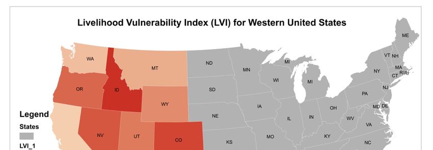
Fire 2021, 4, x FOR PEER REVIEW                                                                                                              4 of 32

                                    are further divided into sub-components (second level of divisions within each major
Fire 2021, 4, 54                                                                                                    4 of 29
                                    component) and subsequent indicator variables (measurable units of data for each sub-
                                    component) (Figure 1).

                 Description of
      Figure 1. Description     of the
                                   the framework
                                        framework developed
                                                    developed forfor the
                                                                      the LVI
                                                                          LVI (box 1 and the central gray circle). LVILVI is represented by
      contributing factor
                    factor(box
                             (box2).
                                  2).The
                                      Thecontributing
                                           contributingfactors
                                                         factorsare sensitivity
                                                                  are           (blue),
                                                                       sensitivity      exposure
                                                                                   (blue),        (red),
                                                                                           exposure      andand
                                                                                                     (red),  adaptive   capacity
                                                                                                                 adaptive        (green).
                                                                                                                            capacity      The
                                                                                                                                     (green).
      The  contributing   factors are  further divided  into major   components     (box 3). The major   components   are  color-coordinated
      contributing factors are further divided into major components (box 3). The major components are color-coordinated with
      with  the contributing
      the contributing         factors.
                         factors.        The major
                                  The major         components
                                              components          for sensitivity
                                                            for sensitivity  (blue)(blue)  are demographic,
                                                                                    are demographic,          ignition
                                                                                                       ignition        causes,
                                                                                                                 causes,        and environ-
                                                                                                                          and environmental
      mental   index (light  blue); for  exposure (red) are  wildfire  occurrence,   topography,   weather,  weather   extreme
      index (light blue); for exposure (red) are wildfire occurrence, topography, weather, weather extreme events (light        events (light
                                                                                                                                     red); for
      red); for adaptive capacity (green) are social network, natural, physical, human, and financial capital (light green). Major
      adaptive capacity (green) are social network, natural, physical, human, and financial capital (light green). Major components
      components are divided into sub-components (box 4) and represented by the sub-components in the outermost part of the
      are divided into sub-components (box 4) and represented by the sub-components in the outermost part of the circle. The
      circle. The sub-components are further divided into indicators (box 5) and not shown in this figure. Refer to Table A2 for
      sub-components
      each                 are further divided into indicators (box 5) and not shown in this figure. Refer to Table A2 for each
            indicator variable.
      indicator variable.
                                         In our study, the exposure factor pertains to wildfire danger and the physical pro-
                                         In our study, the exposure factor pertains to wildfire danger and the physical pro-
                                    cesses that influence the intensity and severity of fire behavior. Major components within
                                    cesses that influence the intensity and severity of fire behavior. Major components within
                                    exposure are wildfire occurrence, topography, weather, and extreme weather events. In
                                    exposure are wildfire occurrence, topography, weather, and extreme weather events. In
                                    our framework, an indicator variable under exposure is interpreted as variables that can
                                    our framework, an indicator variable under exposure is interpreted as variables that can
                                    adversely affect the exposure of wildfire risk to people within a state. For example, “total
                                    adversely affect the exposure of wildfire risk to people within a state. For example, “total
                                    acres burnt due to wildfires” is an indicator variable that represents how burnt soil dis-
                                    acres burnt due to wildfires” is an indicator variable that represents how burnt soil disturbs
                                    turbs hydrologic
                                    hydrologic         andconditions
                                                 and soil    soil conditions  leading
                                                                        leading         to increased
                                                                                  to increased        likelihood
                                                                                                likelihood         of flooding,
                                                                                                             of flooding,       runoff,
                                                                                                                           runoff,  and
                                    and  debris flow  [33]. This  variable can  be  interpreted  as, the greater  the  number  of
                                    debris flow [33]. This variable can be interpreted as, the greater the number of acres burnt, acres
                                    burnt, the greater
                                    the greater         the exposure
                                                the exposure   humanshumans
                                                                        have to have   to “knock-on”
                                                                                 “knock-on”            natural hazards,
                                                                                              natural hazards,            suchflooding
                                                                                                                 such as flash  as flash
                                    flooding  and landslides
                                    and landslides             within
                                                     within a state    a state
                                                                     (Table    (Table A2).
                                                                            A2).
                                          Sensitivity describes the degree to which each state is affected by wildfires. Its major
                                     components are demographic, ignition causes, and selected environmental indices. The
                                     indicator variables under sensitivity are interpreted as variables that contribute to a state’s
                                     sensitivity to wildfires. For example, the “number of houses within a wildland urban inter-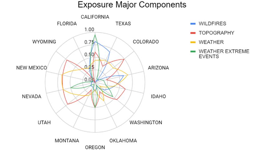
Fire 2021, 4, 54                                                                                          5 of 29

                   face zone” is an indicator variable under sensitivity because WUI are high-risk wildfire
                   regions due to their accumulation of wildland vegetation, concentration of flammable hu-
                   man structures, and potential ignition sources from sparks left by human activities [34,35].
                   Therefore, this indicator is interpreted as follows: States with larger WUI area and greater
                   number of homes within the WUI will be at increased risk and sensitivity to wildfires
                   (Table A2).
                         Adaptive capacity describes the ability of each state to withstand or recover from
                   wildfires. The major components of adaptive capacity include natural capital, physical
                   capital, human capital, social network, and financial capital. The indicator variables under
                   adaptive capacity are interpreted as variables that can positively contribute to the state’s
                   mitigation and adaptive strategies for wildfires. For example, “median household income”
                   is an indicator variable under adaptive capacity that can be interpreted as: States with
                   higher income may have more financial resources and financial capital to invest in home
                   and community hardening, thereby having higher mitigation and adaptation capacities
                   (Table A2).
                         When interpreting the indicator variables under each contributing factor (exposure,
                   sensitivity, and adaptive capacity), usually states with higher values would represent
                   greater exposure, sensitivity, or adaptive capacity to wildfires. For example, states with
                   higher temperatures would have a “greater exposure to wildfires”. However, for certain
                   indicator variables, the opposite is true, such as precipitation. States with higher amounts
                   of precipitation will have a “lower” exposure to wildfires. Indicator variables that are
                   interpreted as such require the inverse of their value to be integrated into the LVI equation
                   (e.g., instead of 12 mm of rain, it would be ( 121+1 ). These inverse indicators are denoted
                   with an asterisk (*) in Table A2. Please refer to Table A2 for a comprehensive overview of
                   our LVI framework that outlines all the major components, sub-components, and indicator
                   variables used in each contributing factor, along with detailed rationales and interpretation
                   on how we apply each indicator variable to assess the livelihood vulnerability of each state.

                   2.2. Input Variables
                         The LVI analysis is conducted solely for 14 fire prone American states that are most
                   at risk to wildfires. The states selected are Arizona, California, Florida, Idaho, Montana,
                   Nevada, New Mexico, Oklahoma, Oregon, Utah, Washington, and Wyoming because they
                   experienced the highest risk of wildfires in 2018, as determined from by the maximum
                   acres burnt in 2018 and 2019 and as documented in the NIFC 2019 Wildfire Risk Report
                   (Table A3 in the Appendix A). The 14 states analyzed in this study had the largest acreage
                   burnt in 2018 across the US (Figure 2). For these reasons, we limit our analysis to comparing
                   the LVI for only the top states most exposed to wildfires. The remainder of the states are
                   not as exposed and will inevitably provide irrelevant comparisons. Though Alaska was
                   included as a top state listed in the 2019 Wildfire Risk Report, it was excluded from our
                   study due to the lack of spatial and temporal comprehensive data, such as those required
                   under sensitivity (e.g., number of houses within the WUI zone), and if included, would
                   have impeded our comparison analysis among the other states.
                         Our analysis is conducted to determine the current LVI and not future LVI projections.
                   Therefore, most of the data gathered for our assessment were acquired within the past
                   decade (2010–2019). The exception is given to certain indicator variables that represent a
                   long-term climatological average (1950 to 2019). In addition, the elevation data for each
                   state was acquired from 1980, with the understanding that the elevation of each state
                   is not time sensitive and would not have changed drastically if the measurements were
                   acquired in 2019. The year in which the data was acquired for each indicator variable in
                   our framework is indicated in Table A2.
                         Furthermore, most of the data acquired are entered directly into the framework
                   as raw values, meaning that they did not require additional computations before the
                   LVI was calculated. However, some indicator variables under exposure, sensitivity, and
                   adaptive capacity required further processing to be amenable and included in the analysis.
Fire 2021, 4, 54 6 of 29
Indicator variables under the exposure that required initial computations included annual
average wind speed, humidity, annual precipitation, number of days with higher than
0.1 inches or more of precipitation, and annual temperature. The National Center for
Environmental Information (NCEI) provides annual averages of each indicator for various
weather observation stations located in each state. The values for every available weather
Fire 2021, 4, x FOR PEER REVIEW 6 of 32
observation station within each state were spatially averaged over the state and temporally
averaged over the 1950 to 2018 period before being used in our LVI calculations.
Figure 2.
Figure Map of
2. Map of the
theUnited
United States
States with
with the
thestates
states that
that are
are analyzed
analyzed shaded
shaded in in orange
orange and
and states
states not
not considered
considered shaded
shaded in
in
gray. The
gray. The acreage
acreage size
size burnt
burntinin2018
2018andand2019
2019isisindicated
indicated byby
thethe
redred
circles, ranging
circles, from
ranging thethe
from smallest circle
smallest (burn
circle areaarea
(burn less
thanthan
less 90,000 acres)
90,000 to the
acres) to largest circle
the largest (burn
circle areaarea
(burn exceeding 1 million
exceeding acres).
1 million acres).
The analysis
Our indicatorisvariables
conducted requiring initial computation
to determine the current LVIunder
andsensitivity
not futureincluded
LVI projec-the
Palmer Drought Index (PDI) and the number of smokers. The National
tions. Therefore, most of the data gathered for our assessment were acquired within the Oceanic and Atmo-
spheric
past Administration
decade (2010–2019).(NOAA) collects
The exception is monthly
given to PDI values
certain from weather
indicator variablesobservation
that repre-
sent a long-term climatological average (1950 to 2019). In addition, thecalculated
stations throughout the US every year. The 2019 annual average was for each
elevation data for
station and then averaged amongst all the stations within a state. We also
each state was acquired from 1980, with the understanding that the elevation of each state calculated the
isnumber
not timeof smokers using data from the United Health Foundation, which provided the
sensitive and would not have changed drastically if the measurements were
percentages of smokers for every state. To accurately convey the proportions between the
acquired in 2019. The year in which the data was acquired for each indicator variable in
states, the state’s population for that year was multiplied by its respective percentage of
our framework is indicated in Table A2.
smokers. Finally, for adaptive capacity, only the indicator variable pertaining to the total
Furthermore, most of the data acquired are entered directly into the framework as
area of lakes had to be computed. The original data provided the area for each individual
raw values, meaning that they did not require additional computations before the LVI
lake. Thus, we had to aggregate the area for all lakes to produce the cumulative lake area
was calculated. However, some indicator variables under exposure, sensitivity, and adap-
in each state.
tive capacity required further processing to be amenable and included in the analysis.
The motivation for including the selected indicator variables in our framework was
Indicator variables under the exposure that required initial computations included annual
based on current risk assessment information suggested by the open literature, such as
average wind speed, humidity, annual precipitation, number of days with higher than 0.1
potential health risks due to wildfires [36]. Other examples include indicator variables
inches or more of precipitation, and annual temperature. The National Center for Envi-
pertaining to fuel, weather, and topography that are important drivers of wildfire danger
ronmental
and behavior,Information
as referenced(NCEI) provides
heavily annual averages
in the literature of each indicator
[37,38]. Environmental for various
indices such as
weather observation
the PDI and stations
air quality located
were also in eachWhile
included. state.weThe values for every
acknowledge available
that there weather
are many fire
observation
indices that station
could be within each state
integrated were
[14], we spatially
selected PDIaveraged
because over
of its the state and
available tempo-
spatial and
rally averaged
temporal over
data for thestudy
our 1950and
to 2018 period
because PDIbefore beingindicator
is a useful used in our LVI calculations.
in describing an essential
The indicator variables requiring initial computation under
environmental factor (drought) required for the potential onset, ignition, and sensitivity included the
behavior
Palmer Drought Index (PDI) and the number of smokers. The National
of a wildfire [39]. Adding more fire indices and sub-indices would add redundancy to Oceanic and At-
mospheric Administration (NOAA) collects monthly PDI values from weather observa-
our framework.
tion stations throughout the US every year. The 2019 annual average was calculated for
each station and then averaged amongst all the stations within a state. We also calculated
the number of smokers using data from the United Health Foundation, which provided
the percentages of smokers for every state. To accurately convey the proportions between
the states, the state’s population for that year was multiplied by its respective percentage
of smokers. Finally, for adaptive capacity, only the indicator variable pertaining to the
total area of lakes had to be computed. The original data provided the area for each indi-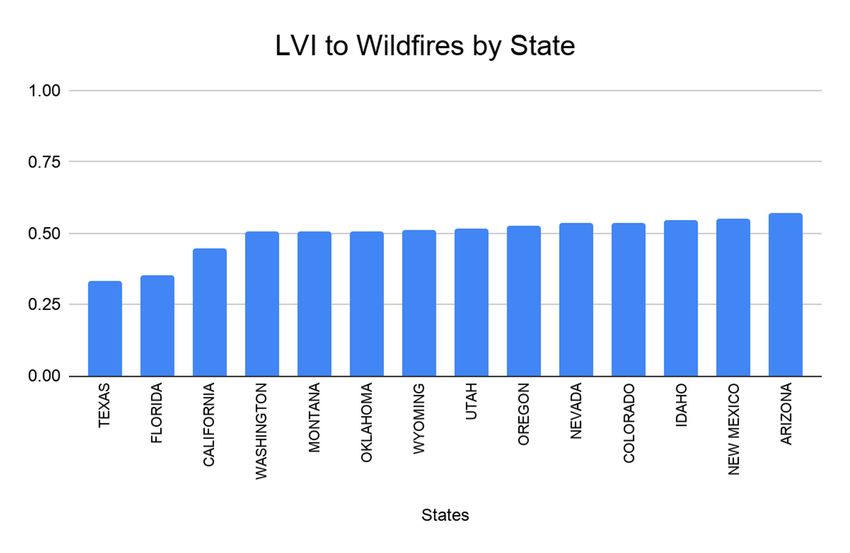
Fire 2021, 4, 54                                                                                            7 of 29

                   2.3. LVI Calculation
                         Subsequently, we calculate the LVI and the corresponding contributing factors for each
                   of the analyzed states based on our developed framework (Table A2). Our methods for
                   computing the LVI follows a similar approach to [18,27]. Before the computation, we need
                   to interpret whether the magnitude of each indicator value, under each contributing factor,
                   is influencing the contributing factor positively or negatively. If the indicator variable is
                   affecting the contributing factor negatively, then the inverse value is taken.
                         To compute LVI, we first compute the standardized index (SI) for each indicator
                   variable, where I, is the original indicator variable for each individual state, Imax and Imin
                   represent the state with the maximum and minimum value, respectively, corresponding to
                   that particular indicator, we use Equation (1).

                                                                 I − Imax
                                                        SI =                                                   (1)
                                                               Imax − Imin
                        Second, the major component (MC) value for each state is computed by averaging the
                   standard indices, over the number (n) of all indicators used in each major component, as in
                   Equation (2).
                                                                  ∑n SI
                                                        MC = i=1                                           (2)
                                                                    n
                        Third, each contributing factor (CF ) is computed by taking a weighted average of
                   each computed major component. This is done by multiplying each major component by
                   its number of indicators (Wi), as in Equation (3).

                                                                ∑[ MC ·Wi ]
                                                         CF =                                                  (3)
                                                                   ∑ Wi
                       Finally, the LVI for each state is computed by combining the contributing factors of
                   exposure ( E), adaptive capacity ( AC ), and sensitivity (S), as in Equation (4).

                                                        LV I = ( E − AC ) · S                                  (4)

                        The weighted balance function is applied to this method, as followed by [18]. The
                   weighted function gives equal weighting to each indicator variable, despite how many
                   indicators are present within the framework. This weighted approach is often used when
                   determining vulnerability in data-scare regions. Once the LVI is computed for each state, a
                   constant value of 0.5 is added to each LVI to simply aid in visualizing and interpreting the
                   rank of LVI [26].

                   2.4. Validation Framework Approach
                         We subsequently applied a PCA to our indicator variables in order to gain confidence
                   in the structure of our framework. PCA is a variable-reduction technique that takes a large
                   set of variables and organizes them into a smaller set of principal components. For the
                   purposes of this study, PCA was used to verify our framework by ensuring the indicator
                   variables were loading into the “proper” major components that they were assigned. When
                   conducting a PCA, four assumptions are made about the dataset, namely (1) the variables
                   are measured at the continuous level, (2) there is a linear relationship between the variables,
                   (3) there is adequate sample size, and (4) the dataset contains no outliers [40]. In addition,
                   two tests are conducted to determine whether PCA is a suitable method for validating our
                   framework: the Kaiser–Meyer–Olkin (KMO) sampling adequacy test [41] and Bartlett’s
                   Test of sphericity [42]. The KMO test measures the proportion of variance among the
                   indicator variables that may be caused by underlying factors. KMO is an average of the
                   measure of sample adequacy (MSA) for each indicator variable within their respective
                   major component. MSA values range from 0 to 1 and represent the extent of a given
                   indicator belonging to a group [43]. Smaller KMO values indicate fewer correlations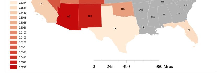
Fire 2021, 4, 54                                                                                             8 of 29

                   between a given variable and the other indicators. Therefore, if the KMO value is less than
                   0.5, the results from a PCA will not be useful because the indicators do not share high
                   correlations with each other. From Table A4 in the Appendix A, KMO values range mostly
                   between 0.5 and 0.8, suggesting a strong sampling adequacy. Bartlett’s test of sphericity
                   is conducted to determine whether the correlation matrix of the indicators is an identity
                   matrix. The null hypothesis is that the indicators are orthogonal (uncorrelated). For this
                   study, if the indicator variables are uncorrelated, then they are unsuitable for this factor
                   analysis. The values for this test range from 0 to 1, with 0 representing a rejection of the null
                   hypothesis (meaning that the indicator variables are correlated). In addition, a significance
                   value that is less than 0.05 indicates that PCA will provide helpful information. The values
                   for the Bartlett’s test of sphericity in our results mostly range from 0 to 0.3, suggesting that
                   the variables chosen are correlated. Table A4 in the Appendix A provides the KMO and
                   Bartlett test scores for each major component by using the indicator data gathered from the
                   14 states.
                         Once the indicator variables we selected had passed these tests, a PCA was conducted.
                   The normalized data input for PCA were the standardized values for each indicator. The
                   PCA gives insightful data such as a correlation matrix, communalities, and total variance
                   explained. However, the output that helped reorganize and strengthen our framework was
                   the component matrix. The component matrix displays the Pearson correlations between
                   the indicator variables and principal components. The component matrix was used to
                   verify whether the indicator variables loaded into their respective major components.
                   This indicates that they are measuring the same underlying construct and are, therefore,
                   correctly grouped accordingly in our framework.
                         Apart from the added confidence we gain from applying the PCA, we also conduct a
                   sensitivity analysis to test whether our framework provides robust livelihood vulnerability
                   results for each state. This is conducted by slightly perturbing our framework (through
                   randomly selecting to omit one indicator variable at a time from a major component)
                   and then re-running the LVI calculations. This will, thereby, provide twelve different
                   framework scenarios with LVI results generated for each state. The original LVI results
                   (current framework) is compared to the LVI output from each scenario to establish whether
                   the top three LVI states and the lowest three LVI states remain consistent throughout 90%
                   of the runs. If the LVI ranks remain the same (or are similar within reason) for more than
                   90% of the runs, these results provide additional validation to the framework. Refer to
                   Table A8 for a synthesis of the scenarios. We acknowledge that other scenarios may be
                   possible (by interchanging some indicator variables amongst the contributing factors) but
                   this would lead to many other possible scenarios and has already been tested by the PCA.

                   3. Results
                   3.1. LVI
                        We compute the LVI for each of the 14 American states analyzed (Figure 3). Most of
                   the states we analyzed exhibit similar LVI values. However, Arizona and New Mexico
                   experience the greatest livelihood vulnerability, with an LVI of 0.57 and 0.55, respectively.
                   In contrast, California, Florida, and Texas experience the least livelihood vulnerability to
                   wildfires (0.44, 0.35, 0.33, respectively) (Figure 4). To understand these LVI results, we
                   delve into analyzing each contributing factor.

                   3.2. Exposure
                        First, we examine each state’s susceptibility to wildfire by examining the exposure
                   contributing factor. The exposure results indicate that California, Nevada, and Arizona
                   exhibit the highest exposure to wildfires (0.63, 0.52 and 0.49, respectively) while Oklahoma,
                   Florida, and Montana have the least exposure (0.25, 0.21 and 0.19, respectively) (Figure 5a).
                   To understand the exposure results, we assess the four major components of exposure
                   (wildfire, topography, weather, and weather extreme events) for each state Figure 5b).
                   Wildfires (blue) is predominant for California, Texas, and Arizona. This is because these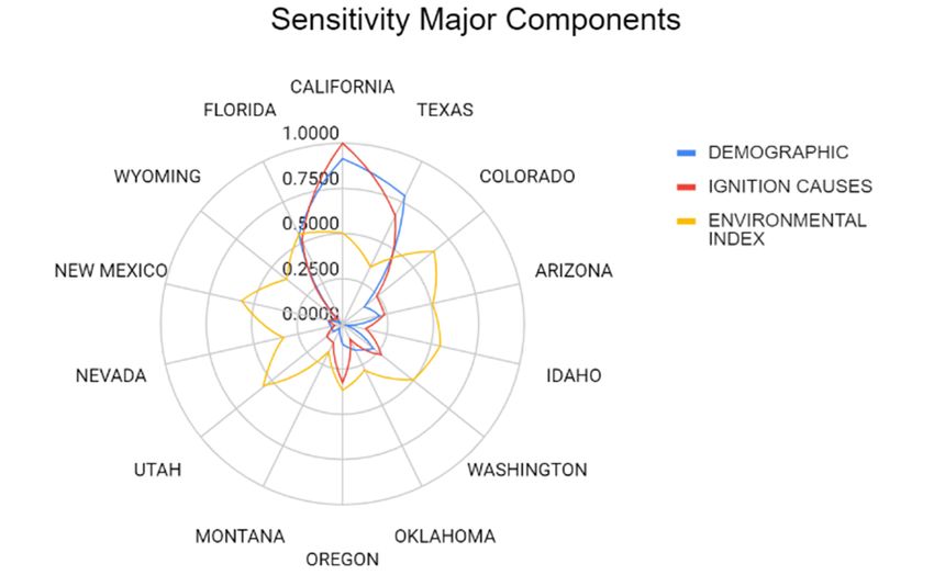
Fire 2021, 4, 54                                                                                                                   9 of 29

Fire 2021, 4, x FOR PEER REVIEW                                                                                                   9 of 32
  Fire 2021, 4, x FOR PEER REVIEW    states experience the highest number of wildfires and the largest acres burnt due to wildfires
                                                                                                                               9 of 32
                                     in 2019. Nevada and Arizona also experience relatively higher values of weather (yellow),
                                     which indicate favorable weather conditions for the development of wildfires, such as
                                    wildfires (0.44,
                                     relatively      0.35,
                                                higher     0.33,speeds
                                                         wind     respectively) (Figure
                                                                        and lower       4). ToInunderstand
                                                                                    humidity.               these LVI
                                                                                                 addition, weather    results,
                                                                                                                   extreme      we
                                                                                                                            events
                                     wildfires
                                    delve into  (0.44, 0.35,each
                                               analyzing      0.33, respectively)
                                                                 contributing     (Figure 4). To understand these LVI results, we
                                                                               factor.
                                     (green) represent extreme wildfire and extreme heat events and are most prevalent in
                                     delve into analyzing each contributing factor.
                                     California and Nevada.

     Figure 3. Map of each states’ LVI value, with its magnitude corresponding to the color bar where darker red indicates the
       Figure 3. Map of each states’ LVI value, with its magnitude corresponding to the color bar where darker red indicates the
     highest
       FigureLVI.  States
               3. Map     shaded
                       of each    grayLVI
                               states’ have not been
                                          value, with analyzed in thiscorresponding
                                                      its magnitude    study.       to the color bar where darker red indicates the
       highest
       highest LVI.
                LVI.States
                     Statesshaded
                            shadedgray
                                    grayhave
                                         havenot
                                              notbeen
                                                  beenanalyzed
                                                        analyzedin
                                                                 inthis
                                                                    thisstudy.
                                                                         study.

                                      Figure 4. Histogram showing the LVI of the 14 selected states in the US with Arizona having the
                                    Figure  4. LVI
                                      highest  Histogram  showing
                                                   and Texas havingthe
                                                                    theLVI   of the
                                                                          lowest    14 selected states in the US with Arizona having the
                                                                                 LVI.
                                    highest
                                      FigureLVI  and Texas having
                                              4. Histogram  showingthethe
                                                                        lowest LVI.
                                                                           LVI of the 14 selected states in the US with Arizona having the
                                      highest LVI and Texas having the lowest LVI.
                                    3.2. Exposure
                                      3.2.First,
                                           Exposure
                                                 we examine each state’s susceptibility to wildfire by examining the exposure
                                            First, we
                                    contributing      examine
                                                   factor.     each state’s
                                                           The exposure     susceptibility
                                                                         results           to wildfire
                                                                                 indicate that         by examining
                                                                                               California,          theArizona
                                                                                                           Nevada, and exposure
                                      contributing factor. The exposure results indicate that California, Nevada, and Arizona
these states experience the highest number of wildfires and the largest acres burnt due to
wildfires in 2019. Nevada and Arizona also experience relatively higher values of weather
(yellow), which indicate favorable weather conditions for the development of wildfires,
such as relatively higher wind speeds and lower humidity. In addition, weather extreme
Fire 2021, 4, 54 events (green) represent extreme wildfire and extreme heat events and are most prevalent
10 of 29
in California and Nevada.
(a) (b)
Figure5.5.Histogram
Figure Histogramshowing
showingthe theoverall
overallexposure
exposureofofthe
the1414selected
selectedstates
statesininthe
theUSUSwith
withCalifornia
Californiahaving
havingthe
thehighest
highest
exposure (with respect to wildland fire) and Texas having the lowest overall exposure (a). Radar plot showing the
exposure (with respect to wildland fire) and Texas having the lowest overall exposure (a). Radar plot showing the different different
majorcomponents
major componentsofofthetheexposure
exposurecontributing
contributingfactor,
factor,namely,
namely,wildfires
wildfires(blue),
(blue),topography
topography(red),
(red),weather
weather(yellow),
(yellow),and
and
weather extreme events (green) for the selected 14 states of the US (b).
weather extreme events (green) for the selected 14 states of the US (b).
Themajor
The majorcomponent,
component,topography,
topography,represents
representsmean
meanheight
heightand
andhighest
highestelevation
elevationfor
for
each state. Topography is important because higher elevations in complex
each state. Topography is important because higher elevations in complex terrain can be terrain can be
conducive to the propagation of wildfire behavior, add uncertainties to the prediction ofof
conducive to the propagation of wildfire behavior, add uncertainties to the prediction
thewildfire
the wildfirerate
rateofofspread
spread[44],
[44],and
andmake
makefirefiresuppression
suppressionefforts
effortsmore
morechallenging.
challenging.Thus,
Thus,
stateswith
states withhigher
highertopographic
topographicvalues
valuescould
couldpotentially
potentiallybebemore
moreatatrisk,
risk,orordangerously
dangerously
affectedby
affected bywildfires.
wildfires.Nevada
Nevadaalso alsoranks
rankshighhighinintopography.
topography.While
Whiletopography
topographyisisalso
also
relatively high for other states, such as Wyoming and Utah, other major
relatively high for other states, such as Wyoming and Utah, other major components, suchcomponents, such
aswildfires,
as wildfires,weather,
weather,andandweather
weatherextremes,
extremes,are arenegligible,
negligible,thereby
therebyreducing
reducingthetheoverall
overall
exposureofofwildfires
exposure wildfiresininthese
thesestates.
states.Furthermore,
Furthermore,Florida,
Florida,Oklahoma,
Oklahoma,and andMontana
Montanahavehave
thelowest
the lowestexposures
exposuresbecause
becauseallallofoftheir
theirmajor
majorcomponents
componentsunderunderexposure
exposureare areranked
ranked
verylow
very lowinincomparison
comparisontotothe theother
otherstates.
states.
3.3.
3.3.Sensitivity
Sensitivity
Second,
Second,weweassess
assessthe
thedegree
degreetotowhich
whicheach state
each is affected
state by wildfires
is affected by investigat-
by wildfires by investi-
ing the sensitivity
gating contributing
the sensitivity factor.factor.
contributing The results for sensitivity
The results (Figure(Figure
for sensitivity 6a) show
6a)California
show Cal-
as the most
ifornia sensitive
as the most state to wildfires
sensitive state to(0.84). This (0.84).
wildfires is followed
This by
is Texas, with
followed bya sensitivity
Texas, with ofa
0.66. Montana and Wyoming are the least sensitive. California, Texas, and
sensitivity of 0.66. Montana and Wyoming are the least sensitive. California, Texas, and Florida are the
most sensitive
Florida are thetomost
wildfires because
sensitive they yieldbecause
to wildfires the highest
theyvalues of each
yield the major
highest component
values of each
under sensitivity (demographic, ignition causes, and environmental
major component under sensitivity (demographic, ignition causes, and environmental index) (Figure 6b).
in-
Demographic comprises sub-components, such as the wildland-urban
dex) (Figure 6b). Demographic comprises sub-components, such as the wildland-urban interface (WUI) and
population.
interface (WUI)Statesand
with larger WUIStates
population. areaswith
or higher
largerpopulations
WUI areas within a WUI,
or higher would
populations
be more sensitive to wildfires because they are within a region more exposed
within a WUI, would be more sensitive to wildfires because they are within a region more to wildfire
events. Ignition causes attributed to outdoor activities, such as campfires and smoking,
would also increase the potential inception of human-caused fires. In addition, states that
experience poorer air quality and more drought will be more sensitive during and after
wildfire events and seasons. The environmental index remains relatively constant among
all states (yellow). However, California and Texas are the most sensitive states because they
are driven primarily by the major components of ignition causes (red) and demographic
(blue). The least sensitive state is Montana (0.08) because, in comparison to the other states,
all its major components are ranked relatively low.addition,
during states
and afterthat experience
wildfire eventspoorer air quality
and seasons. The and more drought
environmental willremains
index be morerelatively
sensitive
during and after wildfire events and seasons. The environmental index remains
constant among all states (yellow). However, California and Texas are the most sensitive relatively
constant
states among
because allare
they states (yellow).
driven However,
primarily by theCalifornia and Texasofare
major components the most
ignition sensitive
causes (red)
states because they are driven primarily by the major components of ignition causes
and demographic (blue). The least sensitive state is Montana (0.08) because, in comparison (red)
and demographic (blue). The least sensitive state is Montana (0.08)
to the other states, all its major components are ranked relatively low. because, in comparison
Fire 2021, 4, 54 11 of 29
to the other states, all its major components are ranked relatively low.
(a) (b)
(a) (b)
Figure 6. Histogram showing the overall sensitivity of the 14 selected states in the US with California having the highest
Figure6.6.Histogram
Figure
sensitivity Histogram showing
showing
(with respect theoverall
the
to wildland overall sensitivity
fire) sensitivity
and Texas ofofthe
the14
having 14 selected
selected
the statesininsensitivity
loweststates
overall theUS
the USwith
with California
California
(a). having
having
Radar plot thehighest
the
showing highest
the dif-
sensitivity
ferent major
sensitivity (with respect
components
(with respect toto wildland
of wildland fire)
the sensitivity and Texas
contributing
fire) and having the
factor,the
Texas having lowest
namely, overall
lowestdemographicsensitivity (a). Radar
(blue), (a).
overall sensitivity ignition
Radarplot
causesshowing
plot (red),
showing thethe
and dif-
the
ferent major
environmental components
index of
(yellow) the
forsensitivity
the selectedcontributing
14 states factor,
of the USnamely,
used indemographic
this study (blue),
(b). ignition causes
different major components of the sensitivity contributing factor, namely, demographic (blue), ignition causes (red), and the (red), and the
environmental index (yellow) for the selected 14 states of the US used in this study (b).
environmental index (yellow) for the selected 14 states of the US used in this study (b).
3.4. Adaptive Capacity
3.4. Adaptive Capacity
3.4. Adaptive
Third, weCapacity
assess the ability of each state to withstand or recover from wildfires by
Third,
analyzing
Third,thewe assessthe
theability
wecontributing
assess ability
factor ofofadaptive
eachstate
each state towithstand
withstand
capacity.
to orrecover
Our results
or recover
indicatefrom
fromthatwildfires
California,
wildfires by
by
analyzing
Texas, andthe
analyzing the contributing
Florida factor
exhibit factor
contributing of
the greatest adaptive
adaptive
of adaptive capacity. Our
capacity
capacity. results
Ourtoresults indicate
wildfires that
(0.69,that
indicate California,
0.67California,
and 0.48,
Texas,and
Texas, andFlorida
respectively) Florida exhibit
whileexhibit
Oregon, the
the greatest
Idaho, and
greatest adaptive
Montana
adaptive capacity to
are theto
capacity wildfires
least adaptive
wildfires (0.69, 0.670.12,
(0.15,
(0.69, 0.67 and0.48,
and 0.48,
0.12,
respectively) while
respectively) while
(Figure Oregon,
7a). The
Oregon, Idaho,
reasons
Idaho, and
andfor Montana are
the adaptive
Montana the least
are thecapacity adaptive (0.15,
disparities
least adaptive 0.12,
(0.15,among 0.12,
the
0.12, 0.12,
respectively)
states have to
respectively) (Figure
do with
(Figure 7a).
7a).the The
Themajor reasons
reasons for
components the adaptive capacity
(or capitals)
for the adaptive capacitythat disparities
each state
disparities among among
hasthe the
(natural,
states
states have
physical,
have to
to dohuman, do
with the with
social the major
network,
major components components
and financial) (or
Table
(or capitals) capitals) that each state has (natural,
A2.each state has (natural, physical,
that
physical,
human, human,
social socialand
network, network, and Table
financial) financial)
A2. Table A2.
(a) (b)
(a) (b)
Figure 7. Histogram showing the overall adaptive capacity of the 14 selected states in the US with California having the
highest adaptive capacity (with respect to wildland fire) and Texas having the lowest overall adaptive capacity (a). Radar
plot showing the different major components of the adaptive capacity contributing factor, namely, natural capital (blue),
physical capital (red), human capital (yellow), social network (green), and the financial capital (orange) for the selected
14 states of the US (b).
What drives the adaptive capacity to be relatively high for California and, to a slightly
lesser extent, Texas, are their social network (green) physical capital (red) and financial
capital (orange) (Figure 7b). These two states have social structures in place to facilitate
safety measures in times of wildfires such as allocating firefighters and first responders
to wildland fire emergencies. These states are also more equipped with transportationFire 2021, 4, 54 12 of 29
accessibilities, such as closer airports and access to public roads, in case of major wildfires.
California and Texas also have greater access to communication within their households,
including internet signals for receiving warning alerts, both of which can be beneficial
to one’s livelihood during the state of an emergency wildfire evacuation. These states
also rank highly in financial capital, such as having relatively higher household incomes
and fire management assisted grants, which can lend financial support during wildland
fire emergency hazards. Additionally, Florida also has a high adaptive capacity that is
primarily driven by its natural capital. It has the largest water area of all the states analyzed,
thereby providing the state with water resources for fire suppression.
In contrast to the states with the highest adaptive capacity, Montana, Idaho, and
Oregon rank very low in all capitals. Moreover, while some states rank high in one major
component, it suffers in others, thereby driving down the rank of its overall adaptive ca-
pacity value. For example, New Mexico has a relatively high human capital in comparison
to other states, which corresponds to residential density and occupation; however, all its
other capitals are negligible, resulting in an overall low adaptive capacity to wildfires. This
emphasizes the need to evaluate all the contributing factors in adaptive capacity to obtain
a holistic view of the allotted resources available to aid in wildfire resiliency measures.
Adaptive capacity is one of the most important determining factors in risk assessment, as
highlighted by [45]. who showed that wildfire hazard potential can be reduced once the
adaptive capacity of the state is taken into consideration.
4. Discussion
4.1. Validation of Framework
4.1.1. Principal Component Analysis (PCA)
A PCA was conducted for each major component to test the indicators categorized
within them. Table A4 in the Appendix A shows the results after running the KMO and
Bartlett test. All of the values from the KMO test are at least 0.5, which is the minimum
required value to conduct a PCA as described in [41]. The only major component that
is not at least 0.5 is that of weather, which has a value of 0.488. Previous research such
as [46] suggests a KMO value of at least 0.6 in order to proceed with PCA. However, due
to the small sample size and indicators tested per PCA (adaptive capacity, 13; exposure,
11; sensitivity, 9) it is difficult to achieve a KMO value of at least 0.6. In addition, in
this study, PCA was not utilized for its typical purpose of reducing variables, but rather,
performed to verify whether the indicators within each major component loaded onto one
principal component.
Table A4 in the Appendix A also contains the results for the Bartlett test. Some of the
major components achieved a desirable value of less than 0.05. However, some had values
higher than 0.05. This is not an issue for two reasons. First, the major components that
had a value greater than 0.05 had only two indicators to test. Only having two variables
to create a correlation matrix would make it very difficult to achieve a value below 0.05.
Second, the purpose of conducting a Bartlett test is to assess whether the correlation matrix
diverges significantly from an identity matrix for data reduction [47]. Since the goal of the
PCA is not variable reduction, the correlation matrix only needed to be proven as not being
an identity matrix, that is, a value closer to 0 than 1.
After computing the PCA, we analyzed the generated component matrices. To val-
idate the framework, the indicators had to have a strong loading into their respective
major components. A strong loading is considered to be any value above 0.5 and sug-
gests that the indicators are measuring the same underlying construct. Despite the fact
that a PCA was conducted for each major component, the results are compiled into three
tables (Tables A5–A7 in the Appendix A), one for each contributing factor. Overall, most
of the indicators demonstrated a strong loading into their respective major components.
However, there were some indicators that had weak loadings, under a value of 0.5, for
example, annual average wind speed and annual average temperature in exposure. These
indicators had a factor loading of 0.17 and 0.39, respectively, for the major component ofFire 2021, 4, 54 13 of 29
weather. These low values indicate an inverse relationship between the other indicators
under weather [48]. When a state is characterized by higher wind speed and temperature,
they are more likely to be exposed to wildfires. The other indicators under weather involve
humidity and precipitation. If a state is characterized by higher humidity and precipitation,
then they are less likely to be exposed to wildfires in that same year. The same logic can be
applied to the following indicators: acres of forests, number of timber/woodworkers, and
annual PDI. These indicators all have negative loadings for their respective major compo-
nents. These inverse relationships were reflected in the calculation of the LVI. With PCA
verifying the structure of our framework, the validity of the LVI results is strengthened.
4.1.2. Sensitivity Analysis
Another test to validate our framework, included a sensitivity analysis. We perturbed
the framework by removing one indicator variable at time and testing the rank of the new
LVI results. A total of twelve scenarios were conducted (Table A8). Under exposures, the
indicators removed were wildfire occurrence, mean height above sea level, wind speed, and
extreme heat. Despite these exposure perturbations, the LVI rank for the top three (Arizona,
New Mexico, Idaho) and lower three LVI states (Texas, Florida, California) remained the
same as the original LVI outputs.
Similarly, the same analysis was carried out for sensitivity for which indicators: WUI
area, number of campsites, and the air quality index were removed. The LVI results did
not vary for these scenarios. Applying this approach to adaptive capacity, one indicator
variable was removed at a time under each major component (area of lakes, miles of public
roads, persons per household, number of firefighters, median household income). While
the results remained the same for most perturbed scenarios of adaptive capacity, omission
of the median household income changed the top LVI rank to include Colorado and not
Idaho. The top LVI states were, Arizona, Colorado, followed by New Mexico. However,
the lower three LVI states remained the same.
Overall, only one of the 12 scenarios showed a slight shift in the LVI rank for one of
the states, but the top two (Arizona, and New Mexico) were still ranked accordingly. The
results remained consistent for 92% of the runs. The results from this sensitivity analysis
provides validation on applying our framework to quantify livelihood vulnerability.
4.2. Contribution of LVI
The main findings indicate that Texas, Florida, and California exhibit the lowest
livelihood vulnerability to wildfires, while Idaho, New Mexico, and Arizona experience
the greatest. Assessing each contributing factor and its respective major components and
subcomponents have provided an in-depth analysis of why the livelihood vulnerability
of some states to wildfires are higher than others. Many media and scientific reports
constantly show California as the state with the most dangerous and destructive wildfires,
especially in recent years. The NIFC report showed that California had the highest acres
burned and maximum damages in 2018 among all the states. According to the 2019–2020
California Budget Summary [49], approximately ten of the most destructive wildfires
in California have occurred since the year 2015. Thus, one might think that California,
with the highest exposure, would have the highest LVI. Our study indicates that, while
California is the most exposed, and sensitive to wildfires (Figure 8), it has a very high
adaptive capacity to help offset its livelihood vulnerability. The California Administration
has implemented solutions and recommendations to reduce wildfire risk to improve the
state’s emergency preparedness, response, and recovery capacity, and to further protect
vulnerable communities. The 2019–2020 state budget includes 918 million dollars in
additional funding to comply with these efforts [49]. For these reasons, it is evident why
California exhibits a lower livelihood vulnerability to wildfires, relative to other states.You can also read