Interactions between deforestation, landscape rejuvenation, and shallow landslides in the North Tanganyika-Kivu rift region, Africa - Earth ...
←
→
Page content transcription
If your browser does not render page correctly, please read the page content below
Earth Surf. Dynam., 9, 445–462, 2021
https://doi.org/10.5194/esurf-9-445-2021
© Author(s) 2021. This work is distributed under
the Creative Commons Attribution 4.0 License.

               Interactions between deforestation, landscape
              rejuvenation, and shallow landslides in the North
                     Tanganyika–Kivu rift region, Africa
        Arthur Depicker1 , Gerard Govers1 , Liesbet Jacobs1 , Benjamin Campforts2 , Judith Uwihirwe3,4 , and
                                                 Olivier Dewitte5
                              1 KU Leuven, Department of Earth and Environmental Sciences,

                  Division of Geography and Tourism, Celestijnenlaan 200E, 3001 Heverlee, Belgium
         2 CSDMS, Institute for Arctic and Alpine Research, University of Colorado at Boulder, Boulder, CO, USA
                           3 University of Rwanda, Department of Soil and Water Management,

                           Faculty of Agricultural Engineering, Street KK 737, Kigali, Rwanda
                    4 Delft University of Technology, Faculty of Civil Engineering and Geosciences,

                      Department of Water Management, Stevinweg 1, 2628 Delft, The Netherlands
                            5 Royal Museum for Central Africa, Department of Earth Sciences,

                                      Leuvensesteenweg 13, 3080 Tervuren, Belgium
                            Correspondence: Arthur Depicker (arthur.depicker@kuleuven.be)

                                Received: 20 October 2020 – Discussion started: 26 October 2020
                           Revised: 21 April 2021 – Accepted: 27 April 2021 – Published: 31 May 2021

      Abstract. Deforestation is associated with a decrease in slope stability through the alteration of hydrological
      and geotechnical conditions. As such, deforestation increases landslide activity over short, decadal timescales.
      However, over longer timescales (0.1–10 Myr) the location and timing of landsliding is controlled by the in-
      teraction between uplift and fluvial incision. Yet, the interaction between (human-induced) deforestation and
      landscape evolution has hitherto not been explicitly considered. We address this issue in the North Tanganyika–
      Kivu rift region (East African Rift). In recent decades, the regional population has grown exponentially, and the
      associated expansion of cultivated and urban land has resulted in widespread deforestation. In the past 11 Myr,
      active continental rifting and tectonic processes have forged two parallel mountainous rift shoulders that are
      continuously rejuvenated (i.e., actively incised) through knickpoint retreat, enforcing topographic steepening.
      In order to link deforestation and rejuvenation to landslide erosion, we compiled an inventory of nearly 8000
      recent shallow landslides in © Google Earth imagery from 2000–2019. To accurately calculate landslide ero-
      sion rates, we developed a new methodology to remediate inventory biases linked to the spatial and temporal
      inconsistency of this satellite imagery. Moreover, to account for the impact of rock strength on both landslide
      occurrence and knickpoint retreat, we limit our analysis to rock types with threshold angles of 24–28◦ . Rejuve-
      nated landscapes were defined as the areas draining towards Lake Kivu or Lake Tanganyika and downstream of
      retreating knickpoints. We find that shallow landslide erosion rates in these rejuvenated landscapes are roughly
      40 % higher than in the surrounding relict landscapes. In contrast, we find that slope exerts a stronger control on
      landslide erosion in relict landscapes. These two results are reconciled by the observation that landslide erosion
      generally increases with slope gradient and that the relief is on average steeper in rejuvenated landscapes. The
      weaker effect of slope steepness on landslide erosion rates in the rejuvenated landscapes could be the result of
      three factors: the absence of earthquake-induced landslide events in our landslide inventory, a thinner regolith
      mantle, and a drier climate. More frequent extreme rainfall events in the relict landscapes, and the presence of a
      thicker regolith, may explain a stronger landslide response to deforestation compared to rejuvenated landscapes.
      Overall, deforestation initiates a landslide peak that lasts approximately 15 years and increases landslide erosion
      by a factor 2 to 8. Eventually, landslide erosion in deforested land falls back to a level similar to that observed

Published by Copernicus Publications on behalf of the European Geosciences Union.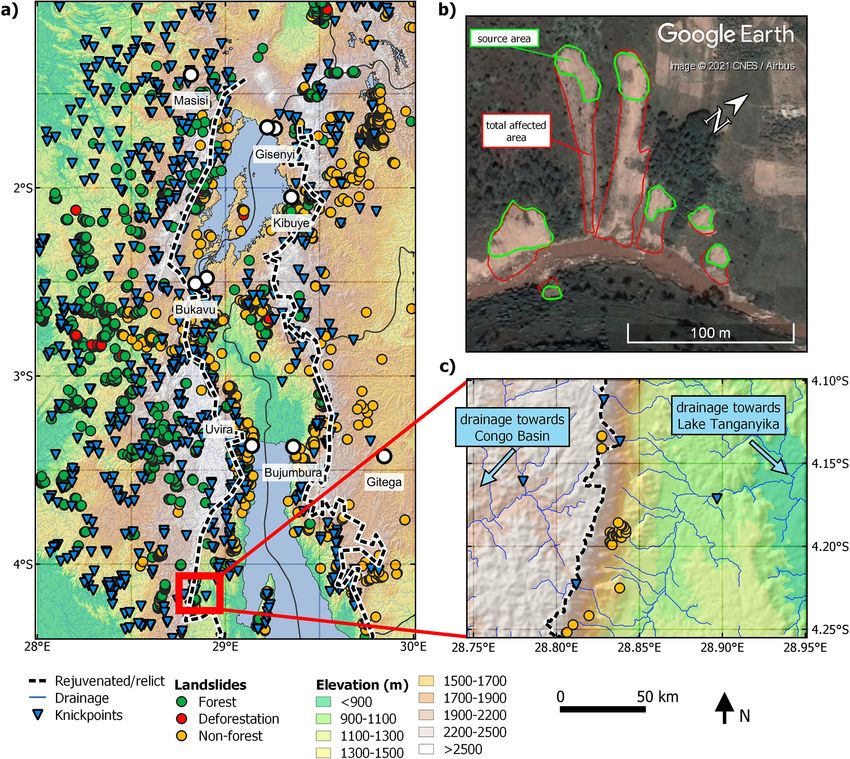
446                                              A. Depicker et al.: Deforestation, rejuvenation, and landslides in the Kivu rift

       under forest conditions, most likely due to the depletion of the most unstable regolith. Landslides are not only
       more abundant in rejuvenated landscapes but are also smaller in size, which may again be a consequence of a
       thinner regolith mantle and/or seismic activity that fractures the bedrock and reduces the minimal critical area for
       slope failure. With this paper, we highlight the importance of considering the geomorphological context when
       studying the impact of recent land use changes on landslide activity.

1   Introduction                                                   continental rifting (Hansen et al., 2013; Saria et al., 2014;
                                                                   Monsieurs et al., 2018a; Depicker et al., 2020; Dewitte et al.,
On steep terrain, the erosion caused by shallow landslides         2021). The study area is therefore an ideal setting to eval-
(with a maximal depth of a couple of meters) increases sig-        uate how deforestation affects landslide erosion in different
nificantly as a result of deforestation (e.g. Montgomery et al.,   landscape settings.
2000; Mugagga et al., 2012). The removal of trees, due to
either human or natural causes, decreases the slope stabil-        2   The North Tanganyika–Kivu rift region
ity through the alteration of hydrological and geotechnical
conditions, such as the loss in soil cohesion due to tree root     Active continental rifting in our study area is driven by the
decay (Sidle et al., 2006; Sidle and Bogaard, 2016). After         divergence of the Victoria and Nubia plates that started at ca.
10–20 years, depending on the climate and vegetation regen-        11 Ma and currently continues at a rate of ca. 2 mm/yr (Saria
eration rate, this effect starts wearing off (Sidle and Bogaard,   et al., 2014; Pouclet et al., 2016). Due to this setting, there
2016). However, when forests are permanently converted to          is widespread seismic activity, active volcanism, and uplift,
grassland or cropland, the consequences of deforestation for       initiating landscape rejuvenation through knickpoint retreat
landsliding can last much longer or even be permanent (Sidle       (Smets et al., 2015; Delvaux et al., 2017; Dewitte et al.,
et al., 2006).                                                     2021). Adding to the geological complexity of the NTK rift
   While these general principles are well described, we do        is the wide variability in age and strength of rock formations.
not yet fully understand the extent to which the response to       The majority of rocks in the northern and eastern parts of
deforestation is modulated by tectonic forcing, which typ-         the study area are of Mesoproterozoic age (1600–720 Ma),
ically occurs over timescales of 0.1–10 Myr (e.g. Whipple          being mostly quartzites, granites, or pelites. The southwest
and Meade, 2006). A key distinction can be made here be-           is largely covered by either weathering-resistant quartzites
tween actively incising, rejuvenating landscapes, in which         or weathering-prone gneiss and micaschists of Paleoprotero-
landslides are a prime slope-limiting mechanism and “old”,         zoic age (2500–1600 Ma). Within the rift shoulders, the same
so-called relict landscapes, where hillslopes have had a long      pattern of Meso- and Paleoproterozoic rocks is observed,
time to adapt to river incision (Burbank et al., 1996; Larsen      save for the occurrence of much younger lithologies such
and Montgomery, 2012). These two landscape types can be            as the river and lake sediments in the Ruzizi floodplain and
expected to respond differently to deforestation: in rejuvenat-    the volcanic deposits (12 Ma–present) found around Bukavu
ing landscapes, hillslopes are already continuously adapting       and north of Goma (Delvaux et al., 2017; Laghmouch et al.,
to river incision through landsliding (Egholm et al., 2013).       2018).
In relict landscapes, on the other hand, hillslopes will slowly       In the natural context, prior to widespread human activity,
become less steep and landslides will occur more sporadi-          forests covered most of the DRC and the mountainous rift
cally, potentially allowing for a thick regolith mantle to de-     shoulders in Rwanda and Burundi, while the vegetation tran-
velop (Schoenbohm et al., 2004; Bennett et al., 2016). Cli-        sitioned to woodland savanna towards the east of our study
matic variations can also drive differences in landscape re-       area (Ellis et al., 2010; Aleman et al., 2018; Roche and Nza-
sponse to deforestation (Crozier, 2010), and in the context of     bandora, 2020). Only since the beginning of the 20th century
lithologically diverse landscapes, the effect of rock strength     has large-scale deforestation taken place, especially along the
on both knickpoint retreat and landsliding must also be ac-        rift shoulders and in Rwanda and Burundi (Ellis et al., 2010;
knowledged (Parker et al., 2016; Baynes et al., 2018; Camp-        Aleman et al., 2018). In 2000, the study area (ca. 88 500 km2 )
forts et al., 2020).                                               had an estimated forest coverage of 73.1 %. Between 2001
   Here, we aim to explore the interplay of deforestation and      and 2018, 4.5 % of this forest was cleared, mainly for the
uplift-driven landscape rejuvenation on shallow landslide          purpose of agriculture (Hansen et al., 2013; Tyukavina et al.,
erosion. We focus our research on the North Tanganyika–            2018; Musumba Teso et al., 2019). Deforestation is there-
Kivu rift region (hereafter referred to as “the NTK rift”,         fore an indirect result of the fast-growing population, which
Fig. 1), part of the western branch of the East African Rift.      increased from 89 inhabitants per km2 in 1975 to 241 inhabi-
The area is characterized by frequent landsliding, mostly          tants per km2 in 2015 (Hansen et al., 2013; JRC and CIESIN,
triggered by rainfall, widespread deforestation and active         2015).

Earth Surf. Dynam., 9, 445–462, 2021                                                  https://doi.org/10.5194/esurf-9-445-2021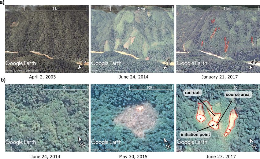
A. Depicker et al.: Deforestation, rejuvenation, and landslides in the Kivu rift                                                       447

Figure 1. Overview of the North Tanganyika–Kivu (NTK) rift. (a) Extent of the studied area and active faults (Delvaux and Barth, 2010).
LANDSAT-8 imagery is used as background (USGS, 2018). (b) The transects of the elevation at different latitudes illustrate the elevated rift
shoulders, being the result of tectonic uplift. The four most populous cities in the area of the NTK rift (Goma, Bukavu, Uvira, Bujumbura)
are located in between the rift shoulders. The transect was derived from the 30 m resolution digital elevation model (DEM) provided by the
Shuttle Radar Topography Mission (SRTM) (USGS, 2006).

3     Methods                                                           data, we distinguish three land cover classes: (i) forest, hav-
                                                                        ing > 25 % tree cover (as suggested by Hansen et al., 2013);
In the sections below, we first focus on the landscape charac-          (ii) deforested land; and (iii) non-forest land, with ≤ 25 %
teristics of the NTK rift that can exert a control on landslide         tree cover. Both deforested and non-forest land encompass
erosion: forests, rejuvenation, rainfall, and rock strength.            land use classes such as bare land, cropland, grassland, and
Next, we elaborate on the different aspects of the landslide            urban land. Historically, current non-forest land used to be
erosion assessment: the compilation of an inventory and the             either savanna grassland or forest (Roche and Nzabandora,
calculation of shallow landslide erosion rates (in the context          2020). The difference between non-forest land that used to
of the previously determined landscape characteristics).                be forested in the past and deforested land is the elapsed time
                                                                        since deforestation. Thus, the non-forest land either under-
3.1     Regional controls on landslide erosion                          went deforestation before the year 2000 or was never forest
                                                                        in the first place. Deforested land experienced deforestation
3.1.1    Forest cover and deforestation                                 over the last 2 decades.
We characterize the NTK rift in terms of forest dynamics by
means of the global forest data presented by Hansen et al.              3.1.2    Landscape rejuvenation
(2013) (Fig. 2a; the data were updated in 2018). This dataset
contains a tree cover map for the year 2000 and forest loss             To distinguish the rejuvenated landscapes within the rift
data for the period 2001–2017, both provided at a resolution            shoulders from the surrounding landscapes (hereafter re-
of 1 arcsec (ca. 30 m). The tree cover data show the percent-           ferred to as the relict landscapes), we use the spatial pattern
age of tree coverage per pixel in 2000, and the forest loss             of knickpoints retreating upstream towards the rift shoulders,
data display discrete values between 1 and 17, indicating               away from the active faults. Stationary knickpoints, here de-
the year in which deforestation took place. Based on these              fined as knickpoints at a distance shorter than 1 km from a ge-

https://doi.org/10.5194/esurf-9-445-2021                                                       Earth Surf. Dynam., 9, 445–462, 2021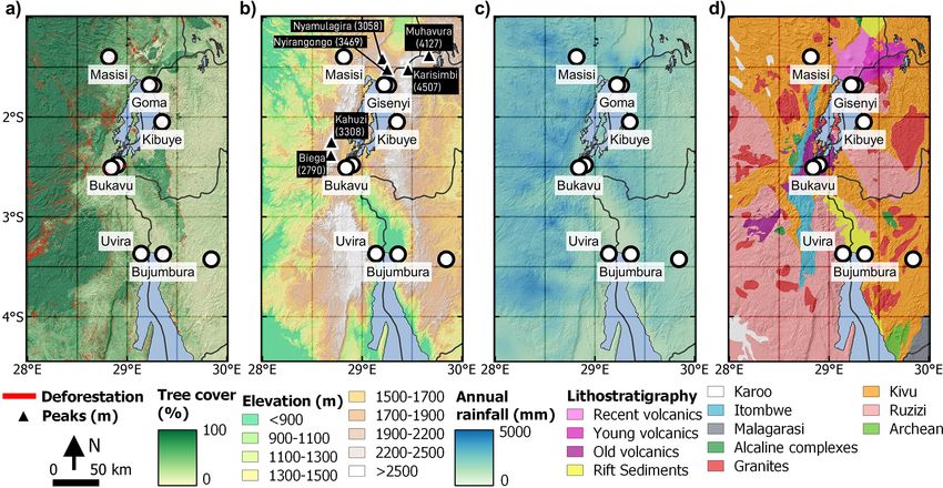
448 A. Depicker et al.: Deforestation, rejuvenation, and landslides in the Kivu rift
Figure 2. Environmental characterization of the NTK rift: (a) tree cover for the year 2000 and deforestation from 2001–2017 (Hansen et al.,
2013), (b) elevation and some renowned mountain peaks (height expressed in meters) (USGS, 2006), (c) average annual rainfall between
2005–2015 (Van de Walle et al., 2020); (d) lithostratigraphy (Table 1) (Laghmouch et al., 2018).
ological contact, are considered unrelated to the rejuvenation rainfall events in the NTK rift. Moreover, field observations
process and removed from the analysis (Kirby and Whipple, and local reports confirm that the majority of recent shallow
2012; Bennett et al., 2016). Two criteria are applied to iden- landslides are rainfall-triggered (Monsieurs et al., 2018a; De-
tify the rejuvenated rift: (i) the area must drain towards Lake picker et al., 2020; Dewitte et al., 2021). To explore any re-
Kivu or Lake Tanganyika, and (ii) the area must be located lationship between rejuvenation and rainfall, we analyze two
downstream of any non-stationary knickpoint unless there is metrics: the average annual rainfall and the number of times
no knickpoint observed in the area. In the latter case, we as- when accumulated rainfall was sufficiently large to trigger
sume the knickpoint reached the rift shoulder and the land- landsliding. As a proxy of the latter criterion, we use a 2 d,
scape is completely rejuvenated. 15 mm threshold as it is a conservative estimation for global
We use the KNICKPOINTFINDER function in TopoToolbox thresholds set by Guzzetti et al. (2008). Our intent is not
to identify knickpoints. This function requires a drainage net- to approximate an actual in situ threshold but rather to re-
work and tolerance value, reflecting the maximum expected flect spatial patterns in intense rainfall capable of triggering
error in the true river profiles (Schwanghart and Scherler, landslide events. For the comparison of rainfall patterns be-
2017). The drainage network for this purpose is modeled tween rejuvenated and relict landscapes, we apply the non-
with the 1 arcsec SRTM DEM data (USGS, 2006) and a parametric Mann–Whitney U test, whereby each observation
threshold catchment area of 2 × 10⁶ m2 . The tolerance value is the average metric (rainfall or threshold exceedance) in
is used to distinguish knickpoints from discrepancies in the fifth-order catchments. These units are derived from the 30 m
longitudinal river profile that are caused by errors in the DEM using a river catchment threshold of 105 m2 .
DEM data. The tolerance value is calculated as the maxi- The rainfall pattern is derived from a regional climate sim-
mal difference between the 90th and 10th quantile of the ulation with COSMO-CLM, a physical model, for the period
smoothed river profiles (Schwanghart and Scherler, 2017) 2005–2015 and using the ERA5 reanalysis product for the
and subsequently lowered until the algorithm identifies the initial and boundary conditions of the atmosphere (Van de
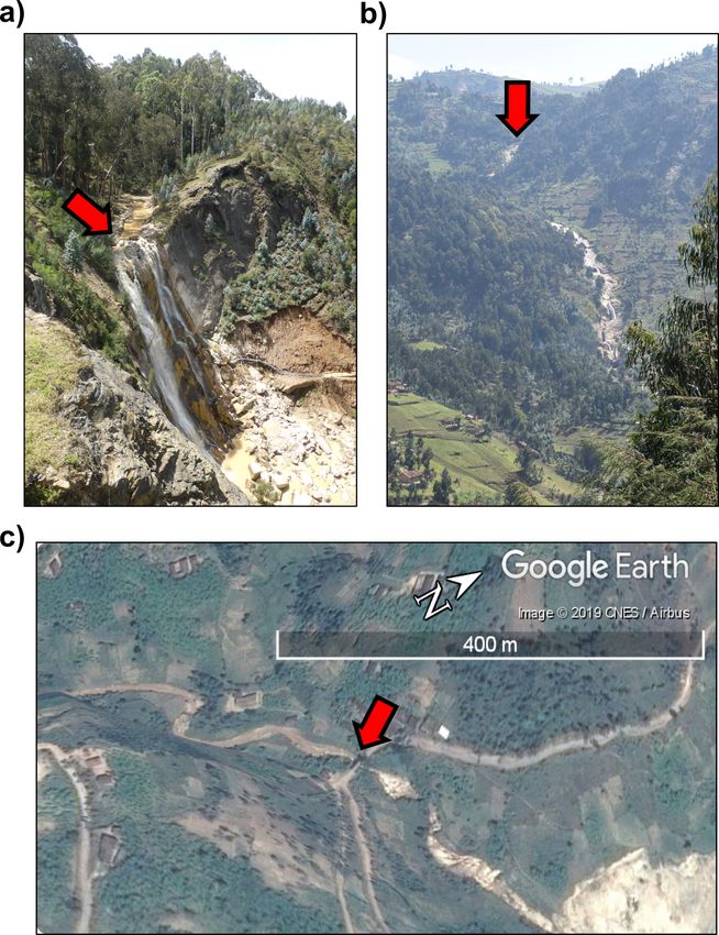
three knickpoints we validated in the field (Fig. 3). Walle et al., 2020; Hersbach et al., 2020). Due to in situ data
scarcity, evaluation of the simulated precipitation amounts
3.1.3 Rainfall is restricted to a comparison with a set of satellite products.
Generally, the satellite data suggest lower amounts of rainfall
Active rifting not only triggers landscape rejuvenation but compared to the simulated model output (Van de Walle et al.,
also impacts local rainfall patterns (Van de Walle et al., 2020), yet this was expected as satellite products tend to un-
2020). Depicker et al. (2020) showed a significant link be- derestimate actual precipitation (Dinku et al., 2011; Mon-
tween landslide occurrence and the frequency of extreme
Earth Surf. Dynam., 9, 445–462, 2021 https://doi.org/10.5194/esurf-9-445-2021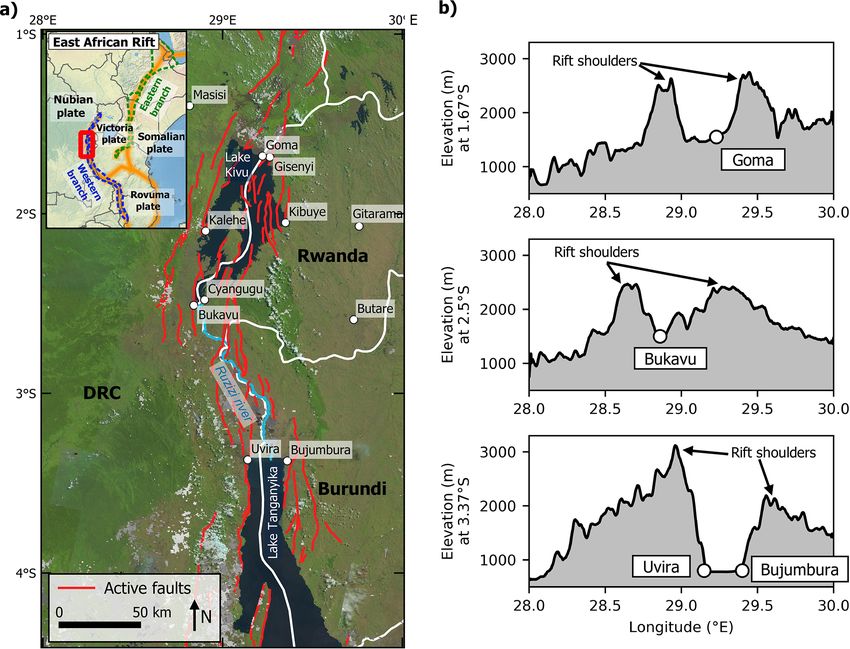
A. Depicker et al.: Deforestation, rejuvenation, and landslides in the Kivu rift                                                 449

                                                                     et al., 2020). We determine the rock strength by analyz-
                                                                     ing the dependency of the mean hillslope gradient, S, on
                                                                     the normalized steepness index, ksn , averaged on a catch-
                                                                     ment scale (Safran et al., 2005; DiBiase et al., 2010; Bennett
                                                                     et al., 2016). We analyze first-order catchments, whereby a
                                                                     drainage network was derived from the 1 arcsec SRTM DEM
                                                                     data and a threshold catchment area was set at 105 m2 , i.e.,
                                                                     large enough so that the smallest rivers visible in © Google
                                                                     Earth were detected. For each lithostratigraphical unit, we
                                                                     only consider watersheds where more than 50 % of the area
                                                                     is covered with the dedicated lithostratigraphy.
                                                                        The ksn values of a river segment is a proxy for the river
                                                                     incision rate and is calculated using the following equation
                                                                     (Wobus et al., 2006):

                                                                     ksn = Schan Aθref ,                                          (1)

                                                                     where Schan is the local channel slope, A is the upstream
                                                                     catchment area, and θref is the reference concavity index,
                                                                     for which we assume a value of 0.45 (see, e.g., DiBiase and
                                                                     Whipple, 2011).
                                                                        Theory suggests a positive linear relationship between S
                                                                     and ksn in catchments with relatively low river incision rates.
                                                                     For catchments with high river incision rates, an increase in
                                                                     ksn will not lead to further hillslope steepening but to slope
                                                                     failure (DiBiase et al., 2010; Korup and Weidinger, 2011;
                                                                     Larsen and Montgomery, 2012), and thus the S becomes in-
Figure 3. Field-validated knickpoints in Rwanda. The red ar-
                                                                     dependent of the ksn . To capture this nonlinear dependency
row indicates the location of the knickpoint: (a) east of Mabanze,   of average basin slope on channel steepness, we introduce a
Rwanda (2.047852◦ S, 29.469678◦ E); (b) east of Kanama, Rwanda       new empirical relationship to describe the response of S to
(1.705683◦ S, 29.391763◦ E); (c) southwest of Kibilira, Rwanda       ksn :
(1.980443◦ S, 29.61586◦ E). Image © 2019 Google Earth.
                                                                                            a
                                                                     S = TA 1 − exp −          ksn ,                             (2)
                                                                                           TA
sieurs et al., 2018b). The final model output has a spatial res-
olution of 2.8 km and a temporal resolution of 1 h (Fig. 2c).        where parameter a is the slope of the curve at ksn = 0. Thus,
Note that the spatial resolution of the rainfall products might      for low incision rates, a approximates the slope of the linear
be too low to fully capture the impact of orographic controls        relationship between S and ksn . Parameter TA is the slope an-
and the local convective storm patterns (Monsieurs et al.,           gle to which the terrain converges for high ksn values. Hence,
2018b).                                                              TA can be considered equivalent to the threshold slope. How-
                                                                     ever, when there is a linear relationship for S = f (ksn ) in the
                                                                     entire ksn range (when the R 2 > 0 for a linear fit), we do not
3.1.4   Rock strength and threshold slopes                           consider the threshold estimate reliable.
In order to account for the control of lithology on the hill-
slope response to uplift and incision (Schmidt and Mont-             3.2     Quantifying shallow landslide erosion
gomery, 1995; Korup, 2008; Korup and Weidinger, 2011;                3.2.1    Inventory
Bennett et al., 2016), we classify the 12 lithostratigraphical
units present in the NTK rift (Fig. 2d and Table 1) into major       The assessment of shallow landslide erosion is based on a
categories based upon the analysis of their threshold slope, a       © Google Earth landslide inventory, which is an update from
proxy for rock strength (Korup and Weidinger, 2011). Rock            the dataset presented by Depicker et al. (2020). Only recent
strength is a factor that must be taken into account when in-        landslides, for which we can estimate the time of occurrence,
vestigating landslide characteristics; equal slopes with dif-        are considered in our inventory. In other words, the moment
ferent rock strength properties are expected to display dif-         of failure must be situated between the timing of two images.
ferent behavior in terms of landsliding and knickpoint re-           Moreover, since deforestation mainly affects the stability of
treat (Parker et al., 2016; Baynes et al., 2018; Campforts           the first few meters of the regolith (Sidle and Bogaard, 2016),

https://doi.org/10.5194/esurf-9-445-2021                                                   Earth Surf. Dynam., 9, 445–462, 2021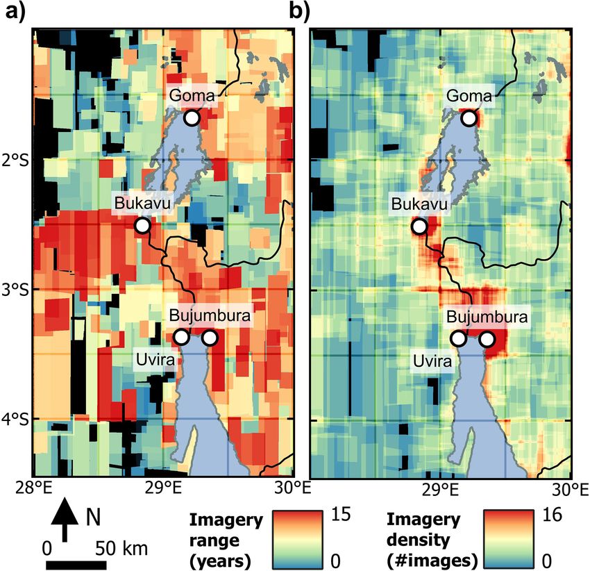
450                                                A. Depicker et al.: Deforestation, rejuvenation, and landslides in the Kivu rift

Table 1. Lithostratigraphical units in the NTK rift as presented by Depicker et al. (2020) and based on the work of Laghmouch et al. (2018).

  Age                Chronostratigraphy    Lithostratigraphy          Main lithological constitution
  10 Ka–present      Late Quaternary       Recent volcanics           Lava, tuff, and ash, deposited in the past decades and centuries, a
                                                                      result of eruptions of the Nyiragongo and Nyamulagira.
  2–1 Ma             Early Quaternary      Young volcanics            Relatively fresh basalts, deposited at ± 2 Ma.
  12–6 Ma            Neogene               Old volcanics              Highly weathered basalt, deposited at 11–4 Ma.
  23 Ma–present      Late Cenozoic         Rift sediments             Sand along the lake or swamps more inland.
  360–201 Ma         Karoo                                            Black shales, tillite, not metamorphosed.
  1000–540 Ma                              Itombwe                    Black shales, tillite, silicified tillite, weakly methamorphosed.
                     Neoproterozoic
                                           Malagarasi                 Black shales, tillite, silicified tillite, weakly methamorphosed. Pres-
                                                                      ence of dolomites and volcanic rocks (basalts).
  820–720 Ma                               Alcaline complexes         Granitic rocks, intrusive volcanic rocks (rhyolite).
                     Mesoproterozoic
  1375–980 Ma                              Granites                   Two-mica and leucogranites.
  1600–1000 Ma                             Kivu                       Pelites, quartzopelites, and quartzites at different degrees of weath-
                                                                      ering. Moderately metamorphosed.
  2500–1600 Ma       Paleoproterozoic      Ruzizi and ante-Ruzizi     Gneiss and micaschists, prone to chemical weathering, and
                                                                      quartzites, resistant to weathering. Strongly methamorphosed.
  4000–2500 Ma       Archaen                                          Gneiss and micaschists, prone to chemical weathering, and
                                                                      quartzites, resistant to weathering.

Figure 4. Examples of deforestation followed by landsliding. The left column shows the area prior to deforestation. The middle column
shows the area after deforestation but prior to landsliding. The right column shows the area after landsliding. (a) Landslide event north of
Butezi, DRC (2.843201◦ S, 28.296984◦ E; image © 2019 Google Earth). (b) Landslide event in Matale, DRC (2.645874◦ S, 28.360656◦ E;
image © 2019 Google Earth).

Earth Surf. Dynam., 9, 445–462, 2021                                                         https://doi.org/10.5194/esurf-9-445-2021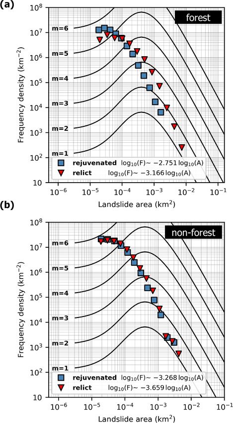
A. Depicker et al.: Deforestation, rejuvenation, and landslides in the Kivu rift                                              451

                                                                                                        j
we only consider shallow landsliding in this study. Deep-          r j . The LSF in each subarea LSF is then
seated and bedrock landslides are excluded from the inven-
tory. We apply a maximum depth of a couple of meters for              j      nj
                                                                   LSF =         ,                                             (4)
landslides to be inventoried. We estimate the relative depth of            rj Aj
the landslides (shallow or deep-seated) through in situ field
observations and/or by visually analyzing the shape and size       with nj the number of landslides in subarea j , Aj the sur-
of the landslide scarp and deposits in © Google Earth im-          face area of j , and r j the constant imagery range in j . To
agery (Depicker et al., 2020). All images used in the analysis     calculate the frequency for the entire study area, the frequen-
                                                                          j
are of very high spatial resolution, ranging from 30 to 60 cm.     cies LSF are averaged out using weights proportional to their
The images in © Google Earth are provided by either © Dig-         corresponding area Aj :
italGlobe or © CNES/© Airbus, and they were captured be-
                                                                           N
tween 2000 and 2019. Each landslide is manually assigned a                 X Aj           j
                                                                   LSF =              LSF ,                                    (5)
polygon delineating the source area so that the total source                      A
                                                                           j =1
area LSS can be calculated (m2 km−2 yr−1 ; Sect. 3.2.2). The
LSS is the area over which regolith material has been re-             with N the number of subareas j . Substituting Eqs. (4) and
moved by landsliding on an annual basis and serves as a            (5) becomes
proxy for shallow landslide erosion. We also manually assign
a point of initiation used to calculate the landslide frequency               N
                                                                           1X     nj
LSF (no. of LS km−2 yr−1 ; Sect. 3.2.2) to each landslide. In      LSF =              .                                        (6)
                                                                           A j =1 r j
order to calculate the LSF as accurately as possible and avoid
amalgamation, we differentiate between separate source ar-
eas (Li et al., 2014; Marc et al., 2015; Roback et al., 2018).     Hence, we do not require the size Aj of each subarea j for
We also pay attention to inventory landslides not linked to        the calculation of the total LSF . Instead of aggregating the
mining and quarrying. Such sites were identified either dur-       LSF over all subareas, we can aggregate the LSF over the
ing fieldwork or in © Google Earth imagery through charac-         individual landslides. Eq. (6) then becomes
teristics such as a gradual growth of the affected area over a                n
                                                                           1 X   1
time span of several years and the presence of mining infras-      LSF =             ,                                         (7)
tructure (road tracks, trucks, buildings, spoil tips) within the           A i=1 r i
affected area.
   The one-sided Mann–Whitney U test is applied to statis-         with r i the time range observed in landslide i. The landslide
tically quantify any differences between different landslide       inventory is expected to be biased due to spatial differences
populations (McDonald, 2014). Furthermore, we illustrate           in the imagery density d (Fig. 5b), defined as the total number
the potential differences between the landslide areas of re-       of available images at each location, as vegetation regrowth
juvenated and relict landscapes by comparing the frequency         might erase the spectral signature of landslides before they
density of the landslide areas. The frequency density curves       are captured in imagery. Hence, we expect to detect more
are fitted to the inverse 0 distribution (Malamud et al., 2004).   landslides in areas with higher imagery density. To compen-
                                                                   sate for this bias, we assume that the probability of identi-
                                                                   fying a landslide in a certain region increases linearly with
3.2.2   Calculating landslide erosion rates from a biased          imagery density in that specific region. Equation (7) then be-
        © Google Earth inventory                                   comes
                                                                              n
Generally, the LSF is calculated as follows:                               1 X     1
                                                                   LSF =               ,                                       (8)
                                                                           A i=1 r d i
                                                                                  i

         n
LSF =      ,                                                (3)
        rA                                                         with d i the imagery density observed at the location of land-
                                                                   slide i. Note that there can be a saturation of the information
with n the total number of shallow landslides, A the total area    provided by the imagery: when the imagery density is high,
(km2 ), and r the imagery range (years) in © Google Earth,         the availability of one extra image will have no to little ef-
i.e., the age difference between the oldest and youngest im-       fect on the observed number of landslides. We validate our
age. The imagery range is thus equal to the period of observa-     assumptions of linearity and saturation by visually assessing
tion. However, the imagery range is highly variable through-       the dependency of landslide density (number of landslides
out the study area due to differences in the availability of       per square kilometer) on imagery density. If the assumption
© Google Earth imagery (Fig. 5a). Since Eq. (3) is valid           of linearity does not hold, we have to apply a non-linear
when r is constant within our study area, we divide our study      transformation on the d i values. If saturation is problematic
area in subareas j that each have a constant imagery range         to our inventory, we have to set a maximum value for d i .

https://doi.org/10.5194/esurf-9-445-2021                                                      Earth Surf. Dynam., 9, 445–462, 2021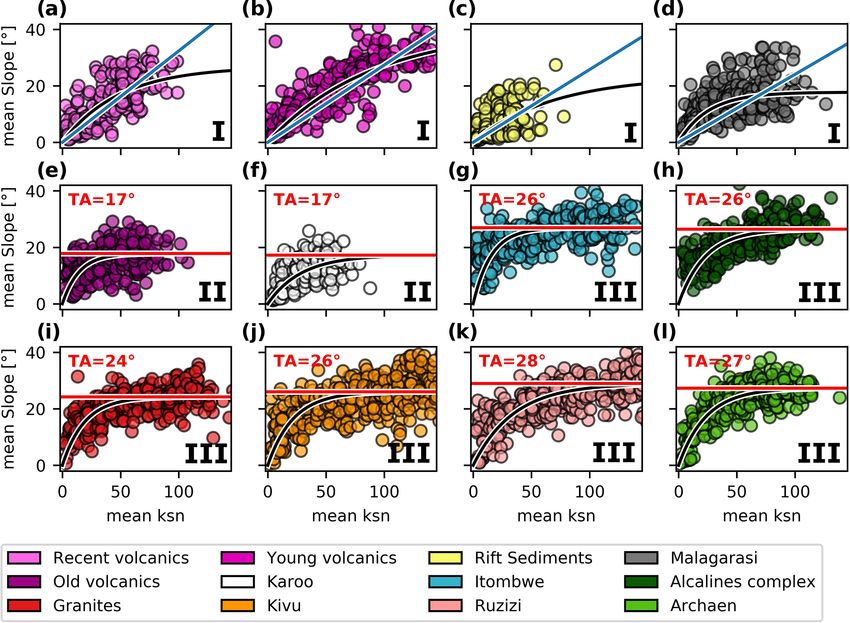
452                                                A. Depicker et al.: Deforestation, rejuvenation, and landslides in the Kivu rift

                                                                      3.2.3   Impact of slope on landslide erosion

                                                                      In order to assess the impact of slope steepness on the LSS
                                                                      (a proxy for landslide erosion), we first reclassify the slope
                                                                      values between 0–50◦ into 10 classes of equal width and sub-
                                                                      sequently apply Eq. (10) to each slope class and the land-
                                                                      slides therein. Similarly, to assess the impact of slope steep-
                                                                      ness on LSF , we apply Eq. (8) to each slope class and its land-
                                                                      slides. Furthermore, we estimate the degree to which our LSS
                                                                      and LSF calculations are affected by outliers and/or extreme
                                                                      landslide events. First, we divide the study area in 50 east–
                                                                      west bands of equal width. Second, we calculate the LSS and
                                                                      LSF for each slope class 50 times, each time leaving out the
                                                                      slope and landslide data for a single east–west band. In other
                                                                      words, for each run we slightly perturbate the landslide in-
                                                                      ventory.

                                                                      3.2.4   Linking forest cover and deforestation to landslide
                                                                              erosion
Figure 5. Visualization of the imagery bias in © Google Earth prior
to 4 May 2019: (a) imagery range and (b) imagery density. The         In order to link forest dynamics to landslide erosion, we must
range and density were calculated by manually identifying 932 im-     distinguish between landslides that followed deforestation
agery footprints. The highest imagery density is available for the    (Fig. 4) and landslides that caused deforestation. To iden-
major cities in the study area (Goma, Bukavu, and Bujumbura),         tify the correct causality, we reconstructed the timeline of
whereas the northwest and southwest regions have fewer observa-       every landslide that occurred on deforested land (Fig. 6b).
tions. For some areas (in black) there is no available image.         Landslides following deforestation are defined as those that
                                                                      happened within the post-deforestation time range, being the
                                                                      period between the first image after the year of deforestation
  Deriving the LSS equations is analogous to deriving the             and the most recent image.
ones for the LSF . We only have to slightly modify Eq. (7)               Determining the LSS as a function of the time elapsed
and Eq. (8):                                                          since deforestation (tdef ) is necessary to characterize the post-
                                                                      deforestation landslide wave. Because tdef is temporally dy-
           n   i
        1 X  asrc                                                     namic, this analysis requires two components: (i) the total
LSS =             ,                                            (9)
        A i=1 r i                                                     area Atdef in which we can observe land that was deforested
                                                                      tdef years ago and (ii) the total affected area of landslides that
                                                                      happened tdef years after deforestation. The first component,
           n     i                                                    Atdef , entails all areas where the sum of tdef and the year of de-
        1 X    asrc
LSS =                 ,                                       (10)    forestation lies in the time range between the age of the oldest
        A i=1 r i d i                                                 and newest post-deforestation image in © Google Earth. For
                                                                      the second component, we only include landslides for which
whereby asrci is the source area of landslide i. Note that the        the time between deforestation and landsliding (tdef→LS ) is
calculation of LSS will be less accurate than for the LSF             equal to tdef .
due to biases in the delineation of the landslide source area.           There is a considerable degree of uncertainty associated to
These biases are caused by the time lag between the land-             tdef→LS since we do not know the exact timing of the land-
slide occurrence and the landslide detection in © Google              slides (the occurrence is situated between the capture times
Earth, whereby part of the source area might already have             of the image where it was initially observed and the preced-
recovered. To avoid biases linked to the interpretation of            ing image). Similarly, we know the year of deforestation but
the source area, all landslides were delineated by the same           not the exact date. To assess the uncertainty on the timing
person. In order to statistically verify a difference in land-        of deforestation and landslide occurrence, we calculate the
slide activity between regions (for example rejuvenated ver-          LSS 100 times, each time sampling a new tdef→LS for each
sus relict landscapes), we use the one-sided non-parametric           landslide. For each sample of tdef→LS , we make two assump-
Mann–Whitney U test to compare the different landslide ac-            tions: (i) the exact moment of deforestation (the lower limit
tivity measures in fifth-order water catchments (calculated           of tdef→LS ) is assumed to be distributed uniformly in the re-
with Eqs. 8 and 10 to compensate for imagery density differ-          ported deforestation year. (ii) The timing of landslide occur-
ences).                                                               rence (the upper limit of tdef→LS ) is assumed to be distributed

Earth Surf. Dynam., 9, 445–462, 2021                                                     https://doi.org/10.5194/esurf-9-445-2021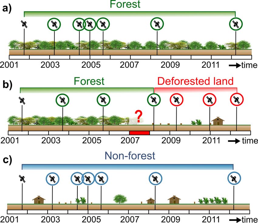
A. Depicker et al.: Deforestation, rejuvenation, and landslides in the Kivu rift                                                      453

                                                                            tense (potentially landslide-triggering) rainfall events occur
                                                                            less frequently.
                                                                               Based on the analysis of 234 840 first-order catchments,
                                                                            we identify three major lithological categories (Fig. 8). Cat-
                                                                            egory I comprises units that do not display clear threshold
                                                                            angles. These are lithostratigraphies of relatively young age
                                                                            such as recent and young volcanic basalts and lake and river
                                                                            sediments (all < 23 Myr), except for the Malagarasi rock for-
                                                                            mations. The latter formations are of old age (1000–540 Ma)
                                                                            and cover only a small area in the southeast of the study area.
                                                                            The lack of threshold landscapes in Category I could be re-
                                                                            lated to the relatively short duration of exposure to weath-
                                                                            ering for these rocks. Category II, consisting of old vol-
                                                                            canic basalts and Karoo lithostratigraphy (both younger than
                                                                            210 Myr), has threshold slopes of roughly 17◦ . Rocks of Cat-
                                                                            egory III, with observed threshold slopes ranging between
                                                                            24–28◦ , are generally of older age (> 540 Myr) and display a
Figure 6. Schematic overview of the three considered forest cover
                                                                            high resistance to slope failure. The lithostratigraphy of Cat-
scenarios in © Google Earth. The satellite icons signal the avail-          egory III includes the following formations: Itombwe, Alca-
ability of a © Google Earth image, and the colored circles indicate         line complexes, Granites, Kivu, Ruzizi, and Archaen.
whether we can potentially observe recent landslides in the con-
cerned image. Panel (a) shows the forest scenario, wherein each             4.2   Shallow landslide erosion in the NTK rift: impacts of
landslide observed in these areas is linked to forest cover. Panel (b)
                                                                                  deforestation and rejuvenation
shows the deforestation scenario, wherein only landslides observed
starting from the second © Google Earth image after the year of             We inventoried 7944 recent shallow landslides (Fig. 7a). Fol-
deforestation are considered to be linked to deforestation (in other        lowing the classification of Hungr et al. (2014), the observed
words, we can only observe deforestation-induced landslides in im-          landslides were mostly debris slides, caused by the sliding
agery that is encircled in red on the figure). Hence, in this illustrated
                                                                            of regolith on a planar surface parallel to the ground. These
example, we cannot attribute landslides from the 2008 imagery to
deforestation, as we cannot be sure that these landslides happened
                                                                            debris slides, once initiated, often transform into avalanches,
before or after the 2007 deforestation. Note that we do not know the        characterized by the flow of (at least partially) saturated de-
exact moment of deforestation, only the year (indicated with the red        bris on a steep slope. Another commonly observed landslide
bar) is reported. Panel (c) shows the non-forest scenario, wherein          type was the debris or mud flow, defined as the rapid flow
every landslide observed in these regions is linked to non-forest ar-       of saturated debris in a steep channel. In total, we found 873
eas.                                                                        landslides in deforested land, yet we could only be certain
                                                                            for 378 of those landslides that they were preceded by de-
                                                                            forestation (Sect. 3.2.4). Furthermore, 3155 landslides were
uniformly between the capture times of the image where it                   associated with forest, and 4411 landslides were associated
was initially observed and the preceding image.                             with non-forest. Rocks of Category I and II combined con-
                                                                            tained only 344 instances, hampering a robust analysis. We
                                                                            therefore focus our further analysis on the 7600 landslides in
4     Results                                                               areas with rocks of Category III.
                                                                               The number of observed landslides in © Google Earth
4.1    Regional controls on landslide erosion                               appears to increase linearly with the available imagery up
                                                                            to a density of 12 images (Fig. 9a). The proportion of the
We identified 673 non-stationary knickpoints using a toler-                 study area with a higher density than 12 images is negli-
ance value of 100 m. These knickpoints were used to demar-                  gible (1.5 %) and contains merely 1 % of all landslides in
cate the rejuvenated landscapes inside the rift (Fig. 7a). The              the inventory. Hence, the assumption that landslide density
rejuvenated landscapes encompass 15 526 km2 , i.e., 18 % of                 is linearly dependent on imagery density is valid within our
the entire study area.                                                      study area, and we take no measures to correct for saturation
   The average annual rainfall in the rejuvenated land-                     (Sect. 3.2.2). The annual extent of imagery made available
scapes is significantly lower than in the relict landscapes                 in © Google Earth increases with time, especially after 2010
(1905 mm/year versus 2297 mm/year, p < 0.01). Similarly,                    (Fig. 9b).
we find that within the rejuvenated landscapes, the 2 d,                       After accounting for differences in imagery density, the
15 mm threshold is exceeded less often compared to the relict               overall LSS in rejuvenated landscapes, which is a proxy for
landscapes (17 % difference, p < 0.01), indicating that in-                 shallow landslide erosion, is roughly 40 % higher than in

https://doi.org/10.5194/esurf-9-445-2021                                                         Earth Surf. Dynam., 9, 445–462, 2021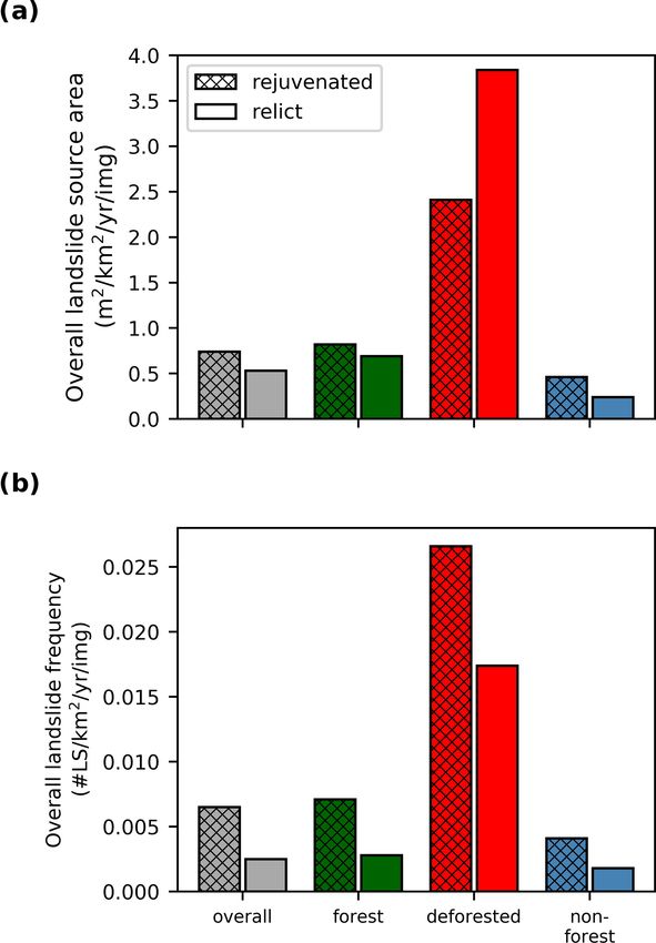
454                                                  A. Depicker et al.: Deforestation, rejuvenation, and landslides in the Kivu rift

Figure 7. Landslide and knickpoint inventory for the NTK rift. (a) We identified 7994 shallow recent landslides that occurred either in forest,
non-forest, or after deforestation and 673 non-stationary knickpoints. These knickpoints were used to separate the rejuvenated landscapes
between the rift shoulders from the surrounding relict landscapes (black and white line). (b) Example of shallow landslides in Rwanda
(−1.7151◦ S, 29.7909◦ E) and the delineation of their total area (red) and source area (green). (c) Example of the rift shoulder west of Lake
Tanganyika. The method for delineating the rejuvenated landscapes is specified in Sect. 3.1.2.

relict landscapes (p = 0.034, Fig. 10a). The difference be-               weathering and sediment deposition are outpaced by erosion
comes even larger when looking at the LSF (160 %, p =                     (Montgomery, 2001; Dykes, 2002; Prancevic et al., 2020).
0.014, Fig. 10b), which implies that landslides are on av-                When comparing slopes of equal steepness, we observe that
erage smaller in rejuvenated landscapes. This difference in               the LSS is generally higher in relict landscapes than in reju-
landslide size between rejuvenated and relict landscapes is               venated landscapes (Fig. 12c). Nevertheless, the overall LSS
confirmed in all three land cover types: forests (114 versus              is higher in rejuvenated landscapes because the overall pre-
308 m2 , p < 0.01, Fig. 11a), non-forests (111 versus 138 m2 ,            dominance of steeper relief (Fig. 12g, h) compensates for
p < 0.01, Fig. 11b), and deforested land (94 versus 239 m2 ,              the fact that comparing similarly angled individual slopes in
p < 0.01). Similar to the rejuvenation status, forest cover               rejuvenated and relict zones, rejuvenated slopes are shown
also influences the landslide size. The average source area               to have a lower or equal rate of shallow landslide erosion
for forests (223 m2 ) decreases non-significantly after defor-            (Fig. 12c).
estation (165 m2 , p = 0.06). In non-forest lands, the land-                 Recently deforested slopes are up to 8 times more sensitive
slide size (126 m2 ) is significantly smaller than in recently            to shallow landsliding compared to forested slopes (Fig. 12a,
deforested lands (p < 0.01).                                              b). The deforestation effect lasts approximately 15 years
   The LSS and LSF increase with slope gradient (Fig. 12a, b,             (Fig. 13). However, deforestation increases LSS much more
d, e). A decrease is observed for forested slopes > 45◦ , which           in relict landscapes compared to rejuvenated areas (Fig. 12c).
could be linked to limitations on regolith formation, whereby             The LSS in the non-forested areas (blue lines in Fig. 12) cor-

Earth Surf. Dynam., 9, 445–462, 2021                                                          https://doi.org/10.5194/esurf-9-445-2021
A. Depicker et al.: Deforestation, rejuvenation, and landslides in the Kivu rift                                                            455

Figure 8. Threshold slope analysis for the different lithostratigraphical units in the NTK rift. Each point represents a first-order river catch-
ment over which we averaged the slope gradient S and normalized river steepness index ksn . The black curves represent the S = f (ksn )
relationship fitted to Eq. 2. (a)–(d) Category I: young lithostratigraphy for which no clear threshold angle is observed. (e)–(f) Category II:
young lithostratigraphy with a low threshold angle of ca. 17◦ . (g)–(l) Category III: older rocks with higher observed threshold slopes of
24–28◦ .

responds to the situation that prevails once the deforestation-            on longer timescales due to the occurrence of major landslide
induced landslide wave has passed. In this situation, the LSS              events triggered by large earthquakes (Delvaux and Barth,
drops back to a level similar to that observed under forest                2010; Marc et al., 2015). However, in our observed period,
(green line) (Fig. 12a, b).                                                chances of earthquake-triggered landsliding were very lim-
                                                                           ited (Dewitte et al., 2021). The lack of such observations sug-
                                                                           gests that our window of observation was too short to capture
5     Discussion
                                                                           earthquakes that were large enough to trigger landsliding.
                                                                           Over the long term, the contribution of earthquake-induced
5.1    Interactions between deforestation, rejuvenation,
                                                                           landsliding to regolith mobilization in the rejuvenated land-
       and landslide erosion
                                                                           scapes may nevertheless be important. Earthquakes fracture
While the landslide erosion rate (approximated by the LSS )                and weaken the hillslope material and hence reduce the min-
is higher in rejuvenated landscapes due to a steeper relief, the           imum critical area for landslide initiation (Delvaux et al.,
relative effect of slope steepness on landslide erosion appears            2017; Milledge et al., 2014; Vanmaercke et al., 2017). As
to be weaker in rejuvenated landscapes: we found that steep                such, seismic activity may also contribute to a smaller av-
(> 35◦ ) forested slopes display higher shallow landslide ero-             erage landslide size in rejuvenated landscapes. Moreover, a
sion rates in relict landscapes than in rejuvenated landscapes             previous study in the NTK rift established an indirect link
(Fig. 12c). We evaluate three mechanisms that could explain                between spatial patterns of seismic activity (approximated
this difference: seismic activity, regolith availability, and cli-         by a modeled peak ground accelaration (PGA) product by
mate.                                                                      Delvaux et al., 2017) and the spatial pattern of the landslide
   Seismic activity is a first factor that could explain why               occurrence, though this study did not differentiate between
slope has a different impact on landslide erosion in reju-                 deep-seated and shallow landsliding (Depicker et al., 2020).
venated and relict landscapes. Generally, there is more and                   A second factor potentially contributing to the differ-
stronger seismic activity within the rejuvenated landscapes                ence in slope impact on erosion rates in rejuvenated and
(Delvaux et al., 2017). We hypothesize that the higher seis-               relict landscapes (Fig. 12c) is that the regolith mantle on
mic activity would result in elevated landslide erosion rates              rejuvenated slopes is expected to be thinner and less con-

https://doi.org/10.5194/esurf-9-445-2021                                                          Earth Surf. Dynam., 9, 445–462, 2021
456 A. Depicker et al.: Deforestation, rejuvenation, and landslides in the Kivu rift
Figure 9. The impact of imagery density (the number of available
images in © Google Earth) on the number of observed landslides.
We only show the results for the rocks of Category III (Sect. 4.1).
Therefore, major cities that are characterized by a high imagery den-
sity like Bukavu, Bujumbura, and Goma are excluded from this fig-
ure. (a) Impact of the imagery density on the number of observed
landslides. The number of landslides seems to increase linearly with
imagery density up to 12 images. The cumulative landslide propor- Figure 10. Total landslide activity in the NTK rift adjusted for im-
tion for a certain value shows the percentage of the landslide inven- agery density: (a) total landslide source area (LSS ), a proxy for
tory contained in areas with an imagery density equal or lower than landslide erosion, and (b) landslide frequency (LSF ).
that value. (b) The evolution of imagery availability between 2000
and 2018.
steepness in relict landscapes (Fig. 12c) but also a higher
LSF . The latter is not the case: slope steepness appears to
tinuous due to the drier climate, the younger age of the have a lower effect on LSF in relict landscapes than in re-
landscape, the continuous adaptation to river incision, and juvenated landscapes (Fig. 12f). This discrepancy between
sporadic earthquake-triggered landslide events (Schoenbohm erosion and frequency could be linked to two factors: differ-
et al., 2004; Egholm et al., 2013; Marc et al., 2015; Braun ences in regolith thickness which allow for larger landslides
et al., 2016), thereby inducing a supply-limited landsliding in the relict landscapes and seismic fracturing allowing for
regime. This can also partly explain why the rejuvenated smaller (and more) landslides in the rejuvenated landscapes.
landscapes have more (but smaller) landslides in comparison Deforestation drastically increases the landslide frequency
to relict landscapes, as the size of the shallow landslides is and landslide erosion rate. The observed landslide erosion
constrained by regolith availability (Prancevic et al., 2020). and frequency increases two- to eight-fold after deforesta-
However, we do not have direct evidence supporting this hy- tion (Fig. 12a, b), which is the same order of magnitude as
pothesis: the collection of field data on regolith thickness is what has been reported in literature for other regions (Jakob,
hampered by limited access to the field, especially in the east- 2000; Guthrie, 2002; Glade, 2003). The effect of deforesta-
ern DRC. Alternatively, regolith depth could be derived from tion on landslide erosion and frequency is temporary, lasting
landslide scars observed on a high-resolution DEM, but such approximately 15 years (Fig. 13; Sidle et al., 2006; Sidle and
a product is currently not available. Bogaard, 2016). After the wave has passed, landslide erosion
A difference in the frequency of landslide-triggering rain- rates appear to decrease to a level similar to the average ero-
fall events could be a third explanation for the lower impact sion rate in the region (Fig. 13). However, a longer period of
of slope steepness on landslide erosion in rejuvenated land- observation would be useful to confirm if this effect persists
scapes. Based on the global rainfall threshold proposed by after 15 years.
Guzzetti et al. (2008), we observe that the rainfall threshold We find that the landslide erosion response to deforestation
for landsliding is exceeded more often in relict landscapes. and as a function of slope is much more pronounced in relict
However, due to these differences in rainfall, we would ex- landscapes than in rejuvenated landscapes (Fig. 12c). This
pect not only a stronger response of erosion rate to slope observation may be linked to the drier climate and higher
Earth Surf. Dynam., 9, 445–462, 2021 https://doi.org/10.5194/esurf-9-445-2021A. Depicker et al.: Deforestation, rejuvenation, and landslides in the Kivu rift 457
different response of these landscapes to deforestation. As-
suming that rejuvenated areas are indeed devoid of regolith
(in comparison to relict areas), one may expect that defor-
estation will lead to a less important response in rejuvenated
areas, simply because the stock of material that can be mobi-
lized through landsliding is smaller.
The landslide erosion rates in non-forest land are much
lower than in deforested areas and, in fact, are similar to or
lower than what has been observed in forests (Fig. 12a, b).
Thus, even when there is no regrowth of forest vegetation,
the landslide erosion rate returns to normal levels some time
after deforestation. A possible hypothesis that might explain
this result is that once the effect of deforestation on lands-
liding has worn out, the regolith mantle is protected as ef-
ficiently by forest cover as by grassland and crops, despite
the presence of human practices such as terracing that could
promote landsliding (Sidle and Ochiai, 2006). However, this
is extremely unlikely given the much smaller rooting depths
of both grasses and crops (Holdo et al., 2018). A more
probable explanation for the fading out of the deforestation-
induced landslide wave is therefore that the landslide fre-
quency and erosion rate return to lower levels once the most
landslide-sensitive regolith pockets have been removed. For
those slopes that are stripped of their regolith mantle after
deforestation, the rainfall threshold for slope failure is tem-
porarily increased and it may take thousands of years to rede-
velop a regolith depth that matches the pre-failure conditions
(Dykes, 2002; Hufschmidt and Crozier, 2008; Parker et al.,
2016). Additionally, depending on the properties of the land-
slide deposits (e.g., fine-grained or rock debris), slopes might
also experience depositional hardening due to an increase in
bulk density and cohesion of the slope material (Crozier and
Preston, 1999; Brooks et al., 2002), yet field data are required
to test this hypothesis.
Despite the fact that equal slopes in non-forest and for-
est land display similar landslide erosion rates, the average
Figure 11. Frequency density as a function of the landslide source source area is significantly smaller in non-forest landscapes.
area. (a) The area frequency density of shallow landslides in for- The smaller size is likely due to the absence of trees and
est, separated for rejuvenated and relict landscapes. (b) The area the associated lower overall root cohesion. Regolith with
frequency density of shallow landslides in non-forest, separated for a lower root cohesion exhibits a smaller minimum critical
rejuvenated and relict landscapes. There were not enough landslide area needed to initiate landsliding (Milledge et al., 2014; Si-
observations in deforested land to fit their area frequency density dle and Bogaard, 2016). Hence, landslides in non-forest and
to the inverse 0 distribution. The general frequency density dis- forest land have different size characteristics (Fig. 11), but
tributions for inventories of different magnitudes (the black lines
the total erosion rate as a function of slope remains similar
on the curves) are derived from Malamud et al. (2004). Note that
(Fig. 12).
the frequency is skewed towards smaller landslide sizes due to the
omission of deep-seated (and generally larger) landslides from our
inventory. 5.2 A new approach for calculating landslides erosion
rates?
Using Eq. (9), which deals with the biases in the
seismic activity in the rejuvenated landscape: there are fewer © Google Earth imagery range, we obtain an overall LSS
landslide-triggering rainfall events and earthquakes may in- of 4.86 m2 km−2 yr−1 in rejuvenated landscapes. Using the
duce a higher average landslide frequency, thereby removing volume–source area relationships presented by Larsen et al.
sensitive pockets of regolith on a semi-regular basis. Differ- (2010) for soil landslides in Uganda, we obtain a rough esti-
ences in regolith availability can be invoked to explain the mate of the landslide volumes. As such, we find that the LSS
https://doi.org/10.5194/esurf-9-445-2021 Earth Surf. Dynam., 9, 445–462, 2021458 A. Depicker et al.: Deforestation, rejuvenation, and landslides in the Kivu rift
Figure 12. The effect of slope steepness and rejuvenation on landslide activity, corrected for imagery density. We only show results for
slope classes in which we observed more than 20 landslides. (a)→(c) Landslide source area (LSS ) as a function of slope. (d)→(f) Landslide
frequency (LSF ) as a function of slope. (g)→(h) Slope distribution for the terrain and landslides in the rejuvenated and relict landscapes. The
blue and green arrows indicate the median slope in non-forest and forest landscapes. The slopes in rejuvenated landscapes are clearly steeper
both in forest and non-forest land.
in rejuvenated landscapes corresponds to an erosion rate of
ca. 0.006 mm yr−1 . This rate can be compared to the regional
uplift rates to estimate the importance of shallow landslid-
ing in the overall evolution of the NTK rift. There are no
accurate estimates of the uplift rates in the study area, but
the maximal estimation in the Rwenzori Mountains, a par-
ticularly tectonically active region located 150 km north of
our study area, is 2 mm year−1 (Kaufmann et al., 2016). If
we consider similar rates in the NTK rift, shallow landslide
erosion compensates merely 0.3 % of the uplift in the rejuve-
nated landscapes, assuming a steady state between uplift and
Figure 13. Deforestation-induced landslide wave. Total landslide denudation. Based on a global relationship between mean lo-
source area (LSS , m2 km−2 yr−1 ) as a function of time elapsed cal relief and erosion rate, formulated by Montgomery and
since deforestation, based on the analysis of 374 post-deforestation Brandon (2002), we obtain a more conservative value of
landslides in rocks of category III (Sect. 4.1). The grey area is the 0.6 mm yr−1 for the average erosion rate in landscapes with
90 % confidence interval, derived from 100 iterations of LSS calcu-
a similar mean local relief as the rejuvenated landscapes in
lations (Sect. 3.2.4). The dashed and dotted line represent the over-
the NTK rift (ca. 1300 m). In this scenario, shallow land-
all erosion rates in rejuvenated and relict landscapes, respectively.
There are not enough observations to make two separate consistent slide erosion accounts for 1.0 % of the total erosion. Both the
plots for rejuvenated and relict landscapes (Fig. S1 in the Supple- upper and lower estimate suggest that while shallow land-
ment) slides are highly visible in the landscapes we studied, their
geomorphic effect is somewhat limited. However, it must be
noted that the estimated erosion rate due to shallow landslid-
ing is most likely an underestimation. First, we did not ob-
Earth Surf. Dynam., 9, 445–462, 2021 https://doi.org/10.5194/esurf-9-445-2021A. Depicker et al.: Deforestation, rejuvenation, and landslides in the Kivu rift 459
serve earthquake-induced landslide events, which are rare but Author contributions. AD was responsible for the compilation
may lead to catastrophic landslide erosion (Marc et al., 2015; of the inventory data, the conceptualization of the paper storyline,
Dewitte et al., 2021). Second, the landslide inventory used the development and execution of the statistical analyses, the con-
to calculate the erosion rate is incomplete due to limitations duction of fieldwork, and the writing of the manuscript. GG was
in © Google Earth coverage. Furthermore, we focused on involved in conceptualizing the paper storyline, shaping the discus-
sion, writing of the manuscript, and obtaining funding for this work.
shallow landsliding, but other processes such as deep-seated
LJ helped to fine-tune the methodology and statistical analysis, con-
landsliding also contribute significantly to erosion (Depicker ceptualize the paper storyline, and write the manuscript. BC pro-
et al., 2020; Dewitte et al., 2021). Nevertheless, it is to be vided the know-how required to calculate drainage networks, knick-
expected that overall erosion rates are lower than uplift rates: point locations, and watershed statistics in the TopoToolbox, as well
this is the basic explanation as to why mountainous topogra- as contributing to the paper storyline and writing of the manuscript.
phy is formed. JU was a key figure for the completion of fieldwork in Rwanda that
lead to the identification of knickpoints and helped in improving our
inventory, in addition to providing feedback on the manuscript and
6 Conclusions
help us to better understand landslide processes in the study area.
OD was involved in compiling the inventory, conducting fieldwork,
We studied shallow landsliding along the NTK rift in or-
conceptualizing the paper storyline, shaping the discussion, writing
der to understand how the interplay of landscape rejuvena- the manuscript, and obtaining funding for this work.
tion and deforestation affects landslide erosion rates. Rejuve-
nated landscapes display a higher shallow landslide erosion
rate than relict landscapes. Contrarily, the relative effect of Competing interests. The authors declare that they have no con-
slope steepness on landslide erosion rates is smaller in reju- flict of interest.
venated landscapes. These two seemingly contradicting re-
sults are reconciled by the observations that erosion gener-
ally increases with slope gradient and that the average slope Acknowledgements. This study was supported by the Bel-
is much steeper in the rejuvenated landscapes. The lower gium Science Policy (BELSPO) through the PAStECA project
impact of slope steepness on landslide erosion in the reju- (BR/165/A3/PASTECA) entitled “Historical Aerial Photographs
venated landscapes could be the result of three factors: the and Archives to Assess Environmental Changes in Central Africa”
omission of earthquake-induced landslide events in our in- (http://pasteca.africamuseum.be/, last access: 25 May 2021). We
ventory, a thinner regolith mantle, and a drier climate. The would like to thank Jonas Van de Walle for the provision of the
hypothesis is consistent with our observations that deforesta- rainfall dataset used in this work.
tion initiates a much larger landslide peak in relict landscapes
and that landslides are, on average, much smaller in rejuve-
Financial support. This research has been supported by the
nated landscapes. Thus, the response of a landscape to defor-
Belgian Federal Science Policy Office (PAStECA (grant no.
estation depends not only on local topography and climate BR/165/A3/PASTECA)).
but also on the geomorphic status of the landscape. Under-
standing this differential response is also important to assess
the risk for the local population. Our study shows that such Review statement. This paper was edited by A. Joshua West and
understanding is only possible if (i) inventory biases linked reviewed by Robert Hilton and one anonymous referee.
to © Google Earth imagery are properly eliminated, (ii) land-
scape status (rejuvenated versus relict) is accounted for, and
(iii) a sufficiently long time frame is considered to capture the
transient nature of the deforestation-induced landslide wave. References
Aleman, J. C., Jarzyna, M. A., and Staver, A. C.: Forest extent and
Code and data availability. The data that support the findings of deforestation in tropical Africa since 1900, Nature Ecology and
this study are available from the corresponding author upon reason- Evolution, 2, 26–33, https://doi.org/10.1038/s41559-017-0406-
able request. All data will become available online at the end of 1, 2018.
the PAStECA project (http://pasteca.africamuseum.be/, Smets and Baynes, E. R., Lague, D., Attal, M., Gangloff, A., Kirstein,
Depicker, 2021) in March 2022. L. A., and Dugmore, A. J.: River self-organisation inhibits
discharge control on waterfall migration, Sci. Rep., 8, 1–8,
https://doi.org/10.1038/s41598-018-20767-6, 2018.
Supplement. The supplement related to this article is available Bennett, G. L., Miller, S. R., Roering, J. J., and Schmidt, D. A.:
online at: https://doi.org/10.5194/esurf-9-445-2021-supplement. Landslides, threshold slopes, and the survival of relict terrain in
the wake of the Mendocino Triple Junction, Geology, 44, 363–
366, https://doi.org/10.1130/G37530.1, 2016.
Braun, J., Mercier, J., Guillocheau, F., and Robin, C.:
A simple model for regolith formation by chemical
https://doi.org/10.5194/esurf-9-445-2021 Earth Surf. Dynam., 9, 445–462, 2021You can also read