Effect of Anthropogenic Disturbance on Floristic Homogenization in the Floodplain Landscape: Insights from the Taxonomic and Functional ...
←
→
Page content transcription
If your browser does not render page correctly, please read the page content below
Article
Effect of Anthropogenic Disturbance on Floristic
Homogenization in the Floodplain Landscape:
Insights from the Taxonomic and
Functional Perspectives
Yang Cao *       and Yosihiro Natuhara
 Graduate School of Environmental Studies, Nagoya University, Nagoya 464-8601, Japan; natuhara@nagoya-u.jp
 * Correspondence: cao0019@outlook.com

 Received: 5 August 2020; Accepted: 23 September 2020; Published: 25 September 2020

 Abstract: Anthropogenic disturbances pose significant threats to biodiversity. However, limited
 information has been acquired regarding the degree of impact human disturbance has on the
 β-diversity of plant assemblages, especially in threatened ecosystems (e.g., floodplains). In the
 present study, the effects of anthropogenic disturbance on plant communities of floodplain areas
 (the Miya River, Mie Prefecture, Japan) were analyzed. The taxonomic and functional β-diversity
 among different degradation levels were compared, and the differences were assessed by tests
 for homogeneity in multivariate dispersions. In addition, the effects of non-native species and
 environmental factors on β-diversity were analyzed. As revealed from the results, anthropogenic
 disturbance led to taxonomic homogenization at a regional scale. The increase in non-native invasions
 tended to improve homogenization, whereas at a low degradation level, the occurrence of non-natives
 species was usually related to taxonomic differentiation. Furthermore, though the increase in
 non-natives and environmental parameters significantly affected the β-diversity of the floodplain
 area, environmental factors may be of more crucial importance than biotic interactions in shaping
 species assemblages in this study. The previously mentioned result is likely to be dependent on the
 research scale and the extent to which floodplains are disturbed. Given the significant importance
 of floodplains, the significance of looking at floodplains in the different levels of degradation was
 highlighted, and both invasion of non-native species and environmental factors should be considered
 to gain insights into the response of ecosystems to anthropogenic disturbance. The findings of this
 study suggested that conservation programs in floodplain areas should place more emphasis on the
 preservation of natural processes and forest resources.

 Keywords: anthropogenic disturbance; floodplain; β-diversity; floristic homogenization; non-native
 species; functional traits

1. Introduction
     Floristic homogenization has been defined as the rise in the spatial and temporal similarity of
floras [1]. Overall, such loss of plant β-diversity in ecological processes is generally attributed to the
local extinction of native species and wide spread of non-natives [2,3]. Since floristic homogenization
can destroy the biodiversity in ecology and evolution processes and even affect human wellbeing [4,5],
how β-diversity is changing and how it relates to human disturbances should be elucidated for regional
biodiversity planning and, more broadly, for the field of conservation biogeography [6,7].
     Humans have an adverse effect on natural habitats due to various activities, including urbanization,
deforestation, roads, farming, and change of environmental conditions [8]. Therefore, anthropogenic
disturbance was considered one of the most important and rapid human-driven factors that lead to

Forests 2020, 11, 1036; doi:10.3390/f11101036                                  www.mdpi.com/journal/forests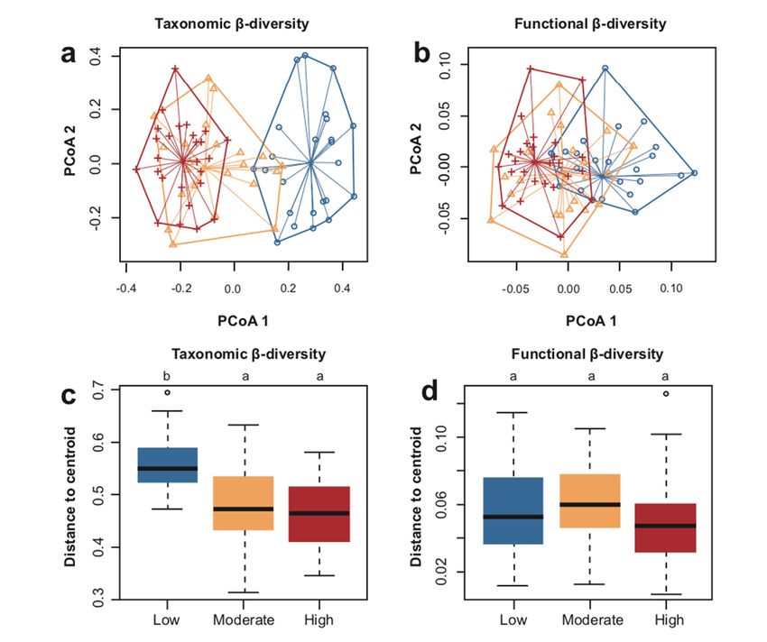
Forests 2020, 11, 1036                                                                               2 of 22

habitat degradation and biodiversity loss [9]. Habitat heterogeneity and fragmentation are considered
to be the main consequences of human disturbance [10]. With the development of built-up areas,
large natural habitats were transformed into several isolated patches with different biotic and abiotic
conditions, which affect species distribution patterns and composition by the filter on ecological
demand and dispersal ability of species [11]. Moreover, anthropogenic disturbance could induce
habitat degradation by changing soil, hydrological conditions, biogeochemical cycles, and temperature
regime, which resulted in the replacement of diverse plant assemblages by widespread, tolerant
species [11,12]. Combination of the previously mentioned factors can cause floristic dissimilarity to be
overall reduced in disturbed environments. Thus, over the past two decades, the effect of anthropogenic
disturbance on floristic homogenization has become an emerging hotspot in ecology [13–16]. Thus far,
studies on floristic homogenization have been primarily conducted by comparing the plant assemblages
at different urbanization and habitat disturbance levels [15,17–21]. However, existing studies have
achieved divergent results. Some of the studies reported a decrease in β-diversity with the increase
in anthropogenic disturbance, while others detected an increase or even no change at all [18,19,21].
In any case, species invasions and extinctions are the main causes of biotic homogenization, whilst
other habitat alterations that come with human disturbance (e.g., the habitat’s heterogeneity and
fragmentation, land-use change as well as the intensity and time span of urban sprawl) are factors
critically contributing to floristic homogenization [22,23]. However, a comparison of floristic similarity
among sites at different disturbance levels has been commonly performed after removing the effect
of environmental factors [14,18,24]. Thus far, the association of environmental factors and human
disturbance to floristic similarity has been rarely studied at a small-scale, which may hinder the
management of urban landscape and habitats.
      Though increasing studies have reported the impact of human disturbance on flora
homogenization, the emphasis of the existing studies was primarily placed on taxonomic
homogenization. However, homogenization can be also manifested in increased similarity in
the trait composition, a process known as functional homogenization, which is arousing gradual
attention [25–27]. Traits are crucial indicators to determine biodiversity as impacted by their roles of
shaping species distribution patterns [28], promoting ecosystem stability and functioning [5], as well as
determining responses to environmental changes [29]. For instance, common environmental changes
caused by human disturbance include elevated temperature, drought, and alkaline and eutrophic
soils; these changes could potentially act as biotic environmental stressors or filters, impacting plants
depending on the traits they have evolved to utilize external environments (e.g., moisture preference,
nutrition requirement, dispersal strategy, leaf traits, and lifeform) [30,31]. Since functional traits often
reflect the requirements of vegetation for the environment and show close relationships with human
disturbance [32], trait-based approaches should be conducted in combination with species-based
approaches to comprehensively study the relationship between anthropogenic disturbances and
floristic homogenization.
      Floodplain areas are one of the most significantly threatened ecosystems that exhibit susceptibility
to anthropogenic impacts [33]; research involving riparian plant assemblages may be highly conducive
to connecting local floras’ responses to degradation level with β-diversity. However, it is noteworthy
that limited studies assessing the impacts of anthropogenic disturbance on the β-diversity of plant
communities have been conducted in riparian areas [6,18,34]. Floodplain areas encompass the space
between the running water and the floodplain, where vegetation is subject to natural disturbance,
such as flooding, sediment, and inundation [35]. However, as an attraction of urbanization and human
activities, riparian areas and plant assemblages come under the pressure of artificial disturbances [36,37].
To be specific, anthropogenic disturbance in floodplain areas is associated with the expansion of
impervious surfaces, which alters hydrological and sediment regimes, increases the frequency of
flood events, and inhibits the infiltration of rainfall, thus causing natural floodplain habitats to be lost
and degraded [38,39]. On the other hand, humans impose intensive pressures on floodplain areas.
Some of the most apparent types of disturbance consist of soil compaction, water and soil pollution,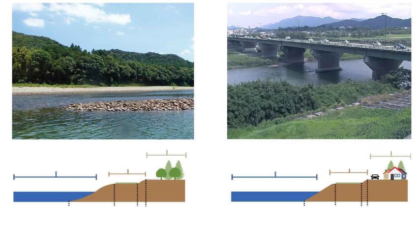
Forests 2020, 11, 1036 3 of 22
trampling of vegetation, and introduction of non-native species [40,41]. Moreover, anthropogenic
disturbance disrupts the heterogeneity of the floodplain landscape by construction of hardening banks
and recreational spaces, and destruction of floodplain forests, which in turn alters the composition
and diversity of plant assemblages [42,43]. It has been increasingly evidenced that anthropogenic
disturbance affects biodiversity, whereas most of the relevant studies have focused on residential areas
or parks [14,17,44]. Hence, it is necessary and urgent to elucidate the sustainable developing systems in
the floodplain areas to better support their ecological services (e.g., providing heterogeneous habitats
and maintaining biodiversity) [45].
Thus, this study analyzed floristic homogenization in the floodplain landscape to explore the
responses of β-diversity to the invasion of non-natives and environmental factors. The focus was on
all the shrubs and herbaceous species that occur in the sampling sites, since the previously mentioned
layers contain the majority of species richness in riparian ecosystems and exhibit the susceptibility to
environmental change [46,47]. This study aimed to understand the effects of anthropogenic disturbance
on patterns of taxonomic and functional homogenization in shrub and herbaceous assemblages in the
floodplain area. The following objectives were set: (1) to examine whether human disturbance induces
floristic homogenization, (2) to identify whether the increase in non-native species generates floristic
homogenization, and (3) to determine the effects of the environmental matrix (LULC parameters and
human disturbance) on floristic homogenization. This study predicted (1) floristic homogenization
driven by the high level of human disturbance, (2) floristic homogenization associated with increased
non-native species, and (3) the environmental matrix may affect the taxonomic and functional
β-diversity of plant assemblages.
2. Materials and Methods
2.1. Study Area
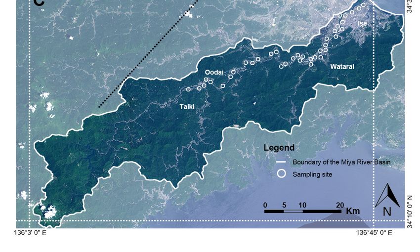
The study was conducted in the Mie Prefecture (Central Japan). We selected the floodplain area of
the Miya River for this study (Figure 1). The Miya River originates from Mt. Ōdaigahara and flows
into the Ise Bay. It is officially classified as a Class 1 river by the Japanese government and is one of
four Class 1 rivers that flow solely through Mie Prefecture. This river exhibits a 91 km length and a
basin area of approximately 920 km2 . The average annual temperature is 15 ◦ C, and the mean annual
precipitation is about 1847.8 mm (average at the Obata observation station for 2002–2018, which is
located in this study area). The Miya River basin is composed of Ise City, Tamaki Town, Watarai
Town, Taki Town, Ōdai Town, and Taiki Town. The population of this river basin is approximately
140,000, primarily concentrated in Ise City. The land-use status in the Miya River basin is nearly 84%
mountainous areas, about 8% farmland, about 4% urban (e.g., homestead), and approximately 4% other
areas (Ministry of Land, Infrastructure, Transport, and Tourism, 2016). The urban area is concentrated
in Ise City in the lower reaches. The source basin and upper reaches are designated as national parks
and county parks, respectively, and the forest area ratio is high.
The Miya River basin can be roughly split into the source part, the upper part of the mountain,
the middle part of the hill, and the lower part of the plain. Moreover, vegetation, climate, and
land-use also exhibit different characteristics according to the differences in these areas (Ministry of
Land, Infrastructure, Transport, and Tourism, 2016). The source reach is characterized by continuous
mountain areas with an average altitude of more than 500 m. Fagus crenata Blume, Tsuga sieboldii Carr.,
and Cryptomeria japonica (L.f.) D.Don are the dominant species, forming a forest landscape. The upper
reach winds its way through the V-shaped valley in the low mountains, achieving an average altitude
range of 100–500 m. The riparian areas in the middle reach are formed in the hills, with an average
altitude of approximately 300 m. The middle reach of the Miya River is narrow and composed of a
continuous forested strip, gravel floodplain, and cultivated areas. The dominant plant species include
Chamaecyparis obtuse (Siebold & Zucc.) Endl. and Cryptomeria japonica. The lower reach with an altitude
below 100 m above sea level is characterized by vast agricultural landscapes and the core urban area of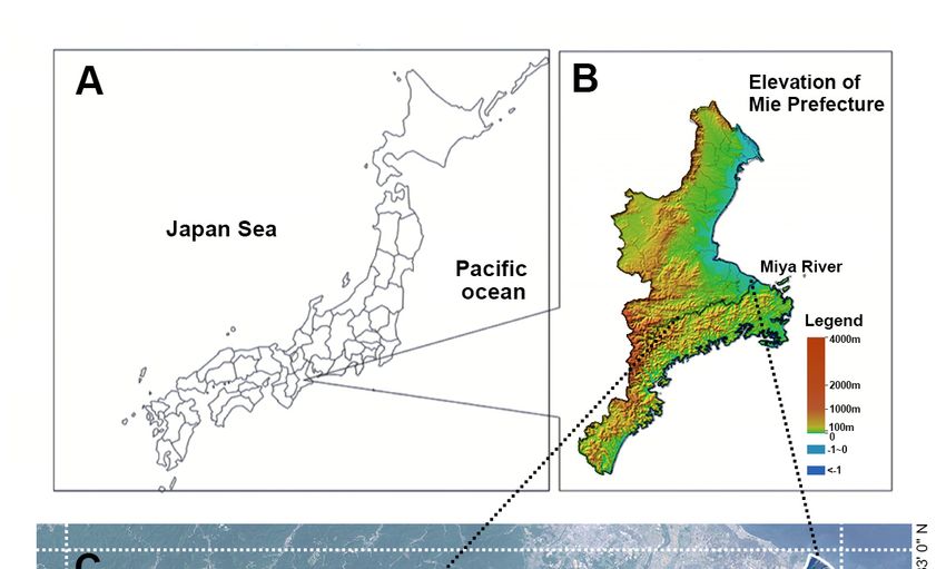
Forests 2020, 11, 1036                                                                                    4 of 22

Forests 2020, 11, x FOR PEER REVIEW                                                                      4 of 23
 Ise City. In the lower reach area, the floodplain has been frequently employed as a recreational space.
floodplain
 Moreover,area    in the residents
             to protect  lower reach  hasflooding,
                                   from    been reinforced. Thefloodplain
                                                   most of the   plant species
                                                                          areathat dominated
                                                                               in the          in this
                                                                                      lower reach  has area
                                                                                                       been
were  Phragmites    australis (Cav.)  Trin. ex Steud. and Phragmites   japonica Steud.
 reinforced. The plant species that dominated in this area were Phragmites australis (Cav.) Trin. ex Steud.
 and Phragmites japonica Steud.

       Figure 1. (A) Location of the Mie Prefecture. (B) Location of the Miya River and elevation map of the
       Mie Prefecture.
      Figure           (C) Area
             1. (A) Location     of the
                             of the MieMiya  River basin
                                        Prefecture.      and the of
                                                    (B) Location location of sampling
                                                                    the Miya  River andplots.
                                                                                        elevation map of the
      Mie Prefecture. (C) Area of the Miya River basin and the location of sampling plots.
 2.2. Field Sampling
2.2. Field Sampling
       Ideally, the extant and historical vegetation data should be used to compare the effect of
 anthropogenic disturbance on the variation of floras. Since these data are usually unavailable, sampling
      Ideally, the extant and historical vegetation data should be used to compare the effect of
 sites with different degradation levels are commonly compared to determine a spatial change in plant
anthropogenic disturbance on the variation of floras. Since these data are usually unavailable,
 communities. Therefore, this approach was applied in the present study. First of all, the lower, middle,
sampling sites with different degradation levels are commonly compared to determine a spatial
change in plant communities. Therefore, this approach was applied in the present study. First of all,
the lower, middle, and upper reaches of the Miya River basin were selected as the study area, because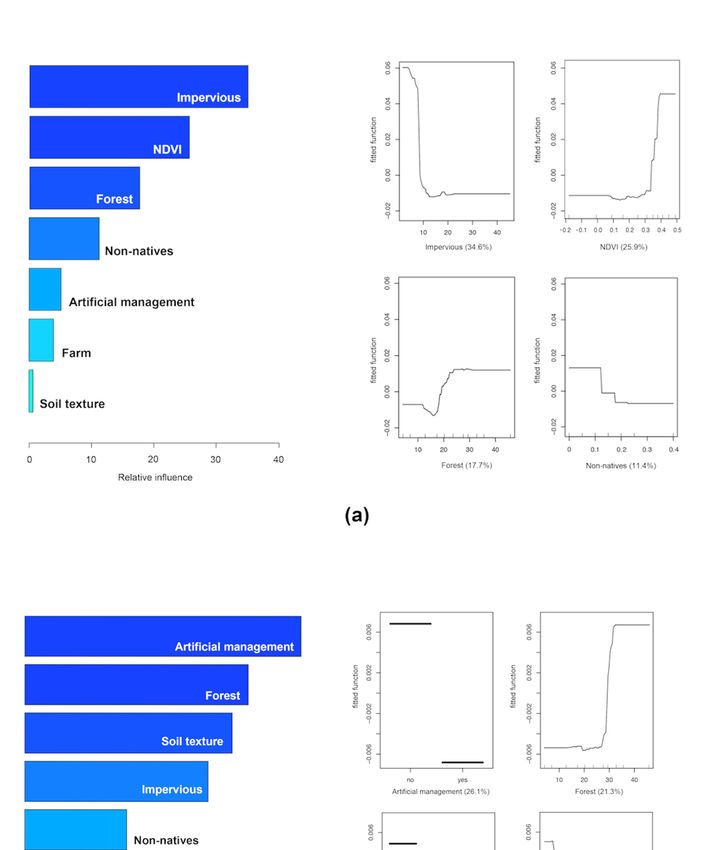
Forests 2020, 11, 1036 5 of 22
and upper
Forests reaches
2020, 11, of theREVIEW
x FOR PEER Miya River basin were selected as the study area, because these areas can5reflect
of 22
the variation of anthropogenic disturbance. The lower reach of the Miya River is located within Ise City,
subject to
middle andtheupper
modification
reaches ofof riparian
the Miya land cover
River areand human activities.
embellished by paddy The middle
fields, teaand upper
fields, reaches
as well as
of the Miya
peasant River are Secondly,
households. embellished to by paddy
obtain fields, tea
unbiased andfields, as well
spatially as peasant households.
well-represented samplingSecondly,
sites, a
to obtaindigital
1/25,000 unbiasedlandand spatially
condition mapwell-represented sampling sites,
(geospatial information a 1/25,000
authority digital
of Japan, land
2014) condition
was used asmapthe
(geospatial
base information
layer, and the basinauthority
area wasofdivided
Japan, 2014)
into 74 was used as
squares the an
with base layer,
area and the
of 1km 2 basin
(each area was
square was
divided intoas
considered 74asquares
potential an area of 1km2of(each
withrepresentation square was
a sampling considered
site). as a potential
The sampling representation
sites were selected
of a sampling
according site). condition
to land The sampling sites were
(riparian selected
lowland), according
size (floodplainto land
widthcondition
>50 m), (riparian lowland),
and vegetation
size (floodplain
structure width
(vegetation >50>80%
cover m), and andvegetation
excluded barestructure (vegetation
ground). In this step, the>80%
cover andimage
satellite excluded bare
(1:5000),
ground). In this step, the satellite image (1:5000), and 1/25,000 vegetation
and 1/25,000 vegetation map downloaded from J-IBIS (Japan Integrated Biodiversity Information map downloaded from
J-IBIS (Japan
System, 2013; Integrated Biodiversity Information System,
https://www.biodic.go.jp/index.html) 2013;as
were used https://www.biodic.go.jp/index.html)
Supplementary Materials. Then, a
wereof
total used as Supplementary
49 floodplain areas were Materials.
selectedThen, a totalto
according ofpreviously
49 floodplain areas were
mentioned selected
criteria. accordingto
Meanwhile, to
previously mentioned criteria. Meanwhile, to eliminate the influence of inaccessibility
eliminate the influence of inaccessibility and significant differences in environmental conditions, we and significant
differencesain
conducted environmental
field reconnaissance conditions,
survey towe conducted
ensure a field reconnaissance
the appropriateness of the 49 survey to ensure
floodplains. the
Finally,
appropriateness
36 sampling sites of the 49 floodplains.
were selected from Finally, 36 sampling
the upper sites were
to lower selected
reaches. Amongfromthe the 13
upper to lower
eliminated
reaches. Among
floodplains, the 13 eliminated
9 floodplains floodplains,
were forbidden 9 floodplains
to access were forbidden
and 4 floodplains weretoexcluded
access and for4inadequate
floodplains
were excluded
vegetation for inadequate
coverage. In some parts vegetation coverage. areas,
of the floodplain In some parts lowlands
riparian of the floodplain areas, riparian
were transformed into
lowlands were transformed into major beds, thus major beds and waterside
major beds, thus major beds and waterside lowlands of the floodplain area were selected as the lowlands of the floodplain
area were
primary selectedarea
sampling as the primary
(Figure 2). sampling area (Figure 2).
a b
c Uplands
d Uplands
Floodplain Floodplain
Body of Water Body of Water
Edge of the Waterside Natural Edge of the Major Bed Bank
Lowland Lowland Slope Major Bed Slope
Figure 2. Examples of the sampling area. (a,b) example images of waterside lowland and major bed;
Figure 2. Examples of the sampling area. (a,b) example images of waterside lowland and major bed;
(c,d) example section structure of waterside lowland and major bed.
(c,d) example section structure of waterside lowland and major bed.
A vegetation survey was carried out by using the line transect method [48]. In each of the selected
A vegetation
sampling survey
sites, 10 × was carried
10 m sampling outwere
plots by using the line
positioned transect
along transectsmethod [48]. In each
perpendicular to theofriver
the
selected sampling
at intervals sites,m.10According
of 50–100 × 10 m sampling plots were
to the length of thepositioned
shore, each along transects
sampling site perpendicular
contained one to or
the
two transects, aiming to establish the effort of transects proportionate to floodplain site
river at intervals of 50–100 m. According to the length of the shore, each sampling contained
length. When
one or two of
the length transects, aiming
the sampling to establish
areas was not the efforttoofaccommodate
enough transects proportionate to floodplain
the two transects, length.
two sampling
When the length of the sampling areas was not enough to accommodate the
plots were established along the transect to ensure that each sampling site had two sampling plots. two transects, two
sampling plots were established along the transect to ensure that each
The shrubs were recorded in the 10 × 10 m plots, and the herbs and grasses were investigated in sampling site had two
sampling plots.ofThe
5 smaller plots 1 × shrubs
1 m, and were recorded
randomly in the
nested 10 10
in the × 10 mm
× 10 plots,
plot.and the herbs
In each and
plot, the grasses
name, were
coverage,
investigated in 5 smaller plots of 1 × 1 m, and randomly nested in the 10 × 10 m
and density of all shrubs and herbs were measured. The coverage of each plant was measured visually plot. In each plot, the
name, coverage, and density of all shrubs and herbs were measured. The coverage
within each sampling plot according to a scale of 1–5: 1 = less than 5%, 2 = 5%–25%, 3 = 25%–50%, of each plant was
measured
4 = 50%–75%,visually within each
5 = 75%–100% sampling
[49]. plot according
The density to a scale
of plant species was of 1–5: 1 =byless
recorded than 5%,
counting the2number
= 5%–
25%, 3 = 25%–50%, 4 = 50%–75%, 5 = 75%–100% [49]. The density of plant species was recorded by
counting the number of individuals within a range of 1 × 1 m. Regarding clonal species, which have
many stems for each individual, density was determined by dividing the total stem number by the
mean number of stems per individual. Although tree species were recorded in the investigation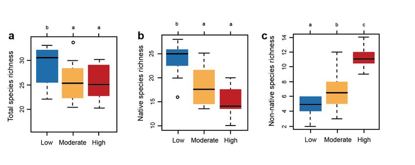
Forests 2020, 11, 1036                                                                                    6 of 22

of individuals within a range of 1 × 1 m. Regarding clonal species, which have many stems for
each individual, density was determined by dividing the total stem number by the mean number of
stems per individual. Although tree species were recorded in the investigation process, they were
excluded from further analyses for two reasons: (1) herbaceous and woody species respond differently
to environmental change for the differences in turnover rate and longevity, therefore, adding tree data
in vegetation analysis might lead to an inaccurate result in the current study; (2) trees in our study area
may have an artificial character and there was no information available to distinguish planted trees
from natural occurrences, thus the information that was involved in forest stand and management
was not considered as an anthropogenic predictor for environment vegetation analysis. Plant species
were identified to the species level in situ. For those species that could not be immediately identified,
specimens were taken to the laboratory where they were identified by matching with a botanical guide
and preserved herbarium specimens. Five soil samples were collected from five small plots that were
randomly selected in each sampling plot at a depth of 0–40 cm to determine the soil texture. All soil
samples were removed with a corer and were stored in labeled plastic bags immediately afterward.

2.3. Delineation of Sampling Area into Different Level of Habitat Degradation
      The level of habitat degradation was delineated by calculating the Normalized Difference
Vegetation Index (NDVI) [50] (Supplementary A). A 500-m buffer zone was set around each sampling
site to calculate the NDVI. This index could be calculated by measuring the difference in reflectance
between the red band (RED) and near-infrared band (NIR) of the satellite images. The NDVI ranges
from −1.0 to +1.0, where positive values represent the increase in the amounts of green vegetation and
negative values indicate the degradation of the habitat [51]. The NDVI was calculated by:

                                                       NIR − RED
                                            NDVI =                                                            (1)
                                                       NIR + RED

where NIR denotes the near-infrared band digital number value; RED is the red band digital number
value. The NDVI was calculated based on a Landsat ETM 7 satellite image (30-m resolution;
https://glovis.usgs.gov, accessed 16 September 2019) with ArcGIS 10.2 software (ESRI, 2013, Redlands,
CA, USA). The NDVI values of all sampling plots in the surrounding buffer zone were averaged.
k-means clustering based on mean NDVI values was used to classify floodplains into different levels
of habitat degradation—high, moderate, and low (Table 1). The NDVI was correlated with plant
photosynthetic activity and was adopted as an indicator of habitat degradation, since NDVI values in
highly disturbed areas are smaller than those in less disturbed areas [52,53]. Furthermore, the NDVI
was reported to be a powerful proxy and screening tool for monitoring and assessment of riparian
habitats [54].

      Table 1. Number and location of floodplain areas selected at different degradation levels. Notes: the
      information of the population was derived from the Mie Prefectural Government.

          Characteristic                 High                    Moderate                     Low
     Number of floodplains                13                         11                        12
      Mean NDVI values                −0.11–0.17                  0.17–0.4                  0.4–0.58
                                       Ise City
                                                              Watarai Cho area,      Taiki Cho area, Ōdai
                                (Miyagawatutumi Park,
     Location of floodplains                                 Tsumura Cho area,      Town, Kawazoe station
                                   Love River Park,
                                                              Souchi Cho area                area
                                Miyagawashinsui Park)
          Proportion of
                                         25.47                     12.97                      5.31
     impervious surface (%)
       Human population                  96,387                    15,439                    11,603
      Total number of plots                26                        22                        24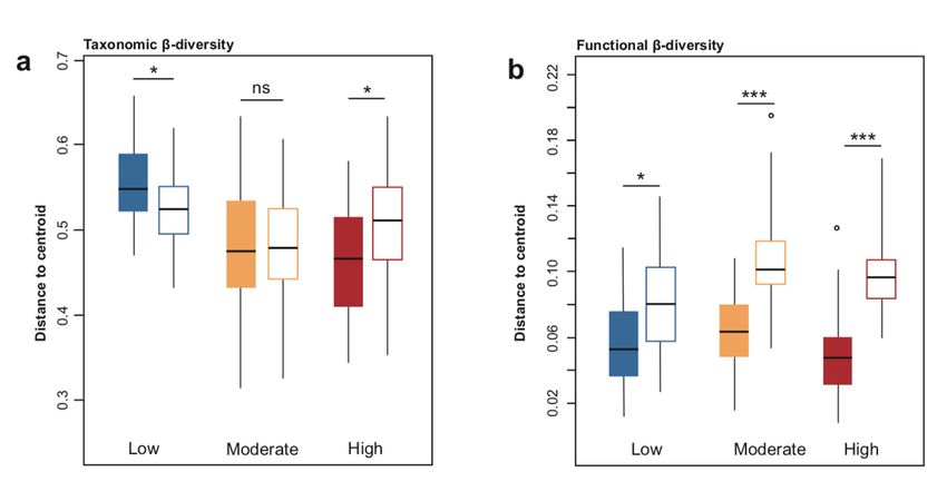
Forests 2020, 11, 1036                                                                                           7 of 22

2.4. Functional Traits
      Each plant species was identified as seven reproductive, physiological, and morphological trait
groups. These functional traits could be adopted to measure the impact of environmental change
and to quantify the effect of plant assemblages shift on ecosystem processes. Moreover, several
environmental indices (Table 2) were select for their representativeness as responses to natural and
anthropogenic disturbances [31]. The plant height was measured in situ. Subsequently, the height
data were transformed into five ordinal groups by performing a k-means clustering. Moreover,
several surrogate traits were used to assess the ability of plant species to tolerate anthropogenic and
hydrological disturbances [32]. For example, the wetness level was adopted as an indicator for the
ability of plant species to address alteration of hydrological regimes, so it was linked to the probability
of a plant species occurring in floodplain habitats. Shade tolerance is a crucial functional trait that
significantly impacts plant community dynamics and is closely correlated with numerous plant traits
(e.g., specific leaf area and photosynthetic rate) [55]. Shade tolerance was characterized since it can
reflect the forest structure and dynamics in the floodplain area. On the other hand, shade tolerance
could reflect the light demand of plant species since light intensity was closely related to human
disturbance [56]. Fertility requirement was considered for high nutrition environments and is related
closely to the disturbed area [31]. The approach of seed dispersal could indirectly reflect the effect of
habitat fragmentation and human disturbance, thus it was included in this study [9]. The data of plant
traits were acquired from the field measurements and available published data (see Supplementary B
for further details). Considering that the trait values retrieved from the database may be inaccurate,
qualitative values instead of quantitative values were adopted to minimize the deviations attributed to
the use of trait databases.

      Table 2. Ten trait groups and trait states use in the trait matrix. The sources of literature were listed in
      Supplementary B.

                   Trait                                           Trait State
                 Life form                       Annual forb; Perennial forb; Shrub; Fern
               Height (cm)                    1–50; 51–100; 101–150; 151–200; More than 200
             Reproduction                          Vegetative; Vegetative and seed; Seed
            Shade tolerance                          Intolerant; Mid-tolerant; Tolerant
              Wetness level        Upland; Facultative upland; Facultative; Facultative riparian; Riparian
               Growth rate                                Rapid; Moderate; Slow
                Seed bank                                   Transient; Persistent
            Seed abundance                                  High; Medium; Low
          Fertility requirement                             High; Medium; Low
             Seed dispersal                       Wind; Water/gravity; animal, multiple

2.5. Land-Use (Land Cover) and Habitat Data
     Given the differences in LULC distribution and combination activities existing among three
groups of degradation levels [15], the proportions of various land-use types in the surroundings
of the sampling plots were extracted to assess the effect of the anthropogenic factors on floodplain
floras. To be specific, three predominant land-use types in the studied floodplain landscape were
identified, which consisted of (1) impervious surface (rigid pavement area, i.e., buildings, pavement,
and roads), (2) forest, and (3) farmland. Different land-use types were delineated in a 500 m radius
circular buffer zone around each sampling plot, with Google Earth imagery (2019) as a base layer.
To interpret the surrounding land-use type of each sampling plot, we used feature-extraction techniques
with ArcGIS 10.2 software (ESRI, 2013, Redlands, CA, USA). In this classification processing step,
aerial photograph interpretation and ground features are crucial in providing reference information
for each land-use class [57]. Moreover, the management method of floodplains and soil texture
was used. Artificial construction was considered as a predictor of degradation of the riparian area,
as the construction altered the sediment regimes and hydrological conditions, and added intense
Forests 2020, 11, 1036 8 of 22
human recreational activities [58]. Soil texture was used as an environmental factor related to local
environmental conditions [59]. Coarse-textured floodplain soil displayed a constant link to intensive
flush flooding. Soil texture was identified as silt (2 mm)
using a Malvern Mastersizer 3000 (Malvern Panalytical Ltd., Malvern, UK).
2.6. Statistical Analysis
2.6.1. α- and β-Diversity
The species α diversity was quantified by species richness. Species richness was determined by
counting the number of species in plant communities at the plot scale. Furthermore, one-way analysis
of variance (ANOVA) was conducted by the least significant difference (LSD) test.
To investigate the variation of species and plant traits in plant assemblages, the taxonomic and
functional β-diversity across the river basin were calculated. The β-diversity here denoted the total
β-diversity (dissimilarity among all the sampling plots), which was assessed by the Bray–Curtis
dissimilarity [60]. The Bray–Curtis dissimilarity ranged from 0 to 1, where 0 meant that the two plots
had the same composition, and 1 meant that the two plots did not share any species or functional groups.
To delve into the effect of anthropogenic disturbance on floristic homogenization, taxonomic
and functional facets were calculated following three steps. First, a functional matrix was built by
multiplying the species-by-trait matrix with the plot-by-species matrix. For the plot-by-species matrix,
we used species relative abundance data to measure the dominance of a species on each sampling plot.
Second, for an in-depth analysis, the species matrix and the functional matrix should be transformed
into a plot-by-plot distance matrix. For taxonomic β-diversity, the Bray–Curtis distance on the
plot-by-species matrix was employed to generate the plot-by-plot distance matrix. For functional
β-diversity, the plot-by-plot distance matrix was computed on the plot-by-trait using the Gower distance.
Third, we tested whether anthropogenic disturbance was responsible for floristic homogenization
by the approach of Test for Homogeneity of Multivariate Dispersions [61]. This test could analyze
the β-diversity (the distance of each site to their group centroid) based on the plot-by-plot distance
matrix and subject the acquired values to permutation tests to verify whether these distances differed
among groups. Then, we tested the site distances to centroid using ANOVA with 9999 permutations
to determine whether the dispersion of three groups of degradation levels differed. Furthermore,
the differences in the variations in taxonomic and functional compositions (location differences
between centroids) were tested using PERMANOVA [62], and the significance was assessed using
9999 permutations with pseudo-F ratios. The differences in taxonomic and functional multivariate
dispersion and composition among three groups of degradation levels were visualized by Principal
Coordinate Analysis (PCoA).
2.6.2. Effect of Increase of Non-Native Species
The effect of non-native species on floristic homogenization could be measured by the variations
of β-diversity. Thus, the β-diversity (site distance to the centroid) for all plant species was compared to
that for natives only. This approach could simulate the invasion of non-natives in a plant community
by comparing the changes of β-diversity after “adding” them; on that basis, whether they lead to
homogenization can be evaluated. The native β-diversity was compared to that of all species by paired
sample t-tests, and p-values were adjusted by the multiple test Holm correction.
2.6.3. Effect of Environmental Matrix on β-Diversity
The entire set of predictor variables consisted of the proportion of impervious surface,
the proportion of forest, proportion of farmland, management method of floodplains, soil texture,
as well as the dominance of non-native species (the sum of relative abundance of the non-native species
in each plot). First, these predictors were subjected to one-way ANOVA to determine the differences
among degradation groups. Correlation analysis (Pearson r) was first performed among the predictorsForests
Forests 2020,2020, 11, x FOR PEER REVIEW
11, 1036 9 of922
of 22
species was correlated with the proportion of impervious surface (r = 0.48). Since the joint effects of
to determine
non-natives theand
multicollinearity
environmentalinfactors our models. We found
on β-diversity the dominance
should be determined of non-native
and the rspecies wasless
value was
correlated with the proportion of impervious surface (r = 0.48). Since the joint
than 0.7, all the predictors were kept. With the total β-diversity of sample plots as the response,effects of non-natives and we
environmental
performed boostedfactors on β-diversity
regression tree should
analysisbe determined
(BRT) and thethe
[63] to analyze r value
effectwas less than 0.7, all
of environmental the
variables
predictors were kept. With the total β-diversity of sample plots as the response,
on taxonomic and functional β-diversity. BRT was used for its good interpretability and its flexibilitywe performed boosted
regression tree analysis
in handling different(BRT)
types[63] to analyzeand
of predictors the effect of environmental
less sensitivity variables on[64].
to multicollinearity taxonomic and the
BRT ranks
functional significanceBRT
relativeβ-diversity. andwas used for
displays theits good interpretability
individual effects of each andvariable
its flexibility in handling
in a partial different
dependence plot.
types of predictors and less sensitivity to multicollinearity [64]. BRT ranks the
The proportion of forest was included since forest is a crucial component in the floodplain area andrelative significance and
displays
forestthe individual
could be used effects of each responsible
as a predictor variable in afor
partial dependence
floristic plot. Thewhere
homogenization, proportion of forest
plots with a large
wascover
included since forest
of forest, is a crucial
in general, component
also have in the floodplain
high diversity. The BRTarea model andwasforest could be used
performed usingasa atree
predictor responsible
complexity of five,for floristic homogenization,
a learning rate of 0.001, and where plots with
a bag fraction a large cover of forest, in general,
of 0.5.
also haveAll high diversity.
statistical The BRT
analyses thatmodel was performed
we applied here were using a tree complexity
implemented of five,3.2.2.
in R version a learning rate
The k-means
of 0.001, and a bag fraction of 0.5.
cluster analyses, Pearson correlation analysis, and LSD tests in ANOVA were performed with the
All package.
stats statisticalTheanalyses that we
functional traitapplied hereimplemented
matrix was were implemented in R package
in the “fd” version 3.2.2. The“functcomp”
with the k-means
cluster analyses,
function Pearson
[65]. The correlation
multivariate analysis,
dispersion and LSD
analyses weretests in ANOVA
performed were
in the performed
“vegan” with
package the the
with
stats package. The functional trait matrix was implemented in the “fd” package
“betadisper” function [66]. The comparisons of the distance of each plot to the centroid were drawn with the “functcomp”
function
with the[65].“permutest.betadisper”,
The multivariate dispersion and analyses were performed
the comparisons of locationin theusing
“vegan” package
“rda” with the
and “anova.cca”
“betadisper”
(vegan) were function [66]. The
conducted. Thecomparisons of the distance
BRTs were adopted using theof each
code plotfromtothe the‘gbm’
centroid were drawn
incorporated in the
with the “permutest.betadisper”,
“dismo” package [67]. and the comparisons of location using “rda” and “anova.cca” (vegan)
were conducted. The BRTs were adopted using the code from the ‘gbm’ incorporated in the “dismo”
3. Results
package [67].
3. Results
3.1. Species Richness and Composition of Plant Assemblages
A total
3.1. Species of 124
Richness andspecies were of
Composition found
Plantacross all study sites, 37 of which were non-native species.
Assemblages
Significant differences were identified between different degradation levels for total, native, and non-
A total of 124 species were found across all study sites, 37 of which were non-native
native species richness (Figure 3). The total species richness was significantly higher at the low
species. Significant differences were identified between different degradation levels for total, native,
degradation level than moderate and high degradation levels; the species richness of non-natives was
and non-native species richness (Figure 3). The total species richness was significantly higher at the
significantly higher in highly disturbed areas and reached its lowest value at the low degradation
low degradation level than moderate and high degradation levels; the species richness of non-natives
level. The species richness of natives was significantly higher at the low degradation level than that
was significantly higher in highly disturbed areas and reached its lowest value at the low degradation
in the moderate and high degradation levels.
level. The species richness of natives was significantly higher at the low degradation level than that in
the moderate and high degradation levels.
Figure 3. Total species richness (a), native species richness (b), and non-native species richness (c) in
different levels of degradation. Data provided show the median (bold line), 25%–75% quartiles (boxes),
Figure 3. Total species richness (a), native species richness (b), and non-native species richness (c) in
ranges (whiskers), and outliers (white dot). Significant differences are presented by different letters
different levels of degradation. Data provided show the median (bold line), 25%–75% quartiles
(p < 0.05).
(boxes), ranges (whiskers), and outliers (white dot). Significant differences are presented by different
letters (pthe
Regarding < 0.05).
most frequent species found in the floodplain area, six native species represent the
widespread common species that were observed in most plots throughout the study area. Besides,
Regarding
four non-native the most
species werefrequent
includedspecies
in thefound in most
top ten the floodplain area, species
frequent plant six native species
(Table 3). represent
These
the widespread common species that were observed in most plots throughout the study area.
non-native species were recorded at high frequency (more than 41.7%) at high and moderate degradation Besides,
four non-native species were included in the top ten most frequent plant species (Table 3). These non-Forests 2020, 11, 1036 10 of 22
levels, whereas there was a relatively low frequency (less than 20.8%) of non-natives observed in areas
at the low degradation level. Riparian plant species, such as Miscanthus sacchariflorus (Maxim.) Franch.
and Phragmites japonica, were recorded with a higher frequency in areas at the low degradation level
than those in highly disturbed areas.
Table 3. The top 10 most frequent plant species found in floodplain area. Plant species were ranked
by frequency of occurrence in all sampling plots (n = 72 plots). Notes: species in bold indicate
non-native species.
Family Species High (%) Moderate (%) Low (%)
Polygonaceae Rumex acetosa (L.) 66.7 54.2 58.3
Artemisia indica Willd. var.
Asteraceae 75 70.8 25.0
maximowiczii (Nakai)H. Hara
Asteraceae Solidago altissima (L.) 79.2 70.8 4.2
Asteraceae Erigeron annuus (L.) Pers. 83.3 41.7 8.3
Poaceae Lolium multiflorum Lam. 50.0 58.3 20.8
Rosaceae Rosa multiflora Thunb. 58.3 33.3 37.5
Poaceae Miscanthus sacchariflorus 37.5 41.7 45.8
Fabaceae Trifolium repens (L.) 54.2 50 20.8
Poaceae Phragmites japonica 25 37.5 41.7
Poaceae Festuca arundinacea Scherb. 50 37.5 8.3
3.2. Taxonomic and Functional β-Diversity
For the taxonomic aspect, the β-diversity differed significantly with different degradation levels
(significant multivariate dispersion tests; Table 4). The dissimilarity was lower at high degradation levels
than that at low levels (see polygon size on Figure 4a; and average sites-to-centroid distance illustrated
in Figure 4c), indicating that a relatively high degradation level caused taxonomic homogenization.
For the functional aspect, however, homogenization phenomenon was absent in degradation levels.
Though the β-diversity was lower in highly disturbed areas compared with the areas at moderate and
low degradation levels (Figure 4b,d), the differences were not significant by significant multivariate
dispersion tests (Table 4).
β-diversity changes were associated with the species and trait composition among degradation
levels. The PERMANOVA revealed significant shifts in taxonomic and functional compositions
(centroid location) for both taxonomic and functional β-diversity (Table 4), as represented by the
isolated location of the centroid at a low degradation level relative to that at high and moderate
degradation levels (Figure 4). As revealed from the differences in the location of the centroid, species
and traits diverged between the low degradation level and the other two types of degradation
levels. However, the relatively short distance between centroids at high and moderate degradation
levels showed that the shifts in species and traits composition were similar in these two types of
degradation levels.
Table 4. Differences in β-diversity and composition in the floodplain landscape, according to three
groups of degradation levels. Note: difference in β-diversity was tested with ANOVA by permutations
on site–centroids distances and difference in location of centroid was tested with PERMANOVA.
Taxonomic Aspect Functional Aspect
F Ratio p-Value F Ratio p-Value
β-diversity 16.92Forests2020,
Forests 11,x1036
2020,11, FOR PEER REVIEW 1111ofof22
22
Figure 4. Effect of different degradation levels on the multivariate dispersion of species (a,c) and
Figure 4. Effect of different degradation levels on the multivariate dispersion of species (a,c) and trait
trait (b,d) composition in floodplain landscape. Taxonomic and functional β-diversity is measured
(b,d) composition in floodplain landscape. Taxonomic and functional β-diversity is measured as the
as the distance of sites to their group centroid (using Bray–Curtis and Gower distances, respectively),
distance of sites to their group centroid (using Bray–Curtis and Gower distances, respectively), here
here represented on the first two axes of a PCoA and using a boxplot (median and quartiles) of the
represented on the first two axes of a PCoA and using a boxplot (median and quartiles) of the sites-
sites-to-centroid distance. On the PCoA, a change in site dispersion around the centroid represents
to-centroid distance. On the PCoA, a change in site dispersion around the centroid represents a
a change in β-diversity, while a change in the centroid location represents a species/trait turnover.
change in β-diversity, while a change in the centroid location represents a species/trait turnover.
Symbols represent each plot in different degradation levels: + = high, ∆ = moderate, and # = low.
Symbols represent
Values share each plot
same letter in different
are not degradation
significantly levels:
different at + = high, ∆ level.
0.05 significance = moderate, and ○ = low.
Values share same letter are not significantly different at 0.05 significance level.
3.3. The Role of Non-Native Species in β-Diversity
Table 4. Differences in β-diversity and composition in the floodplain landscape, according to three
In the taxonomic and functional aspects of the flora, the results of this study showed that
groups of degradation levels. Note: difference in β-diversity was tested with ANOVA by
the invasion of non-native species in native plant assemblages drives different variation patterns
permutations on site–centroids distances and difference in location of centroid was tested with
of β-diversity (Figure 5, Supplementary C). The homogenization effect was significant at a high
PERMANOVA.
degradation level both in taxonomic and functional aspects after the Holm correction. The increase in
Taxonomic
non-native species at the moderate degradation levelAspect Functional
improved Aspect only in functional
homogenization
F Ratio p-Value F Ratio p-Value
aspects, while the change of β-diversity in taxonomic aspects was slight. At the low degradation level,
β-diversity
the increase in non-native 16.92 a slight
species indeed causedForests 2020, 11, x FOR PEER REVIEW 12 of 22
aspects, while the change of β-diversity in taxonomic aspects was slight. At the low degradation level,
the increase in non-native species indeed caused a slight taxonomic differentiation, while it did cause
a slight homogenization in functional aspect.
Forests 2020, 11, 1036 12 of 22
Figure 5. Differences in taxonomic (a) and functional (b) β-diversity induced by non-native species in
three
Figure groups of degradation
5. Differences level. Variations
in taxonomic in β-diversity
(a) and functional were assessed
(b) β-diversity by comparing
induced by non-nativethe species
distancesin
of sites to centroids of native species (native plant species that recorded in all sampling
three groups of degradation level. Variations in β-diversity were assessed by comparing the distances plots) to those
of
of the
sitestotal flora (complete
to centroids plant
of native species
species that are
(native recorded
plant speciesin all recorded
that samplingin plots). Notes: the
all sampling color-filled
plots) to those
boxes represent the β-diversity of total species, and the color-outlined boxes represent the
of the total flora (complete plant species that are recorded in all sampling plots). Notes: the color-filled β-diversity
of native
boxes species.the
represent Asterisks indicate
β-diversity a significant
of total species, andchange in paired sample
the color-outlined boxest-tests that are
represent theadjusted by
β-diversity
the multiple test Holm correction. Significance levels: * p < 0.05; *** p < 0.001; ns, not significant.
of native species. Asterisks indicate a significant change in paired sample t-tests that are adjusted by
the multiple test Holm correction. Significance levels: * p < 0.05; *** p< 0.001; ns, not significant.
3.4. Joint Effects of Non-Native Species and Environmental Matrix
The predictor
3.4. Joint variables are
Effects of Non-Native shown
Species andin Table 5. The Matrix
Environmental results of the BRT model reflected the direct
or indirect effects of environmental factors on β-diversity. In our study, the BRT model had greater
The predictor variables are shown in Table 5. The results of the BRT model reflected the direct
predictive power on functional β-diversity (explained deviance: 0.481) than that on taxonomic
or indirect effects of environmental factors on β-diversity. In our study, the BRT model had greater
β-diversity (explained deviance: 0.429), and the relative contribution of the predictors varied between
predictive power on functional β-diversity (explained deviance: 0.481) than that on taxonomic β-
these two diversity aspects (Figure 6).
diversity (explained deviance: 0.429), and the relative contribution of the predictors varied between
The proportion of impervious surfaces had the strongest influence on the taxonomic β-diversity
these two diversity aspects (Figure 6).
in sampling plots (explaining 34.6% of the variability in taxonomic β-diversity patterns). Taxonomic
The proportion of impervious surfaces had the strongest influence on the taxonomic β-diversity
β-diversity strongly decreased between 10% and 20% of impervious surfaces, implied a relative
in sampling plots (explaining 34.6% of the variability in taxonomic β-diversity patterns). Taxonomic
small proportion of impervious surface sustains higher taxonomic β-diversity. The NDVI also had
β-diversity strongly decreased between 10% and 20% of impervious surfaces, implied a relative small
a significant effect on taxonomic β-diversity and explained 25.9% of the variation of taxonomic
proportion of impervious surface sustains higher taxonomic β-diversity. The NDVI also had a
β-diversity. The percentage of forest also critically impacted the shaping of taxonomic β-diversity
significant effect on taxonomic β-diversity and explained 25.9% of the variation of taxonomic β-
(explaining 17.7% of the variability in taxonomic β-diversity patterns), and taxonomic β-diversity
diversity. The percentage of forest also critically impacted the shaping of taxonomic β-diversity
significantly increased beyond approximately 20% of forest cover. The dominance of non-native
(explaining 17.7% of the variability in taxonomic β-diversity patterns), and taxonomic β-diversity
species was also an important predictor of taxonomic β-diversity and explained 11.4% of the variability
significantly increased beyond approximately 20% of forest cover. The dominance of non-native
in taxonomic β-diversity. For functional β-diversity, artificial management was the top predictor
species was also an important predictor of taxonomic β-diversity and explained 11.4% of the
(explaining 26.1% of the variability in functional β-diversity patterns). Partial dependency plots
variability in taxonomic β-diversity. For functional β-diversity, artificial management was the top
showed that the functional β-diversity was higher in natural floodplains than in floodplains that
predictor (explaining 26.1% of the variability in functional β-diversity patterns). Partial dependency
have been artificially transformed. Besides, functional β-diversity was also strongly explained by
plots showed that the functional β-diversity was higher in natural floodplains than in floodplains
the percentage of forest and significantly increased between 20% and 30% of the percentage of forest.
that have been artificially transformed. Besides, functional β-diversity was also strongly explained
In addition, soil texture and the proportion of impervious surface showed strong explanatory effects
by the percentage of forest and significantly increased between 20% and 30% of the percentage of
on functional β-diversity and explained 19.7% and 17.4% of the variability, respectively. For both
forest. In addition, soil texture and the proportion of impervious surface showed strong explanatory
taxonomic and functional β-diversity, the effect of the percentage of farmland was negligible.
effects on functional β-diversity and explained 19.7% and 17.4% of the variability, respectively. For
both taxonomic and functional β-diversity, the effect of the percentage of farmland was negligible.Forests 2020, 11, x FOR PEER REVIEW 13 of 22
Forests 2020, 11, 1036 13 of 22
Figure 6. Relative influence of predictors and partial dependency plots for boosted regression tree
analyses on6.taxonomic
Figure (a) and functional
Relative influence (b) and
of predictors β-diversity. For taxonomic
partial dependency for boostedexplained
plotsβ-diversity, regressiondeviance:
tree
0.429; For functional
analyses on taxonomic (a) andexplained
β-diversity, functional deviance: 0.481.For
(b) β-diversity. Numbers enclosed
taxonomic insideexplained
β-diversity, parenthesis
indicated the relative importance of predictors. Notes: forest, proportion of forest cover in a 500-m
buffer zone; impervious, proportion of impervious surface in a 500-m buffer zone, farm, proportion of
farmland in a 500-m buffer zone; non-natives, the dominance of non-native species; NDVI; mean NDVI
value in a 500-m buffer zone.Forests 2020, 11, 1036 14 of 22
Table 5. Environmental variables in three groups of degradation level. Values represent means ± SE.
Values that share the same letter are not significantly different at 0.05 significance level. Notes: forest,
proportion of forest cover in a 500-m buffer zone; impervious, proportion of impervious surface in a
500-m buffer zone, farm, proportion of farmland in a 500-m buffer zone; gravel, percentage of gravel
content; sand, percentage of sand content; silt; percentage of silt content; non-natives, the dominance of
non-native species (range from 0 to 1); artificial management, presence of reinforced riverbank in the
vicinity. NDVI value, mean NDVI value in a 500-m buffer zone (range from −1 to 1).
Degradation Level
Predictors
High Moderate Low
Land-use and land cover
Impervious (%) 25.47 ± 3.17 a 12.97 ± 1.13 b 5.31 ± 0.52 c
Forest (%) 16.07± 1.76 c 23.27 ± 2.07 b 30.32 ± 1.68 a
Farm (%) 10.61 ± 2.93 b 9.94 ± 1.67 b 16.34 ± 1.06 a
Soil texture
Gravel (%) 19.81 ± 4.30 a 21.69 ± 5.97 a 22.58 ± 5.71 a
Sand (%) 37.62 ± 5.45 a 36.87 ± 6.29 a 39.82 ± 1.66 a
Silt (%) 42.57 ± 5.45 a 41.44 ± 7.01 a 37.59 ± 5.41 a
Invasion
Non-natives 0.32 ± 0.05 a 0.25 ± 0.03 b 0.07 ± 0.01 c
Human disturbance
Artificial management (%) 69.23 36.36 25
NDVI value 0.06 ± 0.02 c 0.27± 0.02 b 0.49 ± 0.01 a
4. Discussion
4.1. Floristic Homogenization with Degradation Levels
Most of the studies at a local scale reported that anthropogenic disturbance caused floristic
differentiation or absence of the variation of β-diversity [18,19,21], while this study suggested that
human disturbance could induce taxonomic homogenization in floodplain landscapes. As revealed
by the results of this study, non-native species invasion was responsible for the homogenization in
urbanized floodplains. Usually, highly disturbed areas are relatively rich in non-native species [9,14],
which has been observed in the current study (Figure 3). It was hypothesized previously that the
increase in non-native species might induce taxonomic differentiation in highly disturbed areas [18,68].
However, if some non-native species propagate in most of the sites within the highly disturbed
area, they may also enhance homogenization [17]. In the study region, non-native species, including
Erigeron annuus L., Solidago altissima L., and Lolium multiflorum, were abundant in nearly all study
sites (Table 3). When compared with highly disturbed areas, interestingly, this study reported that
the addition of non-native species had a significant impact on taxonomic differentiation at the low
degradation level (Figure 5). This can be explained by a lower non-native species number compared
to native species at a low degradation level (Figure 3); the plant assemblages likely shared little
non-natives. Therefore, the presence of non-native species may have a disproportionately significant
impact on β-diversity variations, since the homogenization effect of a non-native species will depend
on its high frequency in all the communities. The introduction of a non-native species will lead
to differentiation when this species exists as a rare species, while when a non-native species exists
extensively, it will induce homogenization [69,70].
For the functional aspect, there were no significant differences in β-diversity in different levels of
degradation. However, this study reported that anthropogenic disturbance could indirectly induce
functional homogenization for the introduction of non-native species in the native flora. Since the
1960s, Japan has experienced remarkable growth in urban expansion and mass construction works.
With the development of roads, residential areas, farmlands, and plantations, the reformation of habitat
conditions has facilitated the introduction and spread of non-native species such as Festuca arundinacea,You can also read