Competition and Selection in Credit Markets - Constantine Yannelis and Anthony Lee Zhang - University of ...
←
→
Page content transcription
If your browser does not render page correctly, please read the page content below
WORKING PAPER · NO. 2021-99

Competition and Selection in Credit Markets
Constantine Yannelis and Anthony Lee Zhang
AUGUST 2021

                                             5757 S. University Ave.
                                                 Chicago, IL 60637
                                                Main: 773.702.5599
                                                  bfi.uchicago.edu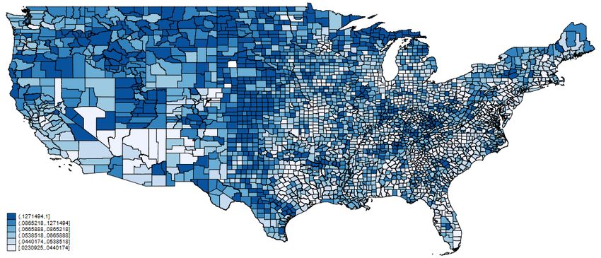
COMPETITION AND SELECTION IN CREDIT MARKETS

                                         Constantine Yannelis
                                         Anthony Lee Zhang

                                             August 2021

We are grateful to Scarlet Chen, Mark Egan, Piero Gottardi, Zhiguo He, Sasha Indarte, Ben Lester,
Jack Liebersohn, Willy Yu-Shiou Lin, Holger Mueller, Taylor Nadauld, Scott Nelson, Claudia Robles-Garcia,
and Amit Seru for helpful comments, as well as seminar participants at the Philadelphia Fed, NBER
Household Finance Summer Institute, Fourth Biennial Conference on Auto Lending, 2021 NASMES,
Barcelona GSE Summer Forum, Northwestern University Kellogg School of Management, UCLA
Andersen School of Business, Chicago Corporate and Household Lending Conference and the University
of Chicago Booth School of Business. Yannelis and Zhang gratefully acknowledge financial support
from the Booth School of Business at the University of Chicago. Livia Amato, Greg Tracey, Julian
Weber, and Xinkai Wu provided superb research assistance. TransUnion (the data provider) has the
right to review the research before dissemination to ensure it accurately describes TransUnion data,
does not disclose confidential information, and does not contain material it deems to be misleading
or false regarding TransUnion, TransUnion’s partners, affiliates or customer base, or the consumer
lending industry.

© 2021 by Constantine Yannelis and Anthony Lee Zhang. All rights reserved. Short sections of text,
not to exceed two paragraphs, may be quoted without explicit permission provided that full credit,
including © notice, is given to the source.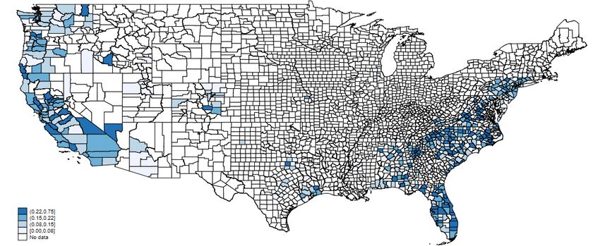
Competition and Selection in Credit Markets
Constantine Yannelis and Anthony Lee Zhang
August 2021
JEL No. D14,D4,G20,G21,G5,L62

                                          ABSTRACT

We present both theory and evidence that increased competition may decrease rather than
increase consumer welfare in subprime credit markets. We present a model of lending markets
with imperfect competition, adverse selection and costly lender screening. In more competitive
markets, lenders have lower market shares, and thus lower incentives to monitor borrowers. Thus,
when markets are competitive, all lenders face a riskier pool of borrowers, which can lead interest
rates to be higher, and consumer welfare to be lower. We provide evidence for the model’s
predictions in the auto loan market using administrative credit panel data.

Constantine Yannelis
Booth School of Business
University of Chicago
5807 S. Woodlawn Avenue
Chicago, IL 60637
and NBER
constantine.yannelis@chicagobooth.edu

Anthony Lee Zhang
University of Chicago
Booth School of Business
5807 S Woodlawn Ave
Chicago, Illi 60637
anthony.zhang@chicagobooth.edu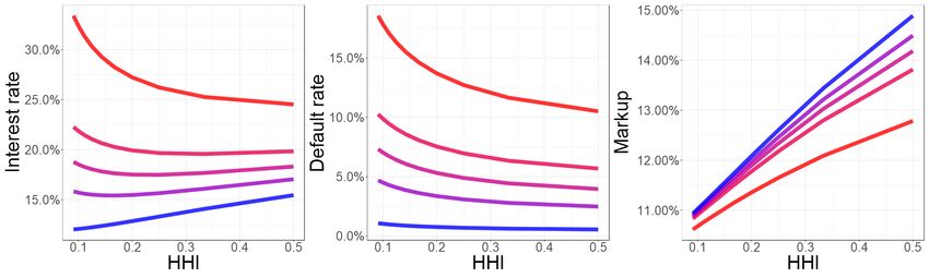
1        Introduction

How do the effects of market concentration interact with lender screening in credit markets?
The efficiency of lending markets can be hampered by information imperfections (Akerlof,
1970; Stiglitz and Weiss, 1981), but these harmful effects can be in part mitigated by imperfect
competition (Petersen and Rajan, 1995; Mahoney and Weyl, 2017). We propose and test a new
channel through which competition can have adverse effects on consumer credit markets.
        There is a theoretical reason to believe that credit market competition can harm consumers
in high-risk market segments. Lenders can invest in a fixed-cost screening technology, which
screens out consumers who are likely to default, allowing lenders to charge lower interest
rates to the remaining consumers.1 Lenders in concentrated markets have higher incentives
to invest in screening, since their fixed costs are divided among a larger customer base. As a
result, when market competition increases, lenders have lower incentives to invest in screening.
The population of borrowers becomes riskier, and interest rates can actually increase, leaving
consumers worse off.
        Our framework makes a simple and surprising empirical prediction. In low-risk market seg-
ments, loan rates should be positively associated with market concentration, as predicted by
classical theory. In high-risk segments, where screening is more important, loan rates should
actually be negatively associated with concentration measures. We test this prediction using
administrative credit panel data from TransUnion. We focus on auto lending, a rapidly grow-
ing consumer lending sector with $1.4 trillion in outstanding loan volume. Auto lending is
characterized by direct lending to consumers from banks and dealers, segmentation accord-
ing to consumers’ credit risk, and the absence of government subsidies and guarantees. All
of these features make the auto lending market ideal to explore the predictions of the theo-
retical model. We build a nationally representative dataset, at the county by year level, split
by VantageScore credit score bins. The model’s predictions hold in the data: concentration is
positively associated with interest rates for prime borrowers, and negatively associated with
rates for subprime borrowers.
    1
     Anecdotal evidence suggests that costly mechanisms which lenders use to screen borrowers are increasingly
common. For example, lenders can invest in better predictive analytics, for example using machine learning or
artificial intelligence. Lenders may also purchase data which can predict default. Some auto lenders also invest
in physical technology, such as GPS technology to track cars in the event of a repossession.

                                                       1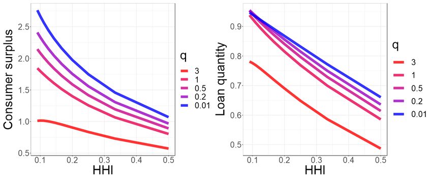
We analyze a simple model in which lenders invest in a technology to screen out consumers
likely to default, then compete by setting interest rates. In consumer lending settings, many
screening technologies are characterized by large upfront costs and low variable costs: lenders
often acquire alternative data on consumers, and hire employees to build default prediction
models and loan decision software. To model this, we assume that the screening technology
is fixed-cost: the lender’s cost depends on the desired default rate, but not on the number
of loans made. This implies that lenders who make more loans have larger incentives to in-
vest in screening, since the cost of screening is distributed over a larger consumer base. We
assume lenders are differentiated, so lenders are able to charge markups over their marginal
costs. In equilibrium, consumers’ interest rates are equal to the break-even interest rate, given
consumers’ default rates, plus a markup which depends on lenders’ market power.
   Competition has two opposing effects on interest rates. Competition tends to decrease
interest rates by lowering lenders’ market power: in more competitive markets, lenders set
smaller markups over their break-even rates. However, more competition implies that each
lender’s market share is lower, so lenders have lower incentives to invest in screening out
borrowers who are likely to default. Lenders thus face a riskier set of borrowers, and charge
higher rates as a result. When the market contains a large fraction of high-risk consumers,
the screening force can dominate, and equilibrium interest rates can actually increase, and
consumer welfare can decrease, as markets become more competitive.
   The main prediction of our model is that the relationship between concentration and inter-
est rates depends on the level of default risk in the population. Interest rates should increase
with market concentration in low-risk market segments, and interest rates should decrease
with concentration in high-risk market segments. The model also makes two auxiliary pre-
dictions. The first is that concentrated markets should always have lower default rates, since
lenders have higher incentives to screen. The second is that, in high-risk market segments,
higher concentration can simultaneously lead to lower quantities and lower prices, as lenders
with market power screen more intensively, but offer lower rates to borrowers that pass the
screening. This cannot occur in an environment without some form of screening or rationing:
demand curves slope downwards, so if lenders offered lower rates without screening, more
customers will want to borrow.

                                               2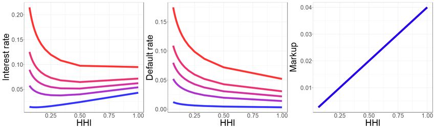
Consistent with our predictions, we find an opposite relationship between interest rates and
market concentration for low and high credit borrowers. For borrowers with high credit scores,
above 600, we find the classical relationship that interest rates are higher in more concentrated
markets. For borrowers with low credit scores, below 600, we find that interest rates are
actually lower in areas with more concentrated markets. The relationship is true in the cross
section, survives the inclusion of county and year fixed effects, and survives many alternative
strategies for measuring market concentration and interest rates. We also find direct evidence
that is suggestive that lenders engage in more screening in concentrated markets. In the cross-
section, lenders in more concentrated markets are more likely to purchase CreditVision, an
alternative data product sold by Transunion. Borrowers’ average credit scores are also higher in
more concentrated markets. We also find evidence for the other predictions of the model: in all
markets, delinquency rates are decreasing in market concentration, and in high-risk markets,
loan quantities are decreasing in market concentration, even though interest rates are also
decreasing.
   We further test our model’s predictions using bank failures and mergers as quasi-random
shocks to market competition. We link data on deposit shares from Federal Reserve call reports
to data on bank mergers and acquisitions from the National Information Center. Following
mergers, market concentration increases in counties with an acquired bank, and following
large bank failures, market concentration tends to decrease. In both cases, consistent with our
model’s predictions, we find that increases in concentration lead to higher interest rates for
high-credit-score consumers, but lower interest rates for low-credit-score consumers.
   We discuss and rule out several potential alternative channels. The interactive effects of
adverse selection and competition alone, as studied by Mahoney and Weyl (2017), cannot ex-
plain the results. With both competition and adverse selection, regardless of whether selection
is adverse or advantageous, market power increases prices. Theories of screening through con-
tract characteristics such as down payments also cannot explain our results (Veiga and Weyl
(2016)). Moral hazard, or higher interest rates having a causal effect on delinquency, also
cannot explain the results. In particular, moral hazard does not lead to higher competition
correlating with high interest rates for low credit score borrowers. Markups charged by auto
dealers cannot explain the asymmetry between low and high credit score individuals. Our re-

                                               3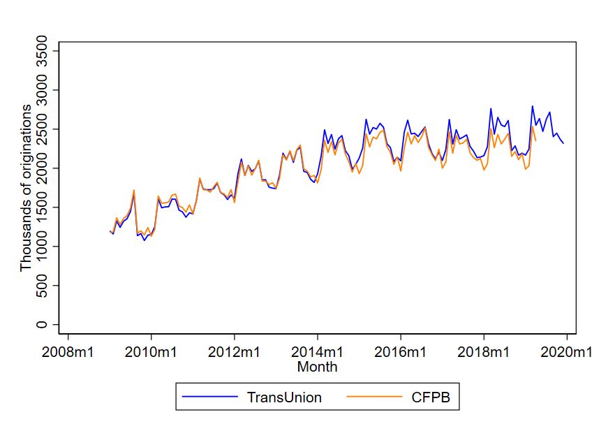
sults hold when we restrict the sample to pure auto lenders, or lenders (banks, credit unions,
and other entities) who make multiple kinds of loans, suggesting that our results are not driven
by heterogeneous funding costs for different kinds of lenders. Finally, since loan quantities are
decreasing in market concentration, the primary effect of competition appears to be through
screening, rather than improved collections technology, though this channel may also partially
contribute to the effects that we find.
   Our results imply that consumers may not always benefit from increased competition in
credit markets. In business lending, competition is known to have potentially adverse effects,
because it impairs the ability of banks to engage in relationship lending (Petersen and Rajan,
1995). This channel appears less relevant for consumer credit markets, since lender-borrower
relationships are likely less important for households relative to firms. Our results show that
competition can distort outcomes in consumer credit markets through a different channel.
   The channel in our paper is also distinct from that of, for example, Mian and Sufi (2009)
and Mahoney and Weyl (2017), who argue that credit market competition can lead to credit
over-provision. In these papers, increased competition lowers interest rates, and attracts bor-
rowers who are more likely to default. This may decrease social welfare, but always benefits
borrowers. In contrast, in our model, increased competition causes lenders to invest less in
screening, and instead to set higher interest rates for all consumers. This leads to inefficient
credit allocation, because lenders are less able to tell which consumers are creditworthy. In
our setting, increased competition can actually make consumers worse off.
   This paper joins a literature on the effects of competition in credit markets. This paper
presents a new model of competition in consumer credit markets, with the counterintuitive
result that in selection markets greater competition can actually harm consumers. Petersen and
Rajan (1995) study competition and relationship banking. Parlour and Rajan (2001) provide
a theoretical model of competition in loan contracts with multiple borrowers. Drechsler, Savov
and Schnabl (2017), Drechsler, Savov and Schnabl (2018) and Egan, Hortaçsu and Matvos
(2017) study deposit market concentration. Calomiris (1999) studies the efficiency of bank
mergers. Argyle, Nadauld and Palmer (2020b) study the real effects of search frictions in
auto lending and Buchak and Jørring (2021) study the effects of competition on lending and
discrimination in the mortgage market. There is also a large literature on the effects of bank

                                               4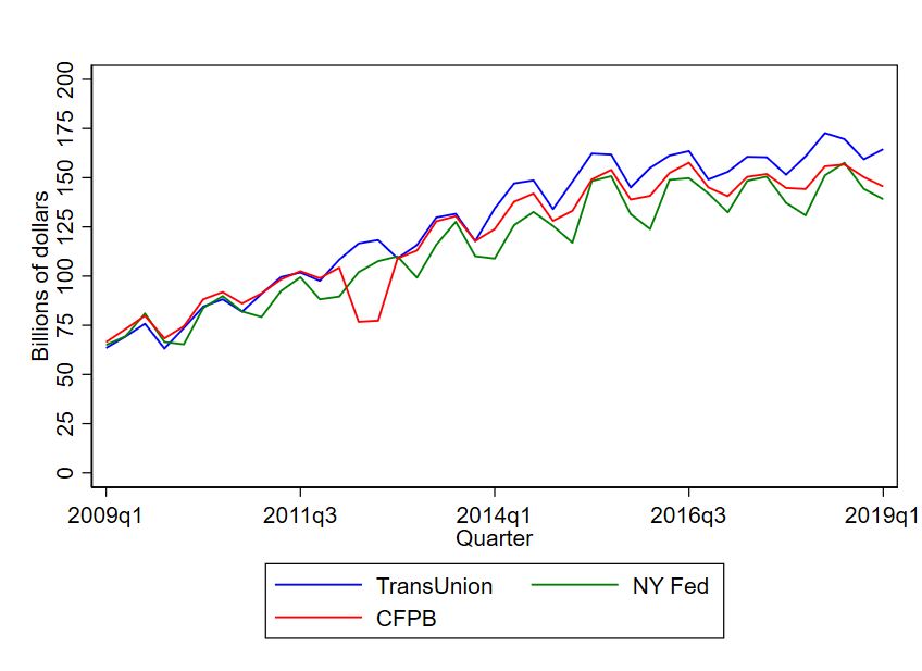
branching deregulation, for example Jayaratne and Strahan (1996), Economides, Hubbard and
Palia (1996), Krozner and Strahan (1999). Einav, Jenkins and Levin (2012) present a model of
subprime auto lending under imperfect competition with different risk types. Bank competition
is also known to affect local industry structure (Cetorelli and Strahan, 2006). Livshits et al.
(2016) study a model in which lenders have a fixed costs of contract design. The paper also
joins work on the relationship between monitoring and competition in finance. Giroud and
Mueller (2010) and Giroud and Mueller (2011) study the relationship between competition
and corporate governance. Consistent with interactive effects of monitoring and competition,
                                                                                                        2
they point to monitoring playing a more important role in less competitive industries.
       This paper also joins a body of work on the interaction of adverse selection and competition.
We show that, perhaps surprisingly, in some cases greater market concentration can benefit
consumers. Previous papers have rather focused on the fact that selection can mitigate the
harmful effects of market power. Mahoney and Weyl (2017) provide a model of imperfect
competition, and show that in the presence of adverse selection many of the harmful effects
of imperfect competition are mitigated. Lester, Shourideh, Venkateswaran and Zetlin-Jones
(2019) analyze competition and adverse selection in a search-theoretic model, finding that
increasing competition can decrease welfare. Crawford, Pavanini and Schivardi (2018) study
the interaction of competition and adverse selection in corporate credit markets. Vayanos and
Wang (2012) study the interaction of selection and competition in asset markets.
       This paper is also related to a theory literature on competition between banks, when banks
have imperfect information about borrowers’ default risk. An early paper in this literature is
Broecker (1990). He, Huang and Zhou (2020) studies competition in lending markets when
borrowers can decide whether to share data with lenders. Our signal structure is similar to
He, Huang and Zhou (2020): banks are able to screen out some bad types, and the remaining
population has a mix of bad and good types. Hauswald and Marquez (2006) analyzes a related
model, in which banks acquire information on borrowers distributed on a circle, and banks are
better at acquiring information on borrowers they are closer to. The main difference between
   2
     Most narrowly, this paper also joins a body of work on auto lending. For example, Adams, Einav and Levin
(2009) study liquidity constraints in subprime auto lending, Argyle, Nadauld and Palmer (2020a) study the
demand for maturity, Benmelech, Meisenzahl and Ramcharan (2017) study liquidity, Grunewald et al. (2020)
study dealers’ joint decisions of loan and car prices, and Einav, Jenkins and Levin (2013) study the introduction
of credit scoring.

                                                       5
our paper and this literature is that we assume information acquisition is a fixed cost, rather
than a variable cost. Variable-cost screening models are appropriate for modeling bank lending
to firms, where banks make relatively few loans, and the evaluation and underwriting process
is manual and relatively heterogeneous across firms. In contrast, consumer lending settings
generally involve screening technologies with large fixed costs and lower variable costs: lend-
ing decisions are often made using software, default prediction models, and more automated
processes.
The remainder of this paper is organized as follows. Section 2 presents our theoretical
model, and shows that, with monitoring and adverse selection, greater market concentration
can lead to a rise in prices. Section 3 presents data and institutional background. Section 4
presents empirical evidence consistent with our model. Section 5 discusses potential alterna-
tive channels. Section 6 concludes.
2 Model
We build a model in which differentiated lenders invest in a costly technology to screen po-
tential borrowers, and then set loan rates for lending to the borrowers. There are N lenders,
indexed by j.3 Lenders compete in a two-stage game. In the first stage, lenders simultaneously
choose how much to invest in screening out bad-type consumers. In the second stage, lenders
compete a la Bertrand, simultaneously posting interest rates at which they are willing to lend
to consumers.
Consumers. Each consumers wishes to borrow a unit of funds from lenders. There are
two types of consumers: there is a unit mass of type G consumers, and a measure q of type B
consumers. G consumers always pay back loans, and B consumers always default. We assume
for simplicity that type B consumers default without paying any interest, and that recovery
rates are always 0, so type B consumers cost lenders the principal of 1 and pay nothing. We
relax the assumption of zero recovery rates in Appendix A.4. In Appendix A.6, we assume there
is moral hazard for type G consumers: type G consumers default with some probability that
is increasing in the interest rate they are charged. In both cases, our results are qualitatively
3
In Appendix A.5, we show that N can be micro-founded as the equilibrium outcome from an entry game, in
which lenders sequentially decide whether to pay a fixed entry cost to enter the market.
6unchanged.
The willingness-to-pay of consumers for loans is independent of whether they are type B or
G. Consumers’ preferences over lenders are described by a Salop (1979) circle. The N lenders
are uniformly spaced around a unit circle, and consumers are arranged uniformly on the circle.
Consumers’ preferences for lenders are a function of distance: the utility of a consumer who
borrows from lender j, at loan rate r j , is:
µ − rj − θ x j (1)
where x j is the distance between the consumer and lender j on the circle. The constant µ
affects the total utility of the consumer for borrowing. We assume that µ is high enough that
consumers do not choose the outside option in equilibrium. We also assume that µ < 1, so that
type B consumers’ willingness-to-pay is never higher than the social cost, 1, of providing credit
to them, so it is socially inefficient to provide credit to type-B consumers. We use the Salop
circle because it is a simple model of imperfect competition, in which lenders set markups
which depend on the number of competitors present. In Appendix A.8, we show that our main
results also hold if borrowers’ preferences over lenders are instead described by a logit model.
Costly screening. We assume that lenders can invest in a fixed-cost screening technology to
imperfectly detect type-B consumers: by paying a fixed amount, lenders obtain a signal which
is informative about consumers’ types. We can think of auto lenders’ screening technologies
as, for example, acquiring alternative data, hiring employees to build default rate prediction
models and automated decision-making software. These technologies have large fixed-cost
components: building models or decision-making software has large upfront costs, but the
variable cost of scaling a model to more consumers is low.4
The assumption that screening has fixed costs is the main difference between our model and
much of the previous literature on bank lending, in which information acquisition is assumed to
be a variable cost, scaling linearly with the number of loans made (Broecker (1990), Hauswald
and Marquez (2003), Hauswald and Marquez (2006)). Information acquisition is likely to be
4
In the main text, we assume screening is entirely fixed-cost for expositional simplicity. However, our main
results hold screening has both fixed and variable cost components: as we show in Appendix A.4, any variable
cost of lending would simply increase interest rates uniformly.
7more variable-cost-intensive in firm lending settings, where banks make fewer loans, and tend
to manually review and underwrite each loan, in contrast to the more automated process in
consumer lending settings.
Formally, we assume that each lender j can pay a fixed cost to acquire an imperfect signal
of borrowers’ types. The signal has a “bad-news” structure: for type-G borrowers, the lender
always observes a good signal. For type-B borrowers, the signal is good with probability α j and
bad with probability 1 − α j , independently across borrowers. The cost of buying a signal with
strength α j is c̃ α j . We assume c̃ α j is strictly decreasing in α j : stronger signals (smaller α j )
are more expensive. Aggregating across borrowers, a measure q 1 − α j of type-B customers
will receive bad signals: lender j knows with certainty that these customers are type-B, and
will not lend to them.5 A measure qα j of type-B consumers receive good signals, and are
indistinguishable from the unit measure of type-G consumers. Since the cost c̃ α j does not
depend on the number of borrowers that the lender interacts with, signal purchasing is more
cost-effective if the lender has a larger share of the market.
In the main text, we assume that type B consumers are ordered in terms of how easy they
are to screen. Thus, if all firms attain a signal with strength α, they screen out exactly the same
measure qα of consumers. This implies that, in any symmetric equilibrium where firms choose
the same value of α, firms’ signals about consumers are perfectly correlated: a consumer who
is detected as a type-B by one firm is detected by all other firms, and any type-B consumers
who are not detected are treated identically by all firms.6
If the population fraction of type-B consumers is q, and lender j chooses signal strength α j ,
the default rate among borrowers with good signals is:
αjq
δj = (2)
1 + αjq
5
Since type-B consumers always default, and never pay interest or principal, there is no rate at which it is
profitable to lend to them.
6
If firms’ signals are not perfectly independent across customers, firms would be able to infer additional infor-
mation about customers’ types from whether other firms are willing to lend to customers, so the inferred default
rates among marginal consumers are different from default rates among average consumers. This complicates
the model without adding significant insight, so we assume this away in the main text. However, we partially
relax this assumption in appendix A.7, and show it does not affect our main results.
8Inverting, in order to attain default rate δ j , lenders must choose:
δj
αj =
q 1 − δj
We can thus think of lenders as choosing a desired default rate δ j . The cost of attaining default
rate δ j , when the population measure of bad types is q, is:
δj
cq δ j = c̃ (3)
q 1 − δj
Note that, since c̃ is decreasing, the function cq δ j is increasing in q, fixing δ j : when there
are more bad types in the population, it is more costly to attain any given default rate, because
the lender must acquire a stronger signal (a lower value of α j ) to do so.
2.1 Equilibrium
We restrict to symmetric equilibria of the model, in which lenders make optimal screening
and price-setting decisions. We solve the model backwards, solving for optimal price-setting
decisions given default rates, and then solving for optimal screening decisions. First, note that
in any symmetric equilibrium, lenders set identical interest rates, and each lender has market
share:
1
sj =
N
Price setting. After screening is complete, lenders simultaneously set interest rates for
customers who are not screened out as bad types. In the main text, we assume lenders can
borrow at zero interest rates; we relax this in Appendix A.4. Lender j thus chooses r j to
maximize:
1
Π= sj rj 1 − δj − δj (4)
1 − δj
1
where s j is j’s market share, and the total measure of customers that pass j’s screening is 1−δ j
.
Intuitively, (4) says that, with probability 1 − δ j , the customer borrows a unit of funds, and
pays back 1 + r j , so the lender’s profit is r j . With probability δ j , the customer defaults, and the
9lender loses the principal of 1. Lenders’ profits can be rearranged to:
δj
Π = sj rj − (5)
1 − δj
In Appendix A.1, we show that lender j’s optimal interest rate r j , in symmetric equilibrium,
satisfies:
δj θ
rj − = (6)
1 − δj N
δ δj
The intuition for (6) is that r j − 1−δj j , the markup of r j over the break-even interest rate, 1−δ j , is
higher when θ is higher, so consumers are more distance-sensitive and thus less price-sensitive,
and when N is lower, so markets are more concentrated.
Optimal screening. Lender j chooses a desired default rate δ j to maximize total lending
profits, minus screening costs cq δ j . That is, lender j solves:
δj
max max s j r j rj − − cq δ j (7)
δj rj 1 − δj
In Appendix A.2, we characterize first- and second-order conditions for lenders’ optimal infor-
mation acquisition decisions. The first-order condition is:
sj
2 = −cq δ j
0
(8)
1 − δj
Intuitively, the left-hand side of (8) is the marginal benefit of decreasing the default rate δ j by
a small amount, which is higher when j’s market share, s j , is higher.7 The right-hand side is
the marginal cost of decreasing δ j , which depends on the fraction of type-B consumers in the
population.
Combining (6) and (8), the following proposition states conditions on r, s, δ which charac-
terize a symmetric equilibrium.
Proposition 1. Necessary conditions for a symmetric equilibrium are that all lenders’ market
7
While we focus on market shares, the average fixed cost decreases with market size. This is explored in the
appendix, and we find empirical results consistent with stronger asymmetric effects in larger markets.
10shares s, default rates δ, and interest rates r as are follows. Market shares of each lender are:
1
s= (9)
N
Lenders must set prices optimally:
δ θ
r− = (10)
1−δ N
All lenders must make optimal screening decisions:
1
2
= −cq0 (δ) (11)
N (1 − δ)
2
cq00 (δ) (1 − δ)4 + (1 − δ) > θ (12)
N
Total loan quantity is:
1
1−δ
In any equilibrium, total consumer welfare of type G consumers is:
θ
µ−r − (13)
4N
Note that expression (13) for consumer surplus only accounts for type G consumers. This
allows us to illustrate how non-defaulting consumers, who always have a willingness-to-pay
which is higher than the cost of providing credit to them, are affected by the two forces of
market power, and imperfect screening by lenders, which causes them to pool with type B
consumers.8
We proceed to solve the model numerically. For our simulations, we assume costs take the
form:
k
c̃ (α) =
α
8
Since we have assumed that the social cost of providing credit to type B consumers is higher than their
value for loans, it is never socially efficient to lend to type B consumers. Thus, screening also increases total
social efficiency of credit allocation, by decreasing lending to type B consumers. We focus attention on the two-
type case to capture the main qualitative insights of the setting. In a richer model with more than two types of
consumers, screening could potentially have more complex distributional implications: an imperfect screening
technology could reduce credit to some consumers who should receive credit in the first-best allocation.
11Plugging into (3), this implies that:
kq 1 − δ j kq
cq δ j = = − kq (14)
δj δj
Expression (14) shows that screening costs are increasing in the parameter k, and the measure
of type-B consumers, q. When q is large, screening costs are high, and it is more costly on the
margin to decrease the default rate δ by any given amount. When q is 0, there are no bad
types in the population, so it is costless for the firm to achieve a default rate of 0.
Figure 1 shows equilibrium outcomes, as we vary the number of lenders, for different levels
of q. Throughout, we fix k = 0.001, as this generates realistic numbers for interest rates. The
x-axis of each plot is the Herfindahl-Hirschman index:
X
HHI ≡ s2j
j
1
In our model, this is simply N. The top-left panel shows the interest rate, r. When q is low, so
the consumer population is low-risk, the relationship between r and competition is consistent
with classical theory: interest rates are higher when H H I is higher and markets are more
concentrated. However, when q is high, so the population is risky, we obtain the opposite result:
interest rates are actually lower when when H H I is higher and markets are more concentrated.
To illustrate the forces driving this results, the top-middle plot shows the default rate δ,
and the top-right plot shows the equilibrium markup charged by lenders over the break-even
δ
price, r − 1−δ . The top-middle plot shows that the default rate δ is always decreasing in H H I,
regardless of q. Intuitively, when H H I is higher, firms have larger market shares, and thus
higher incentives to invest in screening, lowering equilibrium default rates. The slope of the
H H I-δ curve depends on q, the level of risk in the population.
The top right plot shows the markup that firms charge over the break-even price in equi-
δ
librium, r − 1−δ . Markups are always higher in more concentrated markets, since firms have
more market power. However, unlike default rates, the effect of concentration on markups is
insensitive to the average riskiness of the borrower population.
The net effect of concentration on interest rates combines the effects of concentration on
12default rates and on markups. When q is low and the population is low-risk, the markup effect
tends to dominate, so interest rates are increasing in concentration. When q is high and the
population is high-risk, the screening effect tends to dominate, and interest rates are decreasing
in concentration. The effect of concentration on default rates can be strong enough that the
welfare of good-type consumers is actually higher in more concentrated markets: the bottom
left panel shows that, when q is large, consumer surplus increases as H H I increases.
The bottom right panel of Figure 1 shows total loan quantities as a function of concen-
tration. In our model, loan quantity tends to decrease when concentration is higher. This is
true even when q is high, and concentration is negatively correlated with interest rates. This
is because lenders screen more in more concentrated markets, removing bad types from the
population, and thus decreasing equilibrium loan quantities, even though interest rates are
lower.
Based on Figure 1, we can derive three testable predictions to bring to the data.
Prediction 1. When the level of default risk in the consumer population is low, higher concentra-
tion tends to increase interest rates. When the population default risk is high, concentration tends
to decrease interest rates.
This follows from the top left panel of Figure 1. The next prediction concerns default rates,
from the top-middle panel.
Prediction 2. Higher concentration always leads to lower default rates.
Finally, the bottom-right panel of Figure 1 makes a prediction about loan quantities.
Prediction 3. When the population default risk is high, higher concentration can simultaneously
lead to lower interest rates and lower loan quantities.
The intuition behind Prediction 3 is that, in high-risk markets, lenders screen more, limiting
the set of consumers that receive loans, and offer lower interest rates to these consumers. This
cannot occur in an environment without screening: market demand curves slope downwards,
so lower prices will always lead to higher quantities, if all customers are allowed to borrow at
the market price.9
9
We note that, in the baseline model, quantities are always decreasing in concentration, because there is no
133 Data and Institutional Background
3.1 Institutional Background
While the model presented in section 2 can broadly apply in consumer credit markets, we focus
our empirical analysis on auto loans for three reasons. First, the institutional details pertaining
to auto lending are relatively simple and direct relative to other large consumer loan markets,
like the mortgage and student loan markets. Second, the auto loan market is largely segmented
along borrower riskiness. Borrowers with different credit scores and risk tend to purchase
different vehicles and utilize different lenders. Finally, unlike mortgage and student loans,
auto lending is typically not guaranteed, and so losses are directly incurred to the lender– an
important feature of our model. Relatedly, securitization can also change lenders’ incentives
to screen borrowers (Keys, Mukherjee, Seru and Vig, 2008), and one attractive feature of the
market is that auto loans are also less likely to be securitized relative to mortgage loans.
Auto loans are the third largest source of household debt in the United States, following
mortgage and student loans. The Federal Reserve Bank of New York reports approximately
$1.4 trillion in outstanding auto loan debt in 2020.10 The vast majority of auto purchases in
the US are financed. Over 95% of American households own cars and the National Association
of Auto Dealers estimates that in 2019, 85% of new vehicles and 55% of used vehicles were
purchased using auto loans. According to Experian, in 2020 31.2% of auto loans were made
by captive subsidiaries, 30.2% were made by banks, 18.7% were made by credit unions, 12.4%
by finance companies and the remaining 7.6% by dealers themselves.11
There are two types of auto lending, direct and indirect. Direct lending implies that con-
sumers take a loan directly from a financial institution, and use that to purchase a vehicle.
The consumer will submit information to a lender, and the lender will decide whether to ap-
prove the loan. Under indirect lending, the consumer applies for a loan through the dealer
extensive margin: customers never choose not to borrow. Thus, total loan quantity depends only on lenders’
screening decisions: when markets are more concentrated, lenders screen more intensively, so total loan quantity
decreases. In a richer model, such as that of Appendix A.8, prices would also affect customers’ choices on the
extensive margin, so higher concentration can conceivably lead to higher quantities, if lenders can lower prices
sufficiently to attract many more type-G customers into the market.
10
Levitin (2020) provides a detailed description of the auto loan market.
11
In the appendix, we show that our results hold if we restrict to banks and other lenders that do not exclusively
offer auto loans.
14and dealers obtain financing through third party lenders. Dealers typically have relationships
with several lenders, and after providing lenders with borrower information the dealers solicit
offers for the minimum interest rate that a lender will provide.
Importantly for linking to our model, auto loans typically remain on lenders’ books. Hence
lenders incurs costs if borrowers default. In 2020, only 14% of auto loans were securitized
according to SPG Global.12 A slightly higher fraction of subprime loans are securitized, but the
vast majority – three quarters – of subprime auto loans are not securitized.
3.1.1 Monitoring
Beyond the most basic form of screening, accepting or rejecting clients based on credit scores,
there are a number of ways in which auto lenders monitor borrowers. These methods typically
incur costs to lenders. For example, some auto lenders install GPS tracking to be better able
to repossess vehicles in the case of default. Lenders can also invest in predictive analytics,
sometimes using machine learning and artificial intelligence, to identify which borrowers are
less likely to default, even within subprime categories. Modeling prepayment risk can also
allow lenders to go beyond traditional credit scoring. Some lenders also verify a car’s con-
dition before lending to risky borrowers, since lemons are useless as collateral. All of these
actions would lead to better screening and monitoring of borrowers, but would incur costs
for the lender either through building better predictive analytics, paying to inspect vehicles or
installing additional features to track vehicles.
In our analysis, we will use county-year HHI as a measure of market competition. This
implicitly assumes it is a lender’s local market share which matters for screening decisions,
which would be reasonable if lenders’ screening decisions are local in nature. There are a
number of reasons why this might be the case. First, most auto loans are made through lenders’
relationships with dealers. If lenders need to invest in dealer-specific information acquisition,
for example to determine dealerships with higher default rates, these investments would be
location-specific in nature. Second, some information used to estimate default risks is very
local in nature. For example, borrowers living in certain neighborhoods may have different
12
Similarly, Klee and Shin (2020), using data from SIFMA, state that the quantity of outstanding auto ABS was
around $225 billion in 2018, which is around 18% of the total outstanding volume of auto loans.
15default risks than others; detecting these relationships and using them to price loans may
require location-specific data acquisition and analysis.13
3.2 Data
3.2.1 Booth TransUnion Consumer Credit Panel
Our main data source is the Booth TransUnion Consumer Credit Panel. The data is an anonymized
10% sample of all TransUnion credit records from 2009 to 2020. Individuals who were in the
initial sample in 2000 have their data continually updated, and each year 10% of new first
time individuals in the credit panel are added. A small fraction of individuals also leave the
panel each year, for example due to death or emigration.14 We define markets at the county
level, and our main analysis dataset consists of new loans at the county by credit score by year
level. We drop observations with fewer than ten loan contracts annually.
We can observe basic information about a loan, including the original balance, the current
balance, scheduled payments, and maturity of the loan. We can also observe other borrower-
level information, including VantageScore and geographical variables. Interest rates are not
directly observed, and thus we back these out using scheduled payments. We take the first
observation for each loan and use the amortization formula to calculate interest rates A =
P×i
1−(1+i)−n , where A is the monthly payment due, P is the principal amount on the loan, n is the
maturity in months, and i is the interest rate, we solve for i using a root-solving algorithm,
after removing missing observations for each requisite variable.15 The identities of the lender
that originated the loan, as well as the loan customer, are anonymized by the data provider.
Total loan volumes in our data are also comparable to measures from other datasets: we
plot the time series of the total number and dollar volume of car loans from different datasets
in Appendix Figure A.4. Appendix Figure A.5 shows the distribution of consumers by credit
13
Address history and property values appear to be important components of some alternative credit data
products. See, for example, LexisNexis RiskView.
14
Keys, Mahoney and Yang (2020) provide more details about the Booth TransUnion Consumer Credit Panel and
Herkenhoff, Phillips and Cohen-Cole (2019) and Braxton, Herkenhoff and Phillips (2020) more generally discuss
TransUnion data. All tables and figures that list TransUnion as a source have statistics calculated (or derived)
based on credit data provided by TransUnion, a global information solutions company, through a relationship
with the Kilts Center for Marketing at the University of Chicago Booth School of Business.
15
We drop a small number of observations where predicted interest rates are either negative or implausibly
large. We further winsorize rates at the .2% level.
16score in our data. The average interest rate in our sample is 9.3%, which compares to averages
rates of 5.9% for new vehicles, and 9.5% for used vehicles, from the National Association of
Auto Dealers. Interest rates are much higher for groups with lower credit scores. In the lowest
credit score groups in our sample (below 600), the average interest rate is 15.07%. This is
approximately four times the average interest rate in the highest credit score group (above
800), which is 3.67%.16 These patterns likely reflect greater charge-off probabilities for low
credit-score borrowers. In the lowest credit score group, the average 90-day delinquency rate
is 34.26%, while it is 1.06% for the highest credit score group.
Our primary measure of market competitiveness is the Herfindahl–Hirschman Index, or
HHI. We construct HHI using the volume of auto loans, that is
N
X
H H Ic t = scl2 t (15)
l=1
where scl t is a lender l’s dollar share of auto lending in a county c in year t within a credit score
range. An HHI of zero means the market is perfectly competitive, while an HHI of one indicates
monopoly. The average HHI in our sample is .05, suggesting that the auto lending market is on
average quite competitive. Appendix Figure A.6 shows the geographic distribution of HHI.17
TU also provides novel data on Creditvision, a proprietary product which lenders can
purchase. Creditvision contains additional information on consumer behavior and histories.
Lenders who access Creditvision have additional tools that can be used to screen borrowers,
including predictive modeling, purpose-built scores, propensity models, attributes, algorithms,
and estimators. The Creditvision data is available at the state level, from 2016 to 2019. We
observe the total number of lenders active in a state, and the total number of lenders that
purchased the product from TU.
16
These are quite similar to rates published by Experian in 2020. The average rate for Deep Subprime borrowers
with credit scores below 580 is 14.39% for new cars, and 20.45% for used cars. For Subprime borrowers with
credit scores between 580 and 620 the corresponding rates are 11.92% and 17.74% respectively. For Super Prime
borrowers with scores above 720, the average rate for a new car loan is 3.65% and the average rate for a used
car loan is 4.29%.
17
When we restrict to bank lenders, the HHI is .12. This is comparable to estimates in the literature. For
example, Kahn, Pennacchi and Sopranzetti (2005) estimate an average MSA-level HHI of of .14 for commercial
banks’ personal and auto loan market shares from 1989-1997, and Drechsler, Savov and Schnabl (2017) estimate
an average county-level HHI of .22 for banks’ deposit market shares from 1994-2014.
173.2.2 Bank Merger Data
We complement our main analysis with data on bank mergers. We obtain deposit shares from
Federal Reserve Call reports. The bank mergers data is collected from the transformations file
from the National Information Center (NIC). We assume that a county is affected by a merger
if an acquired bank has positive deposit market share in the county. In cases with more than
one merger, we use the first merger event. Between 2009 and 2019 there are a total of 1,442
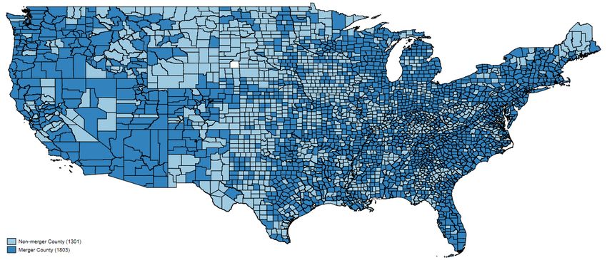
mergers, covering 1,812 distinct counties.
Appendix Figure A.12 shows the geographical distribution of mergers. More than half of
the counties in our sample are affected by a merger at some point in our sample period, and
the affected counties seem to be fairly uniformly distributed across the US. Appendix Figure
A.13 shows a binscatter of bank deposit market HHI, measured using the summary of deposits
data, on the x-axis, with auto lending HHI, measured in the TransUnion data, on the y-axis.
Auto lending HHI and bank deposit HHI are very strongly correlated, suggesting a tight link
between the two.
4 Empirical Evidence
4.1 Interest Rates, Competition and Credit Scores
Prediction 1 of the model states that, when the population is low-risk, and screening costs
are low, we see the classical relationship that competition tends to be associated with lower
interest rates. When the population is high-risk, and screening costs are high, we see the
opposite relationship that competition should be associated with higher interest rates. This
prediction is borne out by the data.
Figure 2 presents our main result. The figure panels show median interest rates in a county
for given credit score ranges, broken down in twenty equal-sized bins of HHI, our measure
of the competitiveness of a market. The left panel shows the relationship for borrowers with
VantageScore scores below 600, while the right panel shows the relationship for borrowers with
VantageScore scores above 600. The two panels display strikingly different patterns, consistent
with our model presented in Section 2. The left panel, which covers high-risk borrowers,
18shows a strong, linear and negative relationship: in contrast with standard economic theory,
interest rates are actually decreasing in market concentration. The right panel, which shows
the relationship for low-risk borrowers, shows precisely the opposite relationship. Consistent
with a standard framework, we see that interest rates are increasing in market concentration.
The magnitudes of both relationships are fairly large: an increase in HHI from 0.05 to 0.15 is
associated with approximately a 1% decrease in interest rates for high-risk borrowers, and a
1% increase in interest rates for low-risk borrowers.
Figure 3 shows the same relationship, broken down into finer credit score categories. We
split the sample into six credit score bins. We see the strongest negative relationship between
interest rates and concentration for deep subprime borrowers, with credit scores lower than
550. We see a flatter relationship for credit scores between 550 and 600, and for credit scores
above 600 we generally see the classical relationship that interest rates are rising in concen-
tration.
Table 2 presents similar information to the figures by presenting regression coefficients.
More specifically, the table shows point estimates β and standard errors from specifications
similar to
ln(rc t ) = αc + α t + β ln(H H I c t ) + "c t (16)
where rc t is the average interest rate for auto loans in a county, and H H I c t is the Herfindahl–
Hirschman Index measuring market concentration. We cluster standard errors at the county
level. The main coefficient of interest β captures the effect of market concentration on interest
rates. We run estimates of specification (16) separately by different credit score buckets.
We additionally include county fixed effects αc , which absorb time invariant county spe-
cific factors, such as geographic areas having riskier drivers, and α t time fixed effects absorbing
economy wide temporal shocks. The inclusion of time trends is particularly important, as they
allow us to rule out that the observed patterns in Figure 2 are driven by temporal trends in
both interest rates, credit scores and HHI. For example, in the absence of time fixed effects, it is
possible that the differing relationships between the slopes of interest rates and market concen-
tration are simply driven by a decline in the fraction of low-credit score borrowers coinciding
with movements in interest rates and market concentration.
The top panel of Table 2 splits the sample between credit scores above and below 600, and
19gradually adds in fixed effects. The first column of each triplet has no fixed effects, the second
column adds in year fixed effects, while the final columns adds in both year and county fixed
effects. In all three cases, we see a similar pattern and magnitudes. For borrowers with lower
credit scores, we see that a 1 percent increase in market concentration, as measured by HHI,
is associated with a .07 to .08 percent decrease in interest rates. The relationship is statistically
significant at the 1% level in all specifications. For high-credit score borrowers, we observe the
opposite relationship. A 1 percent increase in market concentration, as measured by HHI, is
associated with a .19 to .30 percent increase in interest rates. The relationship is slightly weaker
for high-credit score borrowers, significant at the 5% or 10% level in each specification.
The bottom panel of Table 2 splits the sample into finer credit score bins, including county
and year fixed effects. We find a strong and highly significant negative relationship between
interest rates and concentration for borrowers with credit-scores below 600, and a positive
and significant or marginally significant relationship for borrowers with credit-scores above
600. The relationship is generally increasing as credit scores improve, consistent with the
predictions of the model.
Table 3 presents an alternative specification, interacting HHI with credit score groups (above
or below 600.) Specifically, the table shows variants of the coefficient γ and φ from the equa-
tion
l n(rcst ) = αcs + α t + γln(H H I c t ) × 1[C r edi tScor e Low ] + φln(H H I c t ) + ςcst (17)
1[C r ed i tScor e Low ] is an indicator of borrowers being in the low credit score group and αcs
are county by score group fixed effects. Standard errors are clustered at the county level. The
coefficient φ captures the effect of market concentration on interest rates for high credit score
borrowers, while γ + φ captures the effect for low credit score borrowers.
Column (1) of Table 3 presents the baseline result. Consistent with the estimates in Ta-
ble 2, we see a positive effect of market concentration on interest rates for high credit score
borrowers, and a negative effect for low credit score borrowers. Effects are highly statistically
significant, at the 1 percent level. This result holds without weighting counties (column 2),
using only large counties (column 3), using all counties (column 4), and winsorizing interest
rates at the 1% level instead of the .2% level (column 5). Column 6 shows the results from
computing HHIs using loan number as a measure of market share, instead of loan values. The
20effect of HHI in the high-credit-score group becomes insignificant, but the effect for low-credit-
score consumers remains negative and significant. Column 7 uses the number of lenders active
in a county as a measure of competition, instead of HHIs: the effect is insignificant for high-
credit-score consumers, but for low-credit-score consumers, counties with more lenders tend
to have higher interest rates. Appendix Figures A.7 and A.8 repeat the binscatters of Figure 3
with these different specifications; the stylized facts from the baseline specification hold in all
cases.
For large lenders, screening decisions may be made at more aggregated levels than counties:
for example, lenders may use the same analytics and decision software across branches in
multiple regions. Thus, larger lenders’ screening decisions should be less sensitive to local
market HHIs. On the other hand, if lenders set loan markups at the level of local markets, the
competition channel should affect large and small lenders similarly. This implies that interest
rates should be more positively correlated with HHIs for larger lenders, since the competition
channel plays a larger role than the screening channel.
To test this hypothesis, Appendix Table A.3 interacts HHI with the total volume of outstand-
ing loans and the number of counties in which a lender is active. As predicted, we find that
the interaction effect between HHI and both lender size measures is positive, for both prime
and subprime groups. In words, local concentration is more positively associated with inter-
est rates for larger lenders. Extrapolated out of sample, the estimates in Appendix Table A.3
suggest that under a monopoly, interest rates will be 9.1 percentage points lower for subprime
borrowers for a lender operating in a single county, but only 5.9 percentage points low for a
lender operating in all counties in the United States. Notice, however, that the relationship
between local HHIs and interest rates is negative even for large lenders; this suggests that,
even for large lenders, local factors may play some role in screening.18
4.2 Direct Evidence of Screening
We next provide suggestive evidence that lenders engage in more screening in more concen-
trated markets. Figure 4 presents more direct evidence that lenders engage in more screening
18
One example of this could be investing in relationships with dealers, or otherwise acquiring local information.
For example, Bank of America operates a large dealer network dealer network.
21in more concentrated markets. The figure shows that in the cross section, lenders in more
concentrated markets purchase more information on borrowers, and borrowers have higher
credit scores.
The top panels show the fraction of lenders purchasing Creditvision, by ventiles of HHI.
Creditvision is a proprietary product from TU, which contains additional information on con-
sumer behavior and histories. Creditvision includes predictive modeling, purpose-built scores,
propensity models, attributes, algorithms, and estimators. The data is available at the state
level, from 2016 to 2019. We construct auto loan HHI at the state level. The left panel shows
the relationship between Creditvision purchasing and HHI based on the volume of loans, while
the right panel shows the same relationship using a measure of HHI based on the number of
loans.
Both panels show a similar relationship consistent with our model: in more concentrated
markets, lenders are more likely to purchase additional information from TU. Regressing the
fraction of lenders purchasing Creditvision on the volume-based measure of HHI yields an
OLS coefficient of 0.965 and a standard error of 0.437, clustered at the state level. A similar
regression using the number of loans based measure of HHI yields a coefficient of 0.881 with
a standard error of 0.335.
The bottom panels show average credit scores in a county, by ventiles of HHI. Again the
left panel shows the relationship between credit scores and volume based HHI, while the right
panel shows the relationship using a measure of HHI based on the number of loans. Consistent
with more screening in concentrated markets, we see higher credit scores in more concentrated
markets. Regressing the fraction of lenders purchasing Creditvision on the volume-based mea-
sure of HHI yields an OLS coefficient of 22.97 with a standard error of 4.354, clustered at the
county level. A similar regression using the number of loans based measure of HHI yields a
coefficient of 22.80 and a standard error of 1.443.
4.3 Loan Delinquencies
We next turn to the relationship between market concentration and loan delinquency rates.
Prediction 2 of the model states that lower competition always leads to lower default rates.
This prediction is again consistent with the data.
22We estimate variations of equation (16), in which the outcome is the fraction of loans that
ever become delinquent for more than ninety days. Table 4 presents estimates of the relation-
ship between delinquency and market concentration. Consistent with the predictions of the
model and concentration leading to more monitoring, we see a negative relationship between
delinquency and concentration. The effect sizes change significantly when county fixed effects
are included, suggesting that it is important to control for regional heterogeneity. We find a
significant negative relationship between delinquency rates and HHI for borrowers with low
credit scores, and a statistically insignificant relationship for high credit score borrowers.
The bottom panel of Table 4 splits the sample in finer credit score bins, again including
county and year fixed effects. Consistent with the theory, in all estimates the observed rela-
tionship is negative. The results suggest that a 1 percent increase in market concentration is
associated with a .3 to .12 percent reduction in delinquency rates. The estimates are statisti-
cally significant at the 5% or higher level, except for the most creditworthy borrowers. This
lack of statistical significance in the top bin may simply be due to a lack of variation in the
dependent variable, as very few borrowers with high credit scores become delinquent on their
loans.
4.4 Loan quantities
Next, we test Prediction 3, regarding the relationship between concentration, interest rates,
and loan quantities in low credit-score buckets. In Table 5, we estimate panel regressions, in
which we regress the log of loan quantity on the log of HHI. We use only panel regressions, since
cross-sectional variation in loan quantities likely is driven largely by the size and demographic
composition of counties.
For all credit score buckets, the panel coefficients are negative and statistically significant,
implying that increases in county HHIs are associated with decreases in the number of loans
made. Quantitatively, a 1% increase in HHI is associated with a 2.7% to 5.2% decrease in loans
made. The coefficients tend to be larger for lower credit score groups.
For consumers with credit scores above 600, we found that higher concentration is asso-
ciated with higher interest rates. These patterns are consistent with classical intuitions about
market power: in concentrated markets, firms set higher prices, reducing equilibrium quanti-
23You can also read