The AquiFR hydrometeorological modelling platform as a tool for improving groundwater resource monitoring over France: evaluation over a 60-year ...
←
→
Page content transcription
If your browser does not render page correctly, please read the page content below
Hydrol. Earth Syst. Sci., 24, 633–654, 2020
https://doi.org/10.5194/hess-24-633-2020
© Author(s) 2020. This work is distributed under
the Creative Commons Attribution 4.0 License.

The AquiFR hydrometeorological modelling platform as
a tool for improving groundwater resource monitoring
over France: evaluation over a 60-year period
Jean-Pierre Vergnes1 , Nicolas Roux2 , Florence Habets3,4 , Philippe Ackerer5 , Nadia Amraoui1 , François Besson6 ,
Yvan Caballero1 , Quentin Courtois7 , Jean-Raynald de Dreuzy7 , Pierre Etchevers6 , Nicolas Gallois8 ,
Delphine J. Leroux2 , Laurent Longuevergne7 , Patrick Le Moigne2 , Thierry Morel9 , Simon Munier2 ,
Fabienne Regimbeau6 , Dominique Thiéry1 , and Pascal Viennot8
1 Water, Environment, Processes and Analyses Division, BRGM – The French Geological Survey,
45060 Orléans CEDEX 2, France
2 National Centre for Meteorological Research (CNRM) UMR 3589, Météo-France/CNRS,

University of Toulouse, 31100 Toulouse, France
3 CNRS UMR 7619 Milieux Environnementaux, Transferts et Interactions dans les hydrosystèmes et les Sols (METIS),

Sorbonne University, 75252 Paris CEDEX 5, France
4 Geology Laboratory of Ecole Normale Supérieure, Pierre Simon Laplace Research University,

CNRS UMR 8538, 75005 Paris, France
5 Laboratory of HYdrology and GEochemistry of Strasbourg (LHYGES), UMR 7517 CNRS,

EOST/University of Strasbourg, 67084 Strasbourg, France
6 Direction du Climat et des Services Climatiques (DCSC), Météo France, 31057 Toulouse CEDEX 1, France
7 Géosciences Rennes, UMR 6118, CNRS, University of Rennes I, 35042 Rennes CEDEX, France
8 Geosciences Research Department, MINES ParisTech, 77305 Fontainebleau, France
9 Centre Européen de Recherche et de Formation Avancée en Calcul Scientifique (CERFACS),

31057 Toulouse CEDEX 01, France

Correspondence: Jean-Pierre Vergnes (jp.vergnes@brgm.fr)

Received: 12 April 2019 – Discussion started: 22 May 2019
Revised: 17 January 2020 – Accepted: 20 January 2020 – Published: 13 February 2020

Abstract. The new AquiFR hydrometeorological modelling         proach using the EROS (Ensemble de Rivières Organisés en
platform was developed to provide short-to-long-term fore-     Sous-bassins; set of rivers organized in sub-basins) software
casts for groundwater resource management in France. This      programme. AquiFR computes the groundwater level, the
study aims to describe and assess this new tool over a long    groundwater–surface-water exchanges and the river flows. A
period of 60 years. This platform gathers in a single numer-   simulation covering a 60-year period from 1958 to 2018 is
ical tool several hydrogeological models covering much of      achieved in order to evaluate the performance of this plat-
the French metropolitan area. A total of 11 aquifer systems    form. The 8 km resolution SAFRAN (Système d’Analyse
are simulated through spatially distributed models using ei-   Fournissant des Renseignements Adaptés à la Nivologie)
ther the MARTHE (Modélisation d’Aquifères avec un mail-        meteorological analysis provides the atmospheric variables
lage Rectangulaire, Transport et HydrodynamiquE; Mod-          needed by the SURFEX (SURFace EXternalisée) land sur-
elling Aquifers with Rectangular cells, Transport and Hy-      face model in order to compute surface runoff and ground-
drodynamics) groundwater modelling software programme          water recharge used by the hydrogeological models. The as-
or the EauDyssée hydrogeological platform. A total of 23       sessment is based on more than 600 piezometers and more
karstic systems are simulated by a lumped reservoir ap-        than 300 gauging stations corresponding to simulated rivers

Published by Copernicus Publications on behalf of the European Geosciences Union.
634                                               J.-P. Vergnes et al.: The AquiFR hydrometeorological modelling platform

and outlets of karstic systems. For the simulated piezometric      ing full use of the available data (Henriksen et al., 2003).
heads, 42 % and 60 % of the absolute biases are lower than         The modelling system is composed of 11 regional sub-
2 and 4 m respectively. The standardized piezometric level         models. This model has been regularly updated, as reported
index (SPLI) was computed to assess the ability of AquiFR          by Højberg et al. (2013), who used local studies in relation
to identify extreme events such as groundwater floods or           with active stakeholders to include local data to improve the
droughts in the long-term simulation over a set of piezome-        national model. The Danish model is planned to be used for
ters used for groundwater resource management. A total of          real-time monitoring (He et al., 2016) and climate change
56 % of the Nash–Sutcliffe efficiency (NSE; Ef ) coefficient       studies (Højberg et al., 2013).
calculations between the observed and simulated SPLI time             In the Netherlands, national and regional water authori-
series are greater than 0.5. The quality of the results makes it   ties decided to build the Netherlands Hydrological Instru-
possible to consider using the platform for real-time monitor-     ment (NHI) which couples various physical models for all
ing and seasonal forecasts of groundwater resources as well        parts of the water system in order to support long-term plans
as for climate change impact assessments.                          for sustainable water use and safety under changing cli-
                                                                   mate conditions (De Lange et al., 2014). The model was
                                                                   developed by research institutions, but local knowledge has
                                                                   been adopted in cooperation with the national water boards
1   Introduction                                                   (Højberg et al., 2013). It aims to be a model for long-term na-
                                                                   tional policymaking and real-time forecasting for daily water
Groundwater is the most important freshwater resource on           management.
Earth. It is widely used for drinking water, agricultural and         In the United Kingdom, Pachocka et al. (2015) used a nu-
industrial use. Knowing the spatial and temporal evolutions        merical model to compute the piezometric-head evolution
of groundwater and being able to predict its future evolu-         of the three most important UK unconfined aquifers using
tion over short-to-long-term periods are essential to water        a finite difference scheme. These three unconfined aquifer
resource management and anticipating climate change im-            basins were discretized into a 5 km resolution grid and con-
pacts. However, a strong spatial heterogeneity characteriz-        nected to a river network. The model was tested against
ing groundwater makes its monitoring difficult. Thus, it is        37 gauging stations distributed across the country. A good fit
mostly monitored through well networks that can give in-           to the observations was obtained in a steady-state run. This
formation only at specific locations (Aeschbach-Hertig and         study seems to be the first step toward a system that will be
Gleeson, 2012; Fan et al., 2013). Remote sensing gravime-          used for water management studies and climate impact stud-
ters can provide large-scale estimates of groundwater storage      ies.
changes (Long et al., 2015), but it is not suited for regional-       Another study covering a wide domain corresponding to a
scale studies (Longuevergne et al., 2010). Therefore, mod-         major part of the US (6.3 billion of km2 ) was carried out
elling can be a useful tool to provide meaningful information      by Maxwell et al. (2015). A 3-dimensional hydrogeologi-
on the groundwater resources (Aeschbach-Hertig and Glee-           cal model (ParFlow) was used at a 1 km grid resolution in a
son, 2012) at different spatial scales and different temporal      steady-state run. This model has four layers over the first me-
periods in the past or in the future.                              tre of soil and then a fifth layer from 1 to 100 m depths. The
   An increasing number of numerical weather prediction            computation time was 1 week on high-performance com-
models include a representation of groundwater (Barlage et         puter for a steady-state simulation. Thus, while this study
al., 2015; Sulis et al., 2018). Nevertheless, such represen-       confirms the possibility of running a 3-dimensional ground-
tations are not detailed enough to be used to monitor or to        water model at fine resolution over a very large territory, it is
forecast groundwater resources. This is the reason why some        still difficult to consider its application for operational water
dedicated approaches aim at providing groundwater level            management purposes.
forecasts at the well scale with lumped models (Prudhomme             Other examples include the Texas Water Development
et al., 2017) or neural networks (Amaranto et al., 2018; Dud-      Board that has implemented several sub-models to help mon-
ley et al., 2017; Guzman et al., 2017).                            itor groundwater resources at the state scale (more than
   At the regional scale, only a few modelling approaches use      500 000 km2 ; Texas Water Development Board, 2018) or
spatially distributed models to monitor and forecast ground-       New Zealand, where a nationwide groundwater recharge
water resources. Henriksen et al. (2003) presented the de-         model is currently under development (Westerhoff et al.,
velopment of national hydrogeological models in Denmark            2018).
aiming at gathering competencies from research organiza-              In France, the hydrometeorological model SAFRAN–
tions and water agencies and establishing a national overview      ISBA–MODCOU (Système d’Analyse Fournissant des Ren-
of the present state and future trends of groundwater re-          seignements Adaptés à la Nivologie–Interaction between
sources. An integrated groundwater–surface-water hydrolog-         Soil, Biosphere, and Atmosphere–MODèle COUplé; SIM)
ical model covering a spatial extension of about 43 000 km2        (Habets et al., 2008) that is used for long-term reanalyses (Vi-
with a 1 km grid resolution was then developed by mak-             dal et al., 2010) as well as real-time monitoring (Coustau et

Hydrol. Earth Syst. Sci., 24, 633–654, 2020                                       www.hydrol-earth-syst-sci.net/24/633/2020/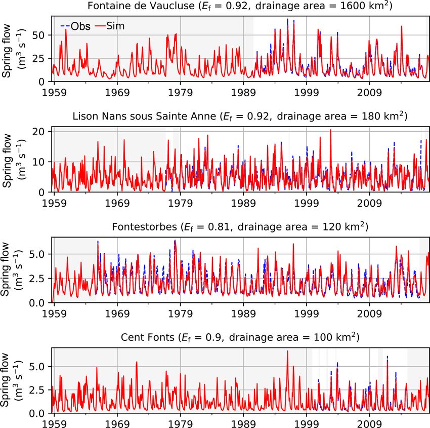
J.-P. Vergnes et al.: The AquiFR hydrometeorological modelling platform                                                          635

al., 2015) and forecast (Singla et al., 2012; Thirel et al., 2010)   simulation provides a unique insight on the long-term evolu-
includes an explicit representation of two aquifer systems.          tion of groundwater in France, as most of the groundwater
However, the representation of these aquifer systems is rather       data are available over about 30 years. This long-term sim-
coarse and is mostly used to have a realistic representation of      ulation can then be used to characterize the daily situation
the river base flow (Rousset et al., 2004) rather than provide       compared to past events. A wide range of gauging stations
consistent information on groundwater resources. Vergnes et          and piezometers were selected in order to perform the eval-
al. (2012) developed a hydrogeological model dedicated to            uation of the simulated piezometric heads, river flows and
climate modelling that was first applied over France and on a        karstic spring flows. This evaluation allows for identifying
global scale (Vergnes and Decharme, 2012). However, only             extreme events such as groundwater floods or droughts over
a single layer at the resolution of approximately 10 km over         a long-term period. In this paper, a detailed description of the
France was considered. This approach is still too coarse to be       AquiFR platform and its components is presented in Sect. 2.
used for groundwater management over France.                         Section 3 provides information on the regional models, their
   The need to have a national-scale consistent representation       calibration and the statistical criteria used to evaluate their
of groundwater resources in France clearly appeared during           performance. Section 4 presents the assessment of the long-
the project Explore 2070 led by the French environment min-          term simulation based on a comparison with observations of
istry that aimed at providing climate projections of the evo-        river flows, karstic spring flows and piezometric heads. The
lution of water resources in France including groundwater            results are then discussed in Sect. 5, prior to the conclusions.
(Stollsteiner, 2012). Several regional hydrogeological mod-
els were used in this project, together with downscaled cli-
mate change projections. The results were difficult to analyse       2   The AquiFR hydrometeorological modelling
due to the differences in the way the surface water balance              platform
was calculated (either a lumped-parameter model or soil–
vegetation–atmosphere scheme), in the initialization meth-           The AquiFR hydrometeorological modelling platform rep-
ods and in the way the models estimated the evolutions.              resents the main hydrological processes occurring within
Moreover, in the meantime, several regional groundwater              the watersheds from precipitations to groundwater flows
models were developed independently by research institu-             as shown in Fig. 1. In its present form, the AquiFR sys-
tions in a close relationship with the stakeholders for regional     tem includes three hydrogeological modelling software pro-
water management purposes or climate impact studies (Am-             grammes covering 11 sedimentary aquifers and 23 karstic
raoui et al., 2014; Croiset et al., 2013; Douez, 2015; Habets        systems: the EauDyssée hydro(geo-)logical numerical plat-
et al., 2010; Monteil et al., 2010; Vergnes and Habets, 2018).       form (Saleh et al., 2013), the MARTHE (Modélisation
   In such a context, the AquiFR project was initiated to cap-       d’Aquifères avec un maillage Rectangulaire, Transport et
italize on these developments in order to provide real-time          HydrodynamiquE; Modelling Aquifers with Rectangular
monitoring (Coustau et al., 2015) and forecasts (Singla et           cells, Transport and Hydrodynamics) groundwater flow soft-
al., 2012; Thirel et al., 2010) of groundwater resources in          ware programme (Thiéry, 2015a) and the EROS (Ensem-
France, as well as long-term reanalyses and future projec-           ble de Rivières Organisés en Sous-bassins; set of rivers or-
tions. The project associates research teams in hydrogeo-            ganized in sub-basins) lumped model software programme
logical, numerical-modelling and atmospheric fields. A na-           used for karstic systems (Thiéry, 2018a). These software pro-
tional stakeholder in charge of the water resource, the French       grammes are embedded in an application developed with the
Agency for Biodiversity (AFB), funds this project. The main          OpenPALM (Projet d’Assimilation par Logiciel Multimeth-
idea of AquiFR is to include existing hydrogeological mod-           odes) coupling system (Duchaine et al., 2015). All of these
els developed with different groundwater modelling software          models cover an area of about 149 000 km2 and contain up to
programmes and to connect them with real-time atmospheric            10 overlaid aquifer layers.
analysis and weather forecasts for producing relevant infor-            AquiFR accounts for spatial heterogeneity by using dif-
mation for water resource management through a single nu-            ferent spatial scales. The SAFRAN meteorological analy-
merical tool. This project also encourages new developments          sis (Quintana-Seguí et al., 2008; Vidal et al., 2010), avail-
over areas where no groundwater models currently exist. To           able over the French metropolitan area at an 8 km resolution,
achieve these objectives the AquiFR hydrogeological mod-             supplies the meteorological variables to the SURFEX (SUR-
elling platform was developed. The main objectives of this           Face EXternalisée) land surface model (Masson et al., 2013),
paper are to describe this platform, to evaluate its perfor-         which evaluates the water balance over the French metropoli-
mance against observations, and to prove its suitability and         tan area. SAFRAN provides hourly precipitation (rainfall and
robustness for operational and research purposes.                    snowfall), temperature, relative air humidity, wind speed and
   Prior to real-time monitoring and forecast, AquiFR needs          downward radiation. SURFEX uses these atmospheric vari-
to be assessed over a long-term period, which is presented in        ables to solve the energy and surface water budget at the
the present study. The evaluation is carried out over a 60-year      land–atmosphere interface at a 5 min time step. SURFEX
period from 1958 to 2018 at a daily time step. This long-term        estimates the spatial partition of the flow between surface

www.hydrol-earth-syst-sci.net/24/633/2020/                                           Hydrol. Earth Syst. Sci., 24, 633–654, 2020
636                                                   J.-P. Vergnes et al.: The AquiFR hydrometeorological modelling platform

Figure 1. Scheme of the AquiFR physical system. The simulation of the watersheds depends on its hydrogeologic characteristics. For sedi-
mentary basins, the transfer of water within the watersheds is estimated by MARTHE or EauDyssée. It accounts for flows in the unsaturated
zones, to (red thin arrow) and in the rivers, in (black arrows) and between (blue arrows) aquifer layers, as well as the exchange between the
river and the aquifer (purple arrow). The temporal resolution is daily, and the spatial resolution varies from 100 m to a maximum of 8000 m.
The depth of the deepest aquifer layer can locally reach about 1000 m. The 8 km spatial partition of the flow between surface runoff and
groundwater recharge (red thick arrows) is estimated by the SURFEX land surface scheme. It solves the water and energy budget at a 5 min
time step. It accounts for the local type of vegetation and soil, the presence of snow, and a multilayer soil that can reach a depth of 3 m. The
atmospheric forcing is provided by SAFRAN. For the karstic systems, the EROS conceptual model is used. It represents each karstic system
as lumped basins based on a reservoir approach at a daily timescale. The incoming atmospheric forcing is provided by SAFRAN.

runoff and groundwater recharge on the SAFRAN 8 km reso-                  can locally reach about 1000 m. It must be stressed that the
lution grid. It accounts for different soil and vegetation types          hydrogeological models could have been classically fed with
and uses a diffusion scheme to represent the transfer of heat             the SAFRAN analysis precipitation, potential evapotranspi-
and water through the soil. The soil in SURFEX is repre-                  ration and temperature data using their own water balance
sented by a multilayer approach. Its depth varies according to            calculation. However, the combined use of SURFEX and
the vegetation (in France from 0.2 to 3 m) and is partly acces-           SAFRAN provides a consistent set of hydro-meteorological
sible to plant roots. Deep soil infiltration constitutes ground-          data over an 8 km resolution grid over France, including
water recharge flux. Surface runoff can occur according to                groundwater recharge and surface runoff from SURFEX, as
saturation excess or infiltration excess.                                 well as potential evapotranspiration, precipitation and tem-
   The simulation of the watersheds depends on its hydro-                 perature from SAFRAN. The use of these SURFEX 8 km
geologic characteristics. For sedimentary basins, these two               resolution fluxes made the recalibration of the hydrogeologi-
fluxes are transferred to the MARTHE (Thiéry, 2015a) or                   cal models included in the platform necessary.
EauDyssée (Saleh et al., 2013) groundwater models. These                     Karstic aquifer systems are simulated through a concep-
models simulate the transfer to the unsaturated zone, ground-             tual reservoir modelling approach using the EROS soft-
water flows within and between the aquifer layers, the rout-              ware programme (Thiéry, 2018a). Each karstic system is
ing of surface runoff to and within rivers, and river–aquifer             represented by a lumped reservoir model solved at a daily
exchanges. They also account for the numerous groundwa-                   timescale. Conceptual approaches are preferred for simulat-
ter abstractions within the river basins. The temporal resolu-            ing karstic systems. Indeed, their heterogeneities make it dif-
tion is daily, and the spatial resolution varies from 100 m to a          ficult to use a physically based approach. EROS uses the
maximum of 8000 m. The depth of the deepest aquifer layer                 daily precipitation, snow, temperature and potential evap-

Hydrol. Earth Syst. Sci., 24, 633–654, 2020                                                www.hydrol-earth-syst-sci.net/24/633/2020/
J.-P. Vergnes et al.: The AquiFR hydrometeorological modelling platform                                                         637

otranspiration provided by SAFRAN to compute karstic                simulations. Originally intended for mountainous areas, it
spring flows.                                                       was later extended to cover France (Quintana-Seguí et al.,
   Technically, the AquiFR hydrogeological modelling plat-          2008). SAFRAN estimates eight variables: rainfall, snow-
form was developed using the OpenPALM coupling system               fall, incoming solar and atmospheric radiation, cloudiness,
(Buis et al., 2005; Duchaine et al., 2015). OpenPALM al-            air temperature and relative humidity 2 m above ground, and
lows for the easy integration of high-performance computing         wind speed at 10 m. Potential evapotranspiration can also
applications in a flexible and scalable way. It was originally      be computed from these atmospheric variables. SAFRAN
designed for oceanographic data assimilation algorithms, but        is based on climatic zones where the atmospheric variables
its application domain extends to multiple scientific applica-      only vary according to the topography. More than 600 homo-
tions. In the framework of OpenPALM, applications are split         geneous climate zones are defined over France. The average
into elementary components that can exchange data. The              area for each zone is about 1000 km2 so that each one con-
AquiFR platform is an OpenPALM application that currently           tains one surface meteorological station and at least two rain
gathers five components. Figure 2 shows the linkage between         gauges. SAFRAN uses all the observations available to esti-
these components and the workflow of an AquiFR run. In              mate each atmospheric variable except for radiation. For each
version 1.2 of AquiFR, no feedback from groundwater to the          variable, values are assigned to given altitudes using an opti-
soil of SURFEX is taken into account. Therefore, a prelimi-         mal interpolation method. The analyses are computed every
nary step illustrated by Fig. 2a is carried out in order to esti-   6 h, and an interpolation is made to an hourly time step. Radi-
mate groundwater recharge and surface runoff with SURFEX            ation fluxes are computed using a radiative transfer scheme.
accounting for the atmospheric forcing from SAFRAN prior            The daily precipitation rates are estimated using a wide range
to an OpenPALM run. This preliminary step gives access to           of daily rain gauges and converted to hourly data using the
60 years of daily groundwater recharge and surface runoff           evolution of the relative air humidity. The vertical profiles of
on a regular 8 km resolution over all the French metropolitan       the atmospheric parameters are then computed in each cli-
area.                                                               matic zone, and the values are spatially interpolated over the
   These water fluxes are then accessible by the OpenPALM           8 km grid as a function of the altitude within each climatic
application that includes the three hydrogeological mod-            zone. Further details on the SAFRAN analysis system can be
elling components, the pre-processing component and the             found in Quintana-Seguí et al. (2008) and Vidal et al. (2010).
post-processing component as shown in Fig. 2b. All of these
components exchange data during the parallel execution of           2.2   The SURFEX modelling platform
a single OpenPALM run. At each daily time step, a first pre-
processing component retrieves both the atmospheric forcing         SURFEX is a modelling platform aimed at simulating the
and the SURFEX groundwater recharge and surface runoff              water and energy fluxes at the interface between the sur-
at the beginning of the time step. Then, the EauDyssée,             face and the atmosphere (Masson et al., 2013). SURFEX
MARTHE and EROS modelling software programmes com-                  is built to be coupled to forecast and climate models. It in-
pute the evolution of the simulated hydrogeological variables       cludes databases, interpolation schemes and several physical
for the current time step for each groundwater model inde-          options that allow its use over different spatial and temporal
pendently. A last post-processing component synchronizes            scales. SURFEX gathers several physical schemes in a single
the simulation (it waits until all the models have ended their      platform, allowing for the simulation of the urban surfaces
computations for the current time step) and collects the in-        and the main components of the water cycle: sea and ocean,
dividual outputs of each model to write to comprehensive            lake, vegetation, and soil.
outputs for the entire domain. At last, a signal is sent by the        Land surface processes are taken into account using the In-
post-processing component in order to allow the platform to         teraction between Soil, Biosphere, and Atmosphere (Noilhan
compute the next time step. The use of OpenPALM allows              and Planton, 1989) land surface scheme. ISBA uses a short
for running each instance of the models in parallel on several      list of parameters depending on vegetation and soil types.
processors. The 60-year simulation presented in this study          The temporal evolution of the soil water and energy budget
needs approximately 1.5 d of computation time on a high-            is computed using a multilayer soil scheme based on the ex-
performance computer. The following subsections present             plicit resolution of the one-dimension Fourier law as well as
a brief description of the components integrated within the         the mixed form of the Richards equation (Boone et al., 2000;
OpenPALM application in AquiFR.                                     Decharme et al., 2013). Groundwater–surface-water capil-
                                                                    lary exchanges can be explicitly taken into account (Vergnes
2.1   The SAFRAN meteorological analysis                            et al., 2014) as well as the vertical root profile in the soil
                                                                    (Braud et al., 2005).
The SAFRAN meteorological analysis is a mesoscale atmo-                In the present study, no bidirectional coupling between the
spheric analysis system for surface variables. It provides me-      soil of SURFEX and the aquifers is accounted for. Thus, a
teorological forcing data over France on an 8 by 8 km grid          one-way coupling from the soil of SURFEX to the aquifer is
at the hourly time step using observed data and atmospheric         taken into account in order to provide groundwater recharge

www.hydrol-earth-syst-sci.net/24/633/2020/                                          Hydrol. Earth Syst. Sci., 24, 633–654, 2020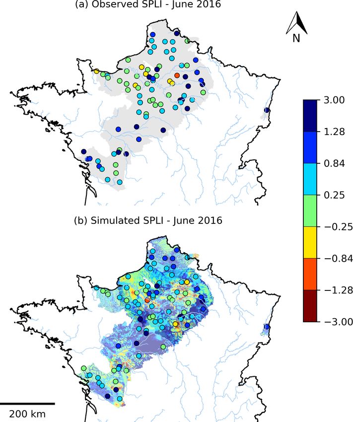
638                                                   J.-P. Vergnes et al.: The AquiFR hydrometeorological modelling platform

Figure 2. Scheme of the numerical implementation of AquiFR. (a) SAFRAN and SURFEX are run separately, as well as the processes
that extract the daily surface runoff and groundwater recharge at 8 km resolution on a daily time step over the full 60-year period. (b) The
components implemented within the OpenPALM (O-Palm) coupling system are presented. Pre-processing in blue gives access to the surface
runoff and groundwater recharge as well as atmospheric forcing to the three groundwater models for the current time steps. Then, each
hydrogeologic software programme runs all of their models for the current time step. The fluxes and state variables are then transferred daily
to post-processing that writes the model outputs and manages the following time step.

and surface runoff to the AquiFR platform. The soil column               2.3    The EauDyssée groundwater modelling software
thickness represented in each 8 km resolution grid cell varies                  programme
from 0.20 to 3 m according to the land cover. It corresponds
mostly to the root zone layer (Decharme et al., 2013). Thus,             The EauDyssée modelling platform gathers numerical mod-
the recharge provided by SURFEX is the vertical flux leaving             ules representing several hydrological processes, the most
the bottom of the soil column of each grid cell. Further details         important being the aquifer module based on the Simulation
on ISBA can be found in Decharme et al. (2013).                          des Aquifères Multicouches (SAM; multilayer aquifer sys-
                                                                         tem) regional groundwater modelling software programme
                                                                         (Ledoux et al., 1989) and the river routing scheme based
                                                                         on the Routing Application for Parallel computatIon of Dis-
                                                                         charge (RAPID) model (David et al., 2011).
                                                                            SAM computes the evolution of the piezometric heads
                                                                         of multilayer aquifers using a finite difference numerical

Hydrol. Earth Syst. Sci., 24, 633–654, 2020                                               www.hydrol-earth-syst-sci.net/24/633/2020/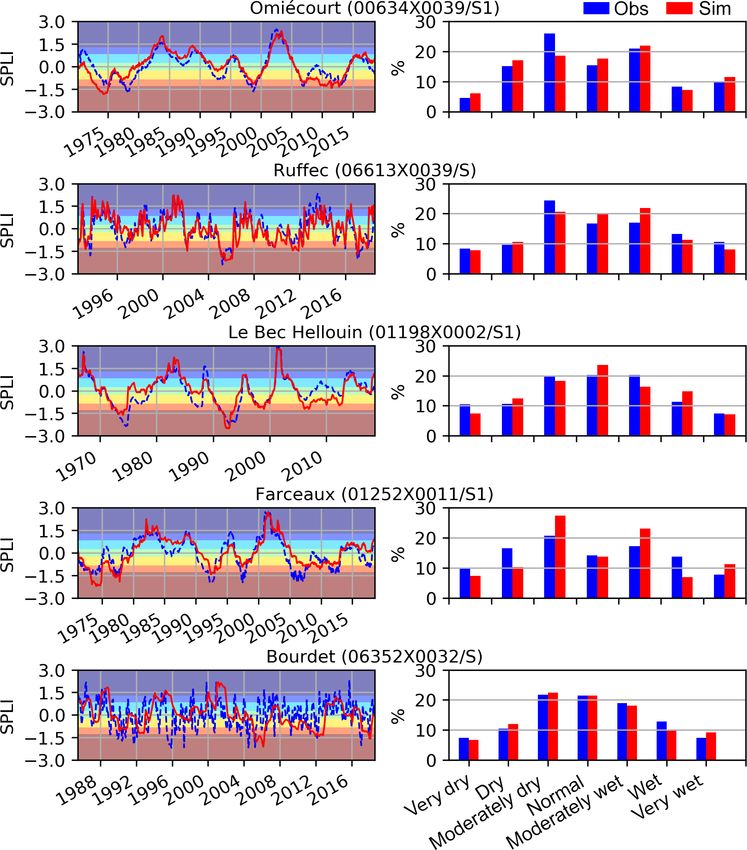
J.-P. Vergnes et al.: The AquiFR hydrometeorological modelling platform 639
scheme to solve the groundwater diffusivity equation with a 2.5 The EROS software programme
square grid discretization. Groundwater horizontal flows are
2-dimensional, and vertical flows through aquitards are taken The Ensemble de Rivières Organisés en Sous-bassins (set
into account. Therefore, unconfined and confined aquifers of rivers organized in sub-basins) numerical code is a dis-
can be represented. SAM was successfully used to predict tributed reservoir modelling software programme dedicated
groundwater and surface water flows in different basins of to large river systems (Thiéry, 2018a; Thiéry and Mout-
various scales and hydrogeological contexts: the Seine basin zopoulos, 1992). It allows the simulation of river flow or
(Viennot, 2009), the Somme basin (Habets et al., 2010), karstic spring flow and piezometric-head measurements in
the Loire basin (Monteil et al., 2010) or the Rhine basin heterogeneous river basins. These river basins are repre-
(Thierion et al., 2012; Vergnes and Habets, 2018). sented in EROS as a cluster of elementary lumped-parameter
The RAPID software programme is a river routing model hydrological models connected with each other. For each
based on the Muskingum routing scheme (David et al., sub-model, a hydroclimatic lumped model computes the lo-
2011). It can be coupled to groundwater and land surface cal river discharge at the outlet of the sub-model and the
models. Volumes and river flows are computed along a river piezometric head in the underlying water table. Each sub-
network discretized into square grid cells to ease the simula- model simulates the main mechanisms of the water cycle
tion of the exchanges with groundwater. River–groundwater through simplified physical laws (Thiéry, 2015d). Snow ac-
exchanges are taken into account in both directions. cumulation, snow melting and pumping are taken into ac-
count. The total river flow at the outlet of each sub-basin is
2.4 The MARTHE groundwater modelling software computed from the upstream tree of sub-basins.
programme EROS was initially developed to simulate regional wa-
tersheds avoiding the complexity of a spatially and physi-
The Modélisation d’Aquifères avec un maillage Rectangu- cally based model. In the framework of AquiFR, this soft-
laire, Transport et HydrodynamiquE (Modelling Aquifers ware programme was adapted in order to simulate in a sin-
with Rectangular cells, Transport and Hydrodynamics) com- gle instance 23 karstic systems as independent sub-models
puter code is the hydrogeological modelling software pro- (Thiéry, 2018b). It is not connected to SURFEX but directly
gramme from the French Geological Survey (BRGM) to SAFRAN as described in Fig. 1.
(Thiéry, 2015a, b, c). MARTHE embeds single-layer to mul-
tilayer aquifers and hydrographic networks. It is designed for
2-dimensional or 3-dimensional modelling of flows and mass
3 Methodology
transfers in aquifer systems, including climatic, human influ-
ences and possible geochemical reactions. Groundwater flow 3.1 The regional models implemented in the AquiFR
is computed by a 3-dimensional finite volume approach to platform
solve the hydrodynamic equation based on Darcy’s law and
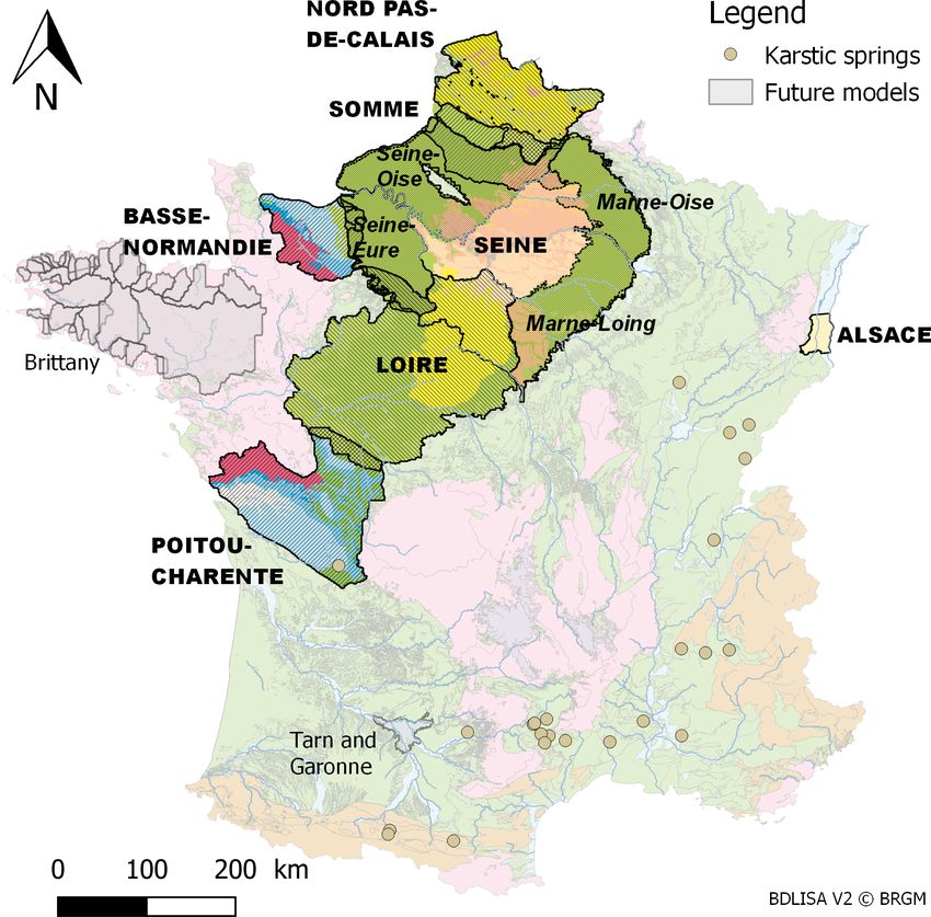
mass conservation, using irregular rectangular grids, with the AquiFR aims at covering all groundwater resources in
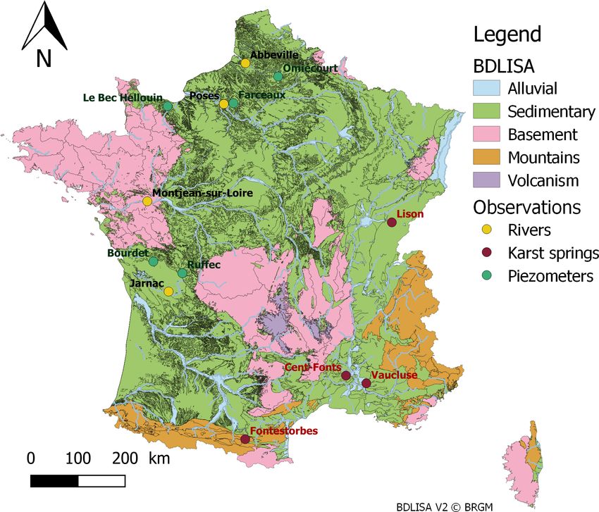
possibility of nested grids. River flows are simulated based France. Figure 3 shows the main aquifers covering France
on a kinematic wave approach that is fully coupled to ground- classified by geological type as defined in the French hy-
water flow. Groundwater–river exchanges are taken into ac- drogeological reference system Base de Donnée des Limites
count in both directions. des Systèmes Aquifères (BDLISA; https://bdlisa.eaufrance.
Other options are available and can be integrated into the fr/, last access: 11 February 2020). The current version of
simulation: mass transfer for pollutants in water, temperature AquiFR gathers 13 spatially distributed models correspond-
effects, impact of salinity, degradation of pollutants, transfers ing to regional single-layer or multilayer aquifers (Table 1
in the unsaturated zone and geochemical reactions. and Fig. 4).
This software programme is widely used for groundwater Some regions are simulated by two spatialized models
resources management in France: for example in the Somme (Fig. 4): the Somme and the Basse-Normandie basins are
River basin (Amraoui et al., 2014), in the Poitou-Charentes covered by the MARTHE and EauDyssée models, and the
region (Douez, 2015), in the Basse-Normandie (Lower Nor- chalk aquifer of the Seine basin is covered by both the
mandy) region (Croiset et al., 2013) or in the Aquitaine sed- EauDyssée Seine model and four EauDyssée sub-models
imentary basin (Saltel et al., 2016). It is also used in other (Marne–Loing, Marne–Oise, Seine–Eure and Seine–Oise re-
environmental fields such as pollutant infiltration in unsatu- gional models; see Fig. 4). This allows for a multi-model ap-
rated zones (Herbst et al., 2005; Thiéry et al., 2018) or for the proach, which can be useful for forecast and climate change
simulation of pollution plume coming from a contaminated impact studies. For these regions, the results presented in this
area. paper correspond to the models that were considered as the
best calibrated with the SURFEX fluxes. It corresponds to
the four EauDyssée sub-models over the Seine basin and the
Somme and Basse Normandie MARTHE models. Figure 4
www.hydrol-earth-syst-sci.net/24/633/2020/ Hydrol. Earth Syst. Sci., 24, 633–654, 2020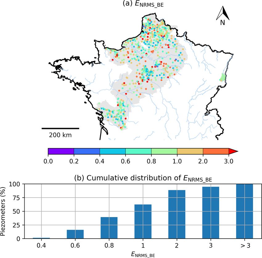
640                                                   J.-P. Vergnes et al.: The AquiFR hydrometeorological modelling platform

Figure 3. Main aquifers of France classified by geological type from the BDLISA version 2 database (https://bdlisa.eaufrance.fr/, last access:
11 February 2020). The names of the gauging stations and piezometers shown in Figs. 8, 12 and 13 are written.

Table 1. Short description of the regional multilayer aquifer models available in AquiFR. Periods of calibration are given in the Recalibration
column, and the type of variables used for recalibration are in the Variables column. GW means groundwater level, and RF is river flow.
GW levels were evaluated using RMSE and bias criteria. River flows were evaluated using Ef and the ratio criteria.

           Software       Model                  Number      Number      References                     Recalibration    Variables
                                                 of layers   of cells
                          Basse-Normandie                4     37 667    Thierion (2007)                1986–2013        GW
                          Loire                          3     37 620    Monteil et al. (2010)          No
                          Marne–Loing                    4     66 235    Viennot and Abasq (2013)       1996–2015        GW
                          Marne–Oise                     2     45 904    Viennot and Abasq (2013)       1986–2015        GW
           EauDyssée
                          Seine                          6     41 609    Viennot (2009)                 Not necessary    GW
                          Seine–Eure                     1     57 306    Viennot and Abasq (2013)       In progress
                          Seine–Oise                     4     87 178    Viennot and Abasq (2013)       1996–2015        GW
                          Somme                          1     63 226    Korkmaz (2007)                 No
                          Alsace                        3      40 947    Noyer and Elsass (2006)        No
                          Basse-Normandie              10      93 800    Croiset et al. (2013)          No
           MARTHE         Nord Pas-de-Calais           10     226 077    Bessière et al. (2015)         1995–2009        GW, RF
                          Poitou-Charentes              8      90 084    Douez (2015)                   Not necessary    GW, RF
                          Somme                         1      66 924    Amraoui et al. (2014)          1989–2012        GW, RF

also shows the 23 karstic systems (median catchment area of                 Groundwater withdrawals are integrated as time-
99 km2 ) simulated by EROS (Thiéry, 2018b) as well as the                 dependent boundary conditions in the spatially distributed
hard-rock aquifer in Brittany that will be simulated using a              models. On annual average and with respect to the total
hillslope model (Courtois, 2018; Marçais et al., 2017) and                surface area of the simulated domain, it corresponds to about
integrated in the near future.                                            16 mm yr−1 (2.4 billion of cubic metres per year) distributed

Hydrol. Earth Syst. Sci., 24, 633–654, 2020                                               www.hydrol-earth-syst-sci.net/24/633/2020/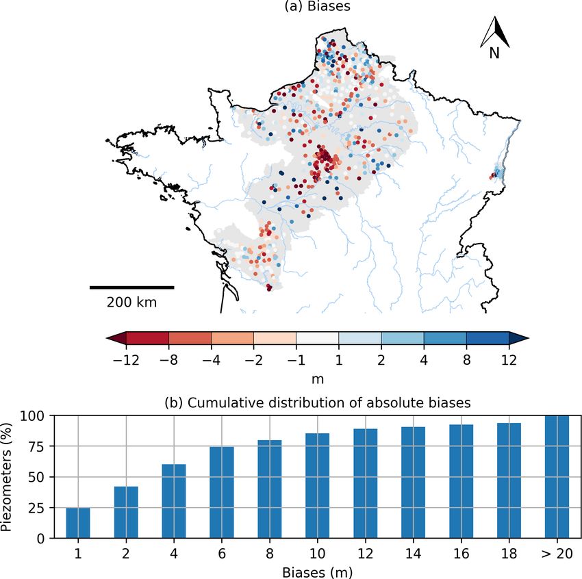
J.-P. Vergnes et al.: The AquiFR hydrometeorological modelling platform                                                           641

                                                                      based either on a lumped-parameter rainfall–runoff model in-
                                                                      tegrated in the MARTHE computer code or by the RAPID
                                                                      river routing model using a fine-scale river network covering
                                                                      all of France.

                                                                      3.2   Calibration of the hydrogeological models

                                                                      The original hydrogeological regional models were devel-
                                                                      oped independently, most often based on stakeholder re-
                                                                      quests. The water budgets were usually computed using
                                                                      less physical methods and atmospheric local data (precipita-
                                                                      tion, temperature and potential evapotranspiration) that dif-
                                                                      fer from the physically based approach using SURFEX and
                                                                      the SAFRAN analysis. As a result, in order to be consistent
                                                                      with the estimation of the groundwater recharge estimated
                                                                      by SAFRAN–SURFEX, most of the regional models were
                                                                      recalibrated based on new fluxes (Habets et al., 2017). This
                                                                      recalibration effort was not undertaken for the Alsace and
                                                                      Loire models, since both of them will be soon updated and
                                                                      then recalibrated.
Figure 4. Map of the regional multilayer aquifers and the karstic        Periods of recalibration were the same as those initially
systems simulated in AquiFR. The outlines of the models are also      used to develop and calibrate each model (see references in
shown with colours corresponding to the outcropping aquifers with     Table 1) in order to facilitate the comparison between the
respect to their geological contexts. Grey areas correspond to mod-   recalibrated models and the initial models. Hydrodynamic
els that will be integrated in the near future.                       parameters, including hydraulic conductivities and specific
                                                                      yields, were modified based on hydrogeological expertise in
                                                                      order to obtain the best fit between observations and simu-
in more than 16 000 grid cells. Data on groundwater pump-             lations. The calibration was made only on the piezometric
ing are provided by the regional water agencies based on              heads, except for the MARTHE Somme model for which
tax reporting. Pumping concerns drinking water, irrigation            piezometric heads and river flows were accounted for and
and industrial use. The quality of the dataset as well as its         for the karstic systems with karst spring flows only. All the
temporal extension varied for each regional model, although           models were recalibrated using the same statistical criteria.
the later does not exceed 20 years. Further details on regional       A comparison between the initial water budget of the mod-
models can be found in the references listed in Table 1. To           els and the SURFEX fluxes was performed as a first step to
extend the pumping estimation to the 1958–2018 period, a              estimate the need for recalibration of each model.
monthly mean annual cycle is defined for the years without               Some models, such as the Seine EauDyssée model, were
data. This choice is linked to the lack of knowledge about            not recalibrated since they perform equally well with the
past pumping. However, we do know that there have been                use of the SURFEX fluxes (see Table 1). In contrast, the
antagonistic developments between irrigation and industrial           MARTHE Somme River basin model was characterized by
pumping. Irrigation has increased in accordance with the              an excess of surface runoff in the north and a deficit in the
irrigated areas, while it varied greatly depending on the             south. In order to compensate for this imbalance, the total
climate. Industrial pumping was dominant in the past but has          runoff provided by SURFEX was split into surface runoff
considerably decreased during the past decades (Service de            and groundwater recharge using the original water balance
l’observation et des statistiques, 2016).                             scheme of MARTHE. This water balance scheme is based
   Each regional model uses its own river network at its own          on a reservoir for which parameters are calibrated in order
resolution. Most of the simulated domains encompass the en-           to compute the main components of the surface water budget
tire river basins corresponding to the simulated rivers. Only         (Thiéry, 2014). Only one reservoir was used, enabling a mod-
the Alsace and the Poitou-Charentes basins are partially rep-         ification of the partition of the total runoff and accounting for
resented. Therefore, they need to prescribe time-dependent            a delay on the groundwater recharge in order to mimic the
boundary conditions at the upstream of some rivers based on           impact of the deep unsaturated zone. It improved the simula-
river flow observations. If the observed data do not cover the        tion of the river flows using the SURFEX total runoff. Once
full period, the missing values are filled by the daily mean          the new partition was estimated, the aquifer permeability was
annual observed river flow. In the near future, the advan-            recalibrated. The Somme basin is the only one for which
tage to have the atmospheric forcing and surface fluxes over          only the total runoff from SURFEX was used. For the other
the entire domain will be used to estimate the upstream flow          basins, the estimation by SURFEX of the partition of the wa-

www.hydrol-earth-syst-sci.net/24/633/2020/                                            Hydrol. Earth Syst. Sci., 24, 633–654, 2020
642                                               J.-P. Vergnes et al.: The AquiFR hydrometeorological modelling platform

ter fluxes between surface runoff and groundwater recharge           observed and simulated river flows but can be used for other
was used. Overall, the performance of the models are similar         variables. Its use for comparing groundwater levels is less
with the original water balance fluxes and the ones simulated        obvious regarding its strong sensitivity to the biases between
by SAFRAN–SURFEX, although locally, they may be better               observation and simulation. It is equal to 1 when the model
or otherwise degraded.                                               perfectly fits the observations. An Ef criterion above 0.7 is
   For the karst system software programme EROS, the mod-            generally accepted as a good estimate of the signal dynamic,
els were calibrated based on the SAFRAN atmospheric anal-            depending however on the hydrogeological and climate con-
ysis by using an optimization of the statistical comparison          text of the basin. A negative Ef value means that the mean
between observed and simulated daily river flows.                    observed signal is a better predictor than the model. Ef is
   More information about the calibration is given in Habets         calculated as follows:
et al. (2017).                                                                  n
                                                                                       (Xobs (t) − Xsim (t))2
                                                                                P
3.3   Evaluation criteria of the 60-year simulation                             t=1
                                                                     Ef = 1 −     n                              ,              (3)
                                                                                  P                         2
Statistical criteria are used to evaluate the long-term simu-                             Xobs (t) − Xobs
lation. The bias B allows for an evaluation of the absolute                        t=1

mean deviation between the observation and the simulation.
                                                                     where Xobs is the temporal mean of observed values over the
It is calculated as follows:
          n
                                                                     considered period.
       1X                                                              The annual discharge ratio Rd criterion helps to compare
B=           (Xsim (t) − Xobs (t)) ,                       (1)
       n t=1                                                         the mean simulated and observed river flows as follows:
where n is the number of observed values and Xobs (t) and                   Qsim
Xsim (t) are the observed and simulated values respectively          Rd =          ,                                            (4)
                                                                            Qobs
at time t. B has the same unit as Xobs (t) and Xsim (t). The
perfect value is 0, while negative values correspond to under-       where Qsim and Qobs are the mean simulated and observed
estimation, and positive values correspond to overestimation.        river flows respectively.
   The root mean square error (RMSE) allows for an estima-              One way to evaluate the ability of the simulation to cap-
tion of the differences between the observed and simulated           ture extreme events is to use the standardized piezometric
values. It is often used to compare observed and simulated           level index (SPLI). The SPLI is an indicator used to compare
piezometric heads. However, the computation of the RMSE              groundwater level time series and to characterize the severity
is strongly affected by the biases. Therefore, we computed           of extreme events such as a long dry period or groundwa-
a RMSE bias-excluded value (ENRMS_BE ) in order to better            ter overflows (Seguin, 2015). It is currently used in France
assess the simulation in terms of amplitude and synchroniza-         for the Monthly Hydrological Survey (MHS) (Office Inter-
tion. Moreover, this RMSE bias-excluded value is normed              national de l’Eau, 2019). The MHS provides monthly infor-
with respect to the observed standard deviation for each ob-         mation to policymakers and the public on the hydrological
servation in order to account for the differences of variability     state of groundwater. Assessing the ability of the AquiFR
between the numerous wells to help spatial comparison or             modelling platform to reproduce this indicator is important
aggregation. This normed RMSE bias-excluded value is ex-             since the main objective of this platform is to predict such
pressed as follows:                                                  extreme events in short-to-long-term hydrogeological fore-
              1                                                      casts for groundwater management. The SPLI indicator is
ENRMS_BE =
             σobs                                                    based on the same principles as the standardized precipita-
                                                                     tion index (SPI) defined by McKee et al. (1993) to char-
             v
             u n
             uP                                     2
             u     Xsim (t) − Xsim − Xobs (t) − Xobs                 acterize meteorological drought at several timescales. First,
             t t=1
                                                           ,   (2)   monthly mean time series are computed from time series of
                                   n
                                                                     piezometric heads. Then, 12-monthly time series (January
where Xsim is the temporal mean of simulated values over             to December) are constituted over the N years of the time
the considered period and σobs is the observed standard de-          series period. For each time series of N monthly values, a
viation. The ENRMS_BE criterion is always positive and starts        non-parametric kernel density estimator allows for estimat-
from 0 for a perfect simulation of the observed amplitudes.          ing the best probability density function fitting the histogram
An ENRMS_BE criterion lower than 0.8 can be considered as            of monthly values. At last, for each month from January to
a reasonable estimation of the temporal evolution of the ob-         December, a projection over the standardized normal distri-
served water table.                                                  bution using a quantile–quantile projection allows for deduc-
   The Nash–Sutcliffe efficiency (NSE) coefficient Ef (Nash          ing the SPLI for each value of the monthly mean time se-
and Sutcliffe, 1970) measures the variance between the ob-           ries of piezometric heads. The SPLI values most often range
served and simulated values. It is often applied to compare          from −3 (extremely low groundwater levels corresponding to

Hydrol. Earth Syst. Sci., 24, 633–654, 2020                                              www.hydrol-earth-syst-sci.net/24/633/2020/
J.-P. Vergnes et al.: The AquiFR hydrometeorological modelling platform 643
Figure 5. Temporal evolution of the number of piezometric-head
measurements per day among the 639 selected piezometers over the
1958–2018 simulated period.
a return period of 740 years) to +3 (extremely high ground-
water levels). The SPLI allows for representing wetter and
drier periods in a similar way all over the simulated domain.
3.4 Dataset and model setup
The long-term simulation was carried out over a 60-year pe-
riod from 1 August 1958 to 31 July 2018 at a daily time
step using the SAFRAN meteorological analyses. State vari-
ables from 1 August 2013 were chosen from a first simu- Figure 6. (a) Spatial distribution of the biases calculated between
lation over the 1958–2018 period in order to initialize the the simulated and observed piezometric heads for the 639 selected
simulation on 1 August 1958. The year 2013 was chosen as piezometers. The grey background colour corresponds to the simu-
the best proxy of the year 1958 by analysing time series of lated aquifer domain. (b) Cumulative distribution of absolute biases
long-term observed groundwater levels with data since 1958. for all piezometers.
The mean precipitations corresponding to the simulated do-
main of Fig. 4 and averaged over the 60-year period is equal
to 743 mm yr−1 . SURFEX then computes the surface wa-
ter budget from the SAFRAN outputs. The mean simulated
total runoff is partitioned between 163 mm yr−1 of ground-
water recharge and 60.5 mm yr−1 of surface runoff. Thus,
the groundwater abstractions represent about 25 % of the
groundwater recharge.
The evaluation of this simulation is made using the numer-
ous in situ datasets available in France. Observed piezometric
heads are available in the Accès aux Données sur les Eaux
Souterraines (ADES) database (http://www.ades.eaufrance.
fr/, last access: 11 February 2020). A total of 639 observa-
tion boreholes covering the AquiFR domain corresponding
to both confined and unconfined aquifers, and with at least
10 years of continuous time series, were selected. Figure 5
shows the temporal evolution of the number of daily mea-
surements along the 60-year period. Starting in 1958, only
a few measurements are available. Starting from 1970, the
number of wells increases slowly to reach about 100 in 1990.
Then the number of daily measurements quickly increases to
reach more than 450 in 2010. This number remains stable
then, except for the last year (2018) where it decreases be- Figure 7. (a) Spatial distribution of ENRMS_BE calculated between
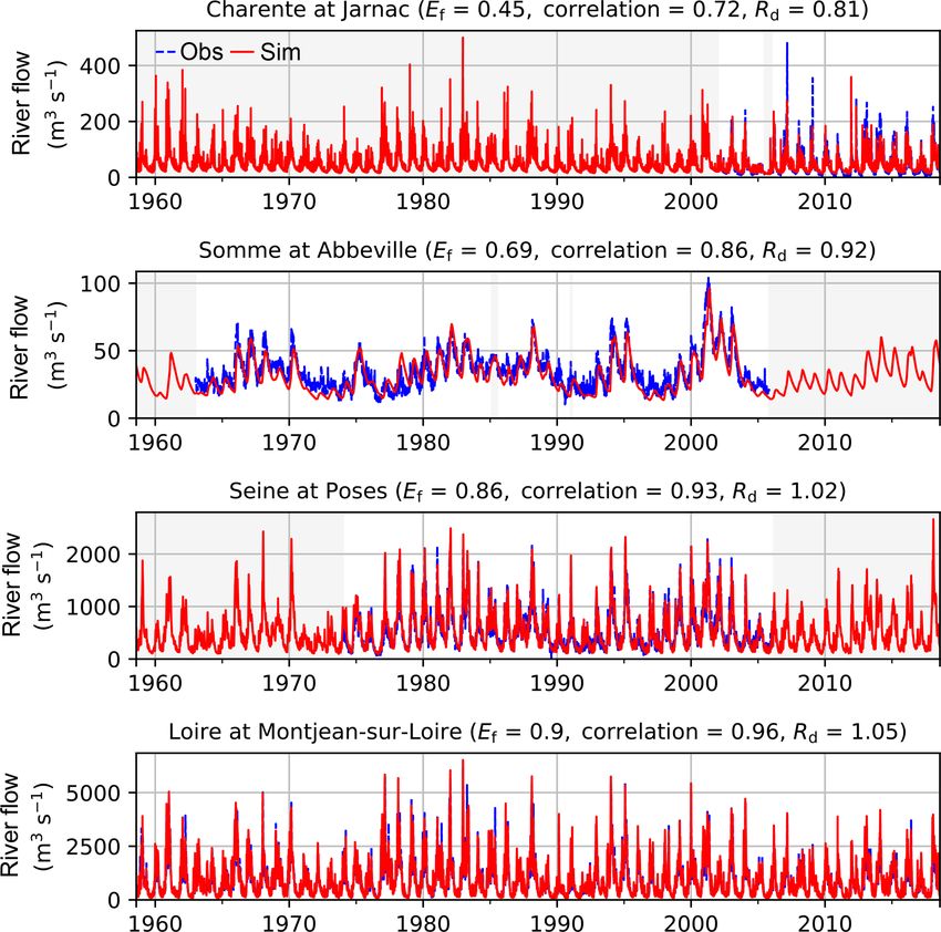
cause the datasets were not yet fully available. In situ daily the simulated and observed piezometric heads for the 639 selected
river flow observations at 362 gauging stations were also se- piezometers. The grey background colour corresponds to the simu-
lected for evaluating the daily simulated river flows from lated aquifer domain. (b) Cumulative distribution of ENRMS_BE for
all piezometers.
the Hydro database (http://hydro.eaufrance.fr/, last access:
11 February 2020).
www.hydrol-earth-syst-sci.net/24/633/2020/ Hydrol. Earth Syst. Sci., 24, 633–654, 2020644 J.-P. Vergnes et al.: The AquiFR hydrometeorological modelling platform
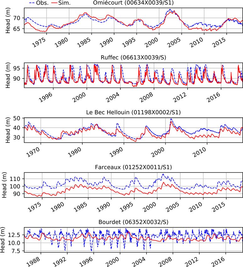
Figure 8. Daily observed (dotted blue) and simulated (red) piezometric-head variations for the five piezometers encircled in green in Fig. 3.
Table 2. Statistical scores of the comparison between the simulated and observed daily evolution of the piezometers shown in Fig. 8.
Piezometer Model Time series SPLI
ENRMS_BE Correlation Biases Ef Correlation
(m)
Omiécourt Somme 0.93 0.85 −0.86 0.73 0.87
Ruffec Poitou-Charentes 0.58 0.82 −1.44 0.6 0.79
Le Bec Hellouin Basse-Normandie 0.57 0.84 −2.76 0.73 0.86
Farceaux Seine–Oise 0.52 0.86 −8.34 0.67 0.84
Bourdet Poitou-Charentes 1.02 0.18 −0.72 −0.51 0.24
4 Results of the Loire River basin, corresponding to the Beauce region,
shows a significant underestimation of the mean observed
4.1 Piezometric head groundwater level. Elsewhere, no significant patterns appear.
Figure 6b summarizes these results with the cumulative dis-
Figure 6a shows the spatial distribution of the bias for tribution of the absolute biases for all the piezometers. A total
the 639 observed piezometers. A positive value means that of 42 % and 60 % of the absolute biases are lower than 2 and
the simulation overestimates the mean observed piezometric 4 m respectively.
head, while a negative value means the opposite. The north
Hydrol. Earth Syst. Sci., 24, 633–654, 2020 www.hydrol-earth-syst-sci.net/24/633/2020/J.-P. Vergnes et al.: The AquiFR hydrometeorological modelling platform 645
Figure 7 shows the spatial and cumulative distribution of
ENRMS_BE . A total of 16 %, 39 % and 62 % of the wells ob-
tain a value lower than 0.6, 0.8 and 1 respectively, while 88 %
have a value lower than 2. Some piezometers that were af-
fected by important biases in Fig. 6a however exhibit good
ENRMS_BE values, in particular over the Loire River basin
and in the northern Poitou-Charentes region, meaning that
the temporal evolution is well simulated.
Five examples of simulated and observed daily evolution
of piezometric heads are shown in Fig. 8. These piezometers
are encircled in Fig. 3, and statistical scores are available in
Table 2. They were chosen to characterize different hydroge-
ological contexts. The first piezometer named Omiécourt is
located in the chalk aquifer of the Somme River basin. The
temporal evolution of the groundwater level is characterized
Figure 9. Ef criterion calculated between the observed and simu-
by multiyear cycles well captured by the model. However,
lated SPLI for the 103 selected piezometers.
the simulation displays annual cycles that are not observed.
It explains why ENRMS_BE is equal to 0.93, while the bias is
equal to −0.86 m. The two piezometers named Ruffec and
Le Bec Hellouin correspond to limestone aquifers and are greater than 0.5, while 12 % are lower than 0. Figure 10 fo-
located in the Poitou-Charentes region and near the coast of cuses on five examples of observed and simulated temporal
the English Channel respectively. The first one is character- evolutions of the SPLI indicator. These piezometers corre-
ized by large annual cycles with wide amplitudes. The model spond to the ones shown in Fig. 8 and are part of the se-
is able to reproduce these annual cycles (correlation of 0.82) lected piezometers used for the MHS. Table 2 presents the re-
but with an underestimation of the peaks leading to a negative lated Ef and correlation scores. The Ef values computed for
bias of −1.44 m. The Le Bec Hellouin piezometer is charac- these SPLI time series are all greater than or equal to 0.6 ex-
terized by both multiyear and annual cycles that are captured cept for the Bourdet piezometer characterized by an Ef value
by the model, although between 2005 and 2015 the simu- equal to −0.51. This lower score may be due to a lack in the
lated groundwater level is underestimated with respect to the model input, such as the underestimation of withdrawal data
observation. The piezometer named Farceaux is located in in its vicinity.
a chalk aquifer in the Seine River basin. It is characterized The SPLI, as a frequency indicator, does not account for
by a systematic bias of about −8.3 m. Otherwise, the mul- the potential biases between the observed and simulated
tiyear and annual cycles are well reproduced by the model, groundwater levels. This is the reason why the systematic bi-
which is confirmed by the ENRMS_BE criterion equal to 0.52. ases found in Fig. 8 do not appear in the monthly SPLI com-
The last example corresponds to a piezometer for which the parisons in Fig. 10, in particular for the Farceaux piezometer.
model cannot reproduce the strong seasonal decrease of the The right part of Fig. 10 shows the histograms of the simu-
level occurring each year. Such behaviours in the observation lated (in red) and observed (in blue) monthly SPLI values for
are likely due to groundwater withdrawals that are not well each classes of Table 3. The histograms are similar for both
prescribed in the model near this well. the observed and simulated SPLI at the Ruffec and Le Bec
Hellouin piezometers. The occurrences of the wetter condi-
4.2 The standardized piezometric level index tions are well reproduced for the Omiécourt piezometer, but
the model tends to underestimate the number of moderately
The SPLI is categorized into seven classes summarized in dry conditions (26 % and 18 % events for the simulation and
Table 3 from the driest to the wettest conditions. According the observation respectively). For the Farceaux piezometer,
to Seguin and Klinka (2016), a set of piezometers were cho- the model underestimates the occurrences of the driest events
sen in order to compute the SPLI indicator in the MHS with and overestimates the occurrences of the wetter events. De-
the following characteristics: a continuous time series with spite the poor scores obtained for the Bourdet piezometer,
at least 15 years and no impact of pumping wells. Among in particular for the correlations, the distribution of all the
the 639 selected observation wells in Figs. 6 and 7, 103 con- monthly SPLI values with respect to the classes of Table 3 is
tribute to the MHS. similar for both the observation and the simulation.
Figure 9 shows the spatial distribution of Ef computed The MHS published every month in France for water re-
between the observed and simulated SPLI indicator for the source management includes the calculation of the SPLI.
103 selected piezometers. It assesses the ability of the model As an example, Fig. 11a shows the observed SPLI values
to reproduce the SPLI indicator in different locations. A total calculated for the 103 selected piezometers for June 2016.
of 20 % of the Ef values are greater than 0.7 %, and 56 % are We chose this specific month, since it follows large pre-
www.hydrol-earth-syst-sci.net/24/633/2020/ Hydrol. Earth Syst. Sci., 24, 633–654, 2020646 J.-P. Vergnes et al.: The AquiFR hydrometeorological modelling platform
Table 3. Classification of water table level classes related to the values of the SPLI corresponding to the MHS limits.
Classification SPLI values Return periods
Very low groundwater level < −1.28 > 10 dry years
Low groundwater level Between −1.28 and −0.84 Between 5 and 10 dry years
Moderately low groundwater level Between −0.84 and −0.25 Between 2.5 and 5 dry years
Normal groundwater level Between −0.25 and 0.25 Between 2.5 dry and 2.5 wet years
Moderately high groundwater level Between 0.25 and 0.84 Between 2.5 and 5 wet years
High groundwater level Between 0.84 and 1.28 Between 5 and 10 wet years
Very high groundwater level > 1.28 > 10 wet years
Figure 10. In the left panels are the monthly observed (dotted blue) and simulated (red) SPLI indicator variations for the five piezometers
encircled in green in Fig. 3. Font colours correspond to the classes of Table 3 from the driest (red) to the wettest (blue) intervals. In the right
panels are histograms in percentage of the SPLI values distributed against the classes of Table 3.
cipitation events that leads to floods in the Seine and Loire erately wet conditions: 19 % (29 %) of the simulated (ob-
basins (Philip et al., 2018). Figure 11b shows the simulated served) piezometers are in normal conditions; 46 % (31 %)
SPLI values computed for this specific month. The model are in moderately wet conditions; 16 % (13 %) are in wet
reproduces the overall pattern of normal and wet condi- conditions; and 16 % (18 %) are in extremely wet conditions.
tions but tends to overestimate the importance of the mod- The background map of Fig. 11b shows the SPLI computed
Hydrol. Earth Syst. Sci., 24, 633–654, 2020 www.hydrol-earth-syst-sci.net/24/633/2020/You can also read