Quantification of climate change impact on dam failure risk under hydrological scenarios: a case study from a Spanish dam
←
→
Page content transcription
If your browser does not render page correctly, please read the page content below
Nat. Hazards Earth Syst. Sci., 19, 2117–2139, 2019
https://doi.org/10.5194/nhess-19-2117-2019
© Author(s) 2019. This work is distributed under
the Creative Commons Attribution 4.0 License.

Quantification of climate change impact on dam failure risk under
hydrological scenarios: a case study from a Spanish dam
Javier Fluixá-Sanmartín1 , Adrián Morales-Torres2 , Ignacio Escuder-Bueno2,3 , and Javier Paredes-Arquiola3
1 Centrede Recherche sur l’Environnement Alpin (CREALP), Sion, 1951, Switzerland
2 iPresasRisk Analysis, Valencia, 46023, Spain
3 Research Institute of Water and Environmental Engineering (IIAMA),

Universitat Politècnica de València (UPV), Valencia, 46022, Spain

Correspondence: Javier Fluixá-Sanmartín (javier.fluixa@crealp.vs.ch)

Received: 11 May 2019 – Discussion started: 20 May 2019
Revised: 16 August 2019 – Accepted: 5 September 2019 – Published: 1 October 2019

Abstract. Dam safety is increasingly subjected to the influ-      1   Introduction
ence of climate change. Its impacts must be assessed through
the integration of the various effects acting on each aspect,     Dams are critical infrastructures whose associated failure
considering their interdependencies, rather than just a sim-      risk must be properly managed in a continuous and updated
ple accumulation of separate impacts. This serves as a dam        process (Fluixá-Sanmartín et al., 2018). When assessing their
safety management supporting tool to assess the vulnerabil-       safety levels, most dam risk assessments in the past assumed
ity of the dam to climate change and to define adaptation         a stationary condition in the variability of climate phenom-
strategies under an evolutive dam failure risk management         ena. However, climate change is likely to affect the different
framework.                                                        factors driving dam failure risks (USBR, 2014). The assump-
   This article presents a comprehensive quantitative assess-     tions of stationary climatic baselines are no longer appropri-
ment of the impacts of climate change on the safety of a          ate for long-term dam safety adaptation and decision-making
Spanish dam under hydrological scenarios, integrating the         support (USBR, 2016). Therefore, the way risk analyses are
various projected effects acting on each component of the         envisaged in the long term has to be revisited in order to in-
risk, from the input hydrology to the consequences of the         corporate the new climate change scenarios.
outflow hydrograph. In particular, the results of 21 regional        In this context, some efforts have been made in the evalu-
climate models encompassing three Representative Concen-          ation of climate change impacts on dam safety surveillance
tration Pathways (RCP2.6, RCP4.5 and RCP8.5) have been            (OFEV, 2014; USACE, 2014; USBR, 2014, 2016). However,
used to calculate the risk evolution of the dam until the end     the assessment of these impacts is usually applied separately
of the 21st century. Results show a progressive deterioration     and tends to focus on specific aspects such as the hydrolog-
of the dam failure risk, for most of the cases contemplated,      ical loads (Bahls and Holman, 2014; Chernet et al., 2014;
especially for the RCP2.6 and RCP4.5 scenarios. Moreover,         Novembre et al., 2015), relegating or ignoring other aspects.
the individual analysis of each risk component shows that the        The global effect of climate change on dam safety must be
alteration of the expected inflows has the greater influence on   quantitatively assessed through the integration of the various
the final risk. The approach followed in this paper can serve     projected effects acting on each aspect. In Fluixá-Sanmartín
as a useful guidebook for dam owners and dam safety practi-       et al. (2018), a dam safety management supporting tool is
tioners in the analysis of other study cases.                     defined to assess projected climate change impacts based on
                                                                  the risk analysis approach where all the variables concern-
                                                                  ing dam safety and their interdependencies could be included
                                                                  in a comprehensive way. In this context, risk analysis is a
                                                                  useful approach encompassing traditional and state-of-the-
                                                                  art methodologies to manage dam safety in an accountable

Published by Copernicus Publications on behalf of the European Geosciences Union.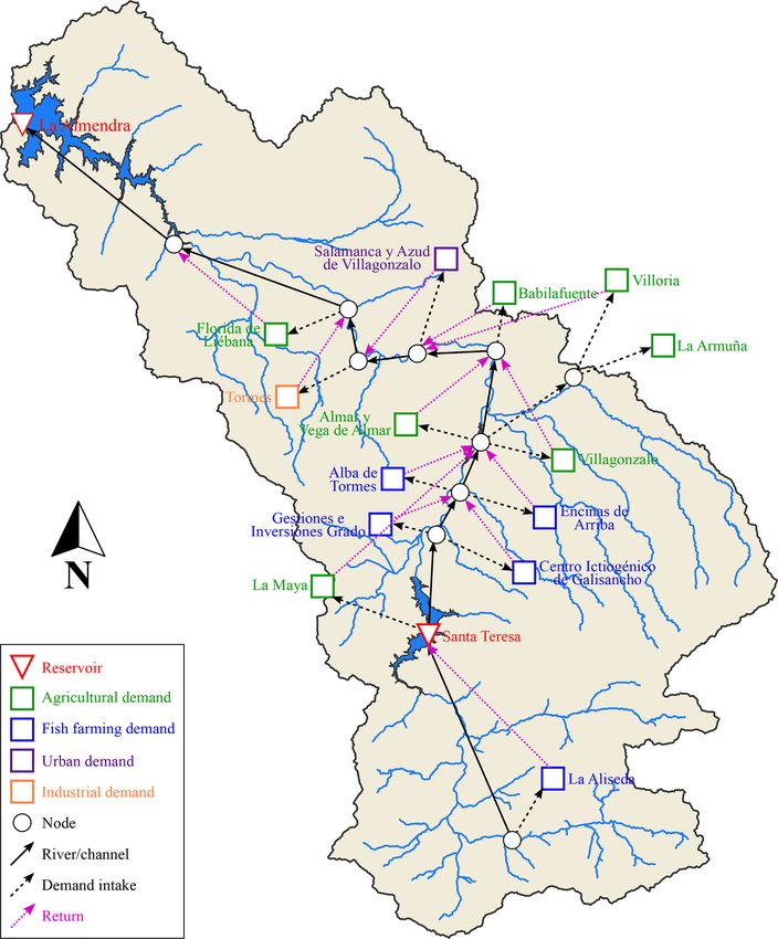
2118                                J. Fluixá-Sanmartín et al.: Quantification of climate change impact on dam failure risk

and comprehensive way (Bowles, 2000; Serrano-Lombillo               to both climatic and non-climatic drivers. This is based on
et al., 2013) that represents a useful basis on which such as-      the risk analysis approach where the effects on all the vari-
sessments can be structured. With this quantitative informa-        ables concerning dam safety – from the hydrological loads to
tion, long-term investments can be planned more efficiently,        the consequences of failure – and their interdependencies are
taking into account the potential evolution with time of risk       evaluated jointly. The cornerstone of the methodology is the
and the efficiency of measures.                                     application of a dam risk modelling approach which encom-
   In this work the authors seek a comprehensive quantitative       passes the information issued from different models and data
assessment of the climate change impacts on the failure risk        sources.
of a Spanish dam. The key innovative aspect of this method-            Moreover, since climate change is a non-stationary pro-
ology is the use of very different models and data sources,         cess, it is expected that its effects will change with time.
and their combination for the assessment of the overall ef-         Therefore, it is not only important to assess the global im-
fect of climate change in the resulting dam safety risk. The        pact of climate change on the dam failure risk but also how
analysis has been elaborated under hydrological scenarios,          this risk is expected to evolve with time. For this purpose,
where the floods are the main loads to which the dam is sub-        the methodology should be applied on the one hand to the
jected. In order to decompose such impacts on the different         present situation (to which the future results will be com-
risk aspects, a risk analysis scheme has been adopted. First,       pared) and on the other hand to different time horizons in the
the methodological approach proposed is presented. Then the         future. Given that the climate projections used in this study
study case of the Santa Teresa dam to which the methodol-           include results until the end of the 21st century, the following
ogy will be applied is described. The different data sources        four different periods are proposed in this study.
and existing models employed in this study are presented.
Using this information, the methodology is applied to the             – Historical: 1970–2005. It corresponds to the period for
study case, explaining the treatment of raw climate projec-             which hydro-meteorological observations are available,
tions, the elaboration of auxiliary models and the adaptation           as well as to the reference historical period of the cli-
of the risk model components. Finally, the output risks are             mate projections (see Sect. 4.2). This allows us to per-
presented and the resulting effects on the dam safety anal-             form the downscaling of the climate projections. Such a
ysed.                                                                   period will be referred to as the base case.

                                                                      – Period 1: 2010–2039.
2   Methodology
                                                                      – Period 2: 2040–2069.
This section describes the methodology proposed in this pa-
per for the calculation of climate change impacts on the              – Period 3: 2070–2099.
safety of dams. The goal is to analyse its effects on the differ-
ent dam failure risk components involved. It is worth noting           The methodology proposed is based on the following main
that, within the context of dam safety, failure risk can be de-     steps. A synthetic scheme of this methodology is presented
fined as the combination of three concepts: what can happen         in Fig. 1.
(dam failure), how likely it is to happen (failure probability),      a. Extraction and correction of climate projections.
and what its consequences are (failure consequences) (Ka-                First, the raw climate projections issued from the avail-
plan, 1997). Risk is obtained through the following formula:             able climate models must be bias-corrected using the
       X                                                                 climate observations. Assessing the impacts of climate
risk =     p(e) · p(f |e) · C(f |e),                          (1)
        e
                                                                         change on future runoff generation and on water re-
                                                                         source availability requires high-resolution climate sce-
where the risk is expressed in consequences per year (social             narios. Global climate models (GCMs) provide valuable
or economic), the summation is defined for all events e un-              prediction information but at a spatial resolution too
der study, p(e) is the probability of an event, p(f |e) is the           coarse (around 1000 km by 1000 km) to be directly used
probability of failure due to event e and C(f |e) represents             for modelling the hydrological processes at the required
the consequences produced as a result of each failure f and              scale (Akhtar et al., 2008; Fujihara et al., 2008; Or-
event e.                                                                 lowsky et al., 2008). Therefore, downscaling is required
   As stated in Fluixá-Sanmartín et al. (2018), changes in               to describe the consequences of climate change, which
climate such as variations in extreme temperatures or fre-               can be done using empirical–statistical downscaling or
quency of heavy precipitation events (IPCC, 2012; Walsh                  dynamical downscaling by means of regional climate
et al., 2014) are likely to affect the different risk compo-             models (RCMs). RCMs are commonly used in regional
nents driving dam failure. Hence, the proposed methodol-                 studies of climate projection and climate change im-
ogy intends to establish a framework for the evaluation of               pacts to downscale GCM simulations (Gao et al., 2006;
projected climate change impacts on dam safety attending                 Gu et al., 2012; Yira et al., 2017). They use the GCM

Nat. Hazards Earth Syst. Sci., 19, 2117–2139, 2019                          www.nat-hazards-earth-syst-sci.net/19/2117/2019/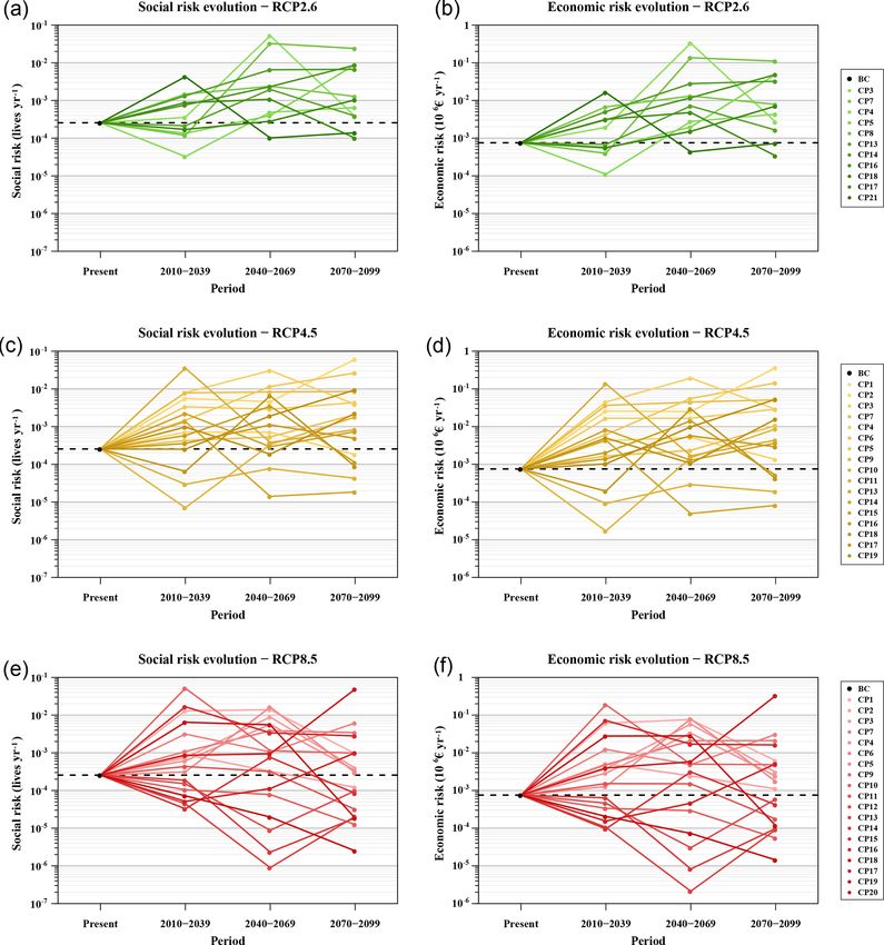
J. Fluixá-Sanmartín et al.: Quantification of climate change impact on dam failure risk 2119
outputs as lateral boundary conditions and thus their re-
sults depend to some extent on the driving GCM (Ben-
estad, 2016). However, the meteorological projections
issued from RCMs are usually biased and hence need to
be post processed before being used for climate impact
assessment (Gudmundsson et al., 2012).
b. Hydrological modelling. Then, a hydrological model is
set up based on the physical characteristics of the basin
and on the hydro-meteorological observations. On the
one hand, such a model allows us to perform the sim-
ulation of the system of water resources management
to obtain the relation between previous pool level and
probability at the reservoir, at the present situation and
for future scenarios. On the other hand, the hydrologi-
cal model is also used for the calculation of the flood
hydrographs arriving into the reservoir.
c. Risk modelling. The quantitative assessment of climate
change impacts on dam failure risk is conducted us-
ing a quantitative risk model of the dam. As explained,
such models are commonly used to inform dam safety
management and they integrate and connect most vari-
ables concerning dam failure risk to analyse the differ-
ent ways in which a dam can fail (failure modes) due to
a loading event, calculating their probabilities and con-
sequences (Ardiles et al., 2011; Serrano-Lombillo et al., Figure 1. Workflow of the methodology followed to assess climate
2011, 2012a, b; SPANCOLD, 2012). The model must change impacts on dam failure risk.
be adapted following the effects of climate change on
each of the risk components (Fluixá-Sanmartín et al.,
2018). relieving, altogether, 2050 m3 s−1 , as well as with two bot-
tom outlets with a release capacity of 88 m3 s−1 each. The
d. Correction of resulting risks. In order to consistently auxiliary dike is a 165 m long and 15 m high concrete gravity
assess and compare modelled risks, a change signal cor- dam with its crest level at 886.90 m a.s.l.
rection (likewise the delta change approach) must be The Santa Teresa reservoir has a capacity of 496 h m3 at its
applied to the results by scaling the outputs based on normal operating level (885.70 m a.s.l.). The catchment that
the difference between climate model and base case pours into the reservoir has a total surface of 1853 km2 and
risks for the historical reference period. This correction is part of the Tormes Water Exploitation System, with the
is computed as the relative variation between raw risk Santa Teresa reservoir being the first and uppermost infras-
output for a future scenario and risk of its correspond- tructure of the basin to regulate the Tormes River (Fig. 2).
ing historical reference period. Then, the future scenario The main uses for the Santa Teresa dam–reservoir system
risk is adjusted by multiplying this delta to the base case are hydropower production, flood protection, irrigation and
risk. water supply to the areas located between the Santa Teresa
and Almendra dams, including Salamanca city.
A risk analysis was already applied to the Santa Teresa
dam in a previous study (Ardiles et al., 2011; Morales-Torres
3 Study case et al., 2016). Results from this analysis showed that, although
the dam did not require urgent correction measures, its risk
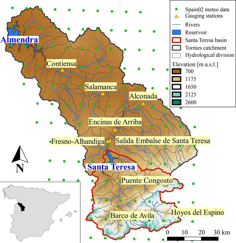
The Santa Teresa dam is located in the upper part of the
was important enough to be carefully monitored. Therefore,
Tormes River, in the province of Salamanca (Spain), and
it is interesting to evaluate whether its risk is expected to
is managed by the Duero River Basin Authority. The Santa
evolve up to the point of requiring correction measures.
Teresa reservoir is bounded by the Santa Teresa dam and a
smaller auxiliary dike. The Santa Teresa dam is a concrete
gravity dam built in 1960 and has a height of 60 m with
its crest level at 887.20 m a.s.l. and a length of 517 m. It is
equipped with a spillway regulated by five gates capable of
www.nat-hazards-earth-syst-sci.net/19/2117/2019/ Nat. Hazards Earth Syst. Sci., 19, 2117–2139, 2019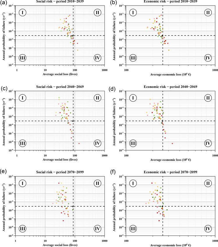
2120                                  J. Fluixá-Sanmartín et al.: Quantification of climate change impact on dam failure risk

                                                                        Santa Teresa reservoir from 1958 to 2015 is also available in
                                                                        this same platform.

                                                                        4.2   Climate projections

                                                                        The World Climate Research Programme (WCRP) Coordi-
                                                                        nated Regional Downscaling Experiment (CORDEX) project
                                                                        provides high-resolution regional climate projections and
                                                                        presents an interface for users of climate simulations in
                                                                        climate change impact, adaptation and mitigation studies
                                                                        (Giorgi et al., 2009). As part of the CORDEX framework, the
                                                                        EURO-CORDEX initiative provides regional climate projec-
                                                                        tions for Europe at 0.11◦ resolution (about 12 km) up to the
                                                                        year 2100 (Jacob et al., 2014). The regional simulations re-
                                                                        sult from the downscaling of the Coupled Model Intercom-
                                                                        parison Project Phase 5 (CMIP5) global climate projections
                                                                        (Taylor et al., 2012) and the Representative Concentration
                                                                        Pathways (RCPs) (IPCC, 2013; Moss et al., 2010).
                                                                           In the present study, projections from the EURO-
                                                                        CORDEX project are used. These daily projections are avail-
                                                                        able at the Earth System Grid Federation (ESGF) archiving
                                                                        system and accessible through one of its index nodes (e.g.
Figure 2. Location of the Santa Teresa and Tormes catchments, hy-
                                                                        ESGF Node, IPSL, 2019). In order to cover a large band-
drological subdivision of the basin, reservoirs, gauging stations and
                                                                        width of future climate evolutions, three different RCPs have
the Spain02 gridded meteorological dataset.
                                                                        been considered:
                                                                          – RCP2.6, peak in radiative forcing at ∼ 3 W m−2 be-
                                                                            fore 2100 and decline (van Vuuren et al., 2007, 2011).
4     Data and models
                                                                          – RCP4.5, stabilization without overshoot pathway to
4.1    Hydro-meteorological data                                            4 W m−2 at stabilization after 2100 (Thomson et al.,
                                                                            2011).
The meteorological inputs used for the definition of the                  – RCP8.5, rising radiative forcing pathway leading to
present situation are based on the observed data collected                  8.5 W m−2 in 2100 (Riahi et al., 2007, 2011).
by the Spanish Meteorological Agency (AEMET). For this                     Moreover, the uncertainties inherent to the modelled tem-
study, the Spain02 products have been employed. Spain02 is              poral evolution of future climate will be tackled by using en-
a series of high-resolution daily precipitation and mean tem-           semble simulations that combine different RCMs with differ-
perature gridded datasets developed for peninsular Spain and            ent GCMs, as it is done within the CORDEX framework.
the Balearic Islands. A dense network of over 2000 quality-                Each projection also has a reference period or historical
controlled stations was selected from the AEMET and the                 simulation (1970–2005) needed to evaluate and eventually
Santander Meteorology Group (University of Cantabria,                   correct results based on the comparison against observed cli-
2019) in order to build the gridded products for the different          matological datasets. Table 1 summarizes the 21 climate pro-
dataset versions. The latest version of the dataset (Spain02            jections used in this study, indicating the driving GCM, the
v5) provides daily data from 1951 to 2015 in a 0.1◦ interpo-            ensemble member, the institute that conducted the projection
lated regular grid (Herrera et al., 2016; Kotlarski et al., 2017).      and the RCM for each of them, as well as the scenarios (his-
The full dataset is available at the AEMET climate services             torical and RCP) available.
portal (AEMET, 2019).
   For the calibration of the hydro-meteorological model,               4.3   Dam risk model
the daily historical discharge records at nine different sta-
tions within the catchment are used (Fig. 2): Hoyos Del                 As part of a quantitative risk analysis performed on 27 dams
Espino, Barco De Ávila, Puente Congosto, Salida Embalse                 located in Spain (Ardiles et al., 2011; Morales-Torres et al.,
de Santa Teresa, Fresno-Alhandiga, Encinas de Arriba, Al-               2016), the individual risk model of the Santa Teresa dam was
conada, Salamanca and Contiensa. The information of dis-                set up with iPresas software (iPresas, 2019) for hydrolog-
charges was extracted from the Center for Research and Ex-              ical loading scenarios. Such modelling was performed us-
perimentation of Public Works (CEDEX) platform (CEDEX,                  ing event trees, an exhaustive representation of all the possi-
2019). Moreover, a record of the historical water levels at the         ble chains of events represented by nodes that can produce

Nat. Hazards Earth Syst. Sci., 19, 2117–2139, 2019                             www.nat-hazards-earth-syst-sci.net/19/2117/2019/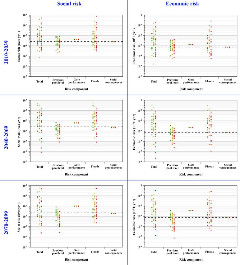
J. Fluixá-Sanmartín et al.: Quantification of climate change impact on dam failure risk                                           2121

Table 1. List of climatic projections (CP) used in the study, indicating the driving GCM, ensemble member, institute and RCM for each of
them, and which scenario is available.

 ID      Domain    Driving GCM                      Ensemble    Institute          RCM         Historical   RCP2.6   RCP4.5   RCP8.5
 CP1     EUR-11    CNRM-CERFACS-CNRM-CM5            r1i1p1      CLMcom         CCLM4-8-17          x                   x         x
 CP2     EUR-11    CNRM-CERFACS-CNRM-CM5            r1i1p1      SMHI              RCA4             x                   x         x
 CP3     EUR-11    ICHEC-EC-EARTH                   r12i1p1     CLMcom         CCLM4-8-17          x          x        x         x
 CP4     EUR-11    ICHEC-EC-EARTH                   r12i1p1     KNMI           RACMO22E            x          x        x         x
 CP5     EUR-11    ICHEC-EC-EARTH                   r12i1p1     SMHI              RCA4             x          x        x         x
 CP6     EUR-11    ICHEC-EC-EARTH                   r1i1p1      KNMI           RACMO22E            x                   x         x
 CP7     EUR-11    ICHEC-EC-EARTH                   r3i1p1      DMI             HIRHAM5            x          x        x         x
 CP8     EUR-11    IPSL-IPSL-CM5A-LR                r1i1p1      GERICS         REMO2015            x          x
 CP9     EUR-11    IPSL-IPSL-CM5A-MR                r1i1p1      IPSL-INERIS     WRF331F            x                   x         x
 CP10    EUR-11    IPSL-IPSL-CM5A-MR                r1i1p1      SMHI              RCA4             x                   x         x
 CP11    EUR-11    MOHC-HadGEM2-ES                  r1i1p1      CLMcom         CCLM4-8-17          x                   x         x
 CP12    EUR-11    MOHC-HadGEM2-ES                  r1i1p1      DMI             HIRHAM5            x                             x
 CP13    EUR-11    MOHC-HadGEM2-ES                  r1i1p1      KNMI           RACMO22E            x          x        x         x
 CP14    EUR-11    MOHC-HadGEM2-ES                  r1i1p1      SMHI              RCA4             x          x        x         x
 CP15    EUR-11    MPI-M-MPI-ESM-LR                 r1i1p1      CLMcom         CCLM4-8-17          x                   x         x
 CP16    EUR-11    MPI-M-MPI-ESM-LR                 r1i1p1      MPI-CSC        REMO2009            x          x        x         x
 CP17    EUR-11    MPI-M-MPI-ESM-LR                 r1i1p1      SMHI              RCA4             x          x        x         x
 CP18    EUR-11    MPI-M-MPI-ESM-LR                 r2i1p1      MPI-CSC        REMO2009            x          x        x         x
 CP19    EUR-11    NCC-NorESM1-M                    r1i1p1      DMI             HIRHAM5            x                   x         x
 CP20    EUR-11    NCC-NorESM1-M                    r1i1p1      SMHI              RCA4             x                             x
 CP21    EUR-11    NOAA-GFDL-GFDL-ESM2G             r1i1p1      GERICS         REMO2015            x          x

the dam failure (Serrano-Lombillo et al., 2011). The tree’s               The node failure modes contemplates the four possible
branches represent all the possible outcomes of their event of         ways in which the Santa Teresa dam is supposed to fail: due
origin and have an assigned probability. Any path between              to the overtopping of the dam or of the dike, or due to the
the initiating node and each of the nodes of the tree repre-           sliding of the dam or of the dike. For each branch the model
sents one of the possible outcomes that might result from the          relates the maximum water level reached in the reservoir in
original event and can be calculated as the product of the             each flood event with the conditional failure probability. It is
probabilities associated with each branch (Fluixá-Sanmartín            worth noting that the sliding failure mode is decomposed in
et al., 2019).                                                         two nodes: hypothesis of the probability of being in different
   This model can be represented using the influence diagram           uplift pressures (dam/dike uplift pressures) and the existing
presented in Fig. 3. As suggested in Fluixá-Sanmartín et al.           capacity to detect and to avoid high uplift pressures (no de-
(2018), this risk modelling approach is used in this work to           tection).
structure and organize the assessment of the potential im-                Finally, the following nodes are used to compute conse-
pacts of climate change on the different components of risk.           quences in order to estimate risk, following Eq. (1). The node
   In the first five nodes the model defines the probability           Q failure characterizes the failure hydrograph for each failure
of different dam–reservoir system scenarios prior to the ar-           mode by introducing a relation between the water pool level
rival of the largest flood of the year. This encompasses the           and the peak failure discharge. This relation was previously
probability of falling in a specific period of the year (sea-          computed using hydraulic models of the dam breach.
son), whether its daytime or night-time (day/night), the an-              The last nodes introduce the relation between the outflow
nual exceedance probability curve of the water pool level of           hydrographs and the economic (econ. conseq. (failure)) and
the reservoir (previous pool level) and the probability of the         loss of life consequences (social conseq. (failure)). A com-
bottom outlet works and spillway gates functioning properly            mon practice in dam safety is working with incremental con-
(or not) when a flood arrives (spillway av. and outlet av.). The       sequences, obtained by subtracting the consequences for the
next node (floods) introduces the flood entering the reservoir;        non-failure case from the consequences for the failure case
a probabilistic hydrologic analysis is necessary to obtain the         (Serrano-Lombillo et al., 2011; SPANCOLD, 2012; USACE,
annual exceedance probability of potential incoming floods.            2011) in order to consider only the part of the incremen-
The following node (flood routing) includes the maximum                tal risk produced by the dam failure. Therefore, the conse-
pool levels and peak outflows resulting from the flood routing         quences of the non-failure case (econ. conseq. (no failure)
for each possible combination of previous pool level, inflow           and social conseq. (failure)) must also be calculated to ob-
flood and gate availability.                                           tain incremental consequences.

www.nat-hazards-earth-syst-sci.net/19/2117/2019/                              Nat. Hazards Earth Syst. Sci., 19, 2117–2139, 2019
2122                                J. Fluixá-Sanmartín et al.: Quantification of climate change impact on dam failure risk

Figure 3. Diagram of the quantitative risk model for the Santa Teresa dam.

4.4    Water resource management model                                 Table 2. Seasonal minimum and maximum volumes (h m3 ) and wa-
                                                                       ter levels (m a.s.l.) for the Santa Teresa reservoir.
Risk modelling requires the analysis of the probability of
occurrence of a certain water level in the reservoir at the              Month        Minimum    Maximum     Minimum      Maximum
moment of arrival of the flood. It defines the starting situa-                         volume     volume       level        level
tion in the reservoir when studying the loads induced by the                           (h m3 )    (h m3 )    (m a.s.l.)   (m a.s.l.)
flood (SPANCOLD, 2012). Such analysis can be usually per-                January         80         396       861.26       881.31
formed by using the register of historic pool levels. However,           February        80         396       861.26       881.31
the effects of climate change are expected to affect the future          March           80         436       861.26       883.13
water availability mainly due to increased precipitation vari-           April           80         461       861.26       884.20
ability and potential evapotranspiration (IPCC, 2014). There-            May             80         496       861.26       885.70
fore, the simulation of the system of water resource manage-             June            80         496       861.26       885.70
ment under future conditions is necessary to obtain the rela-            July            80         496       861.26       885.70
tion between water pool level and probability of exceedance.             August          80         496       861.26       885.70
                                                                         September       80         496       861.26       885.70
   The simulation consists of a sequential calculation of the            October         80         496       861.26       885.70
allocation and use of the water resources based on the reser-            November        80         496       861.26       885.70
voir’s exploitation rules. Apart from the evaluation of the fu-          December        80         396       861.26       881.31
ture inflows of the system, this analysis requires as inputs
the basin management strategy and the water demand that
depends on the reservoir’s supply. Such information is con-               Another aspect considered is the limitation of water stor-
tained in the Hydrological Plan of the Duero River Basin               age in the Santa Teresa reservoir. Given the seasonality of
(Confederación Hidrográfica del Duero, 2015) that describes            high flows entering the reservoir, the hydrological plan con-
the exploitation rules of the 13 systems of the basin.                 siders freeboard volumes that vary throughout the year to
   In particular, the Tormes system is composed of the Santa           adapt to the expected incoming floods. The minimum and
Teresa and the Almendra reservoirs of 496 and 2649 h m3 of             maximum volumes and their corresponding water levels to
volume capacity respectively. The above-mentioned hydro-               be ensured each month in normal exploitation conditions are
logical plan describes the water demands according to their            detailed in Table 2. These limitations are important for es-
category: agricultural (7), fish farming (5), urban (1) and in-        timating water pool levels (Sect. 5.3.1). For this study, five
dustrial demands (1). The different demands of the Tormes              periods of the year have been established from these spec-
system are mainly satisfied using the Santa Teresa reservoir           ifications, coded as follows: Dec–Feb (December, January
according to the assignation rules established. It also spec-          and February), Mar (March), Apr (April), May–Nov (May,
ifies the minimum ecological discharges at different points            June, October and November), and summer (July, August
of the river that must be guaranteed through the reservoir’s           and September).
releases. Figure 4 shows a schematic diagram with the dis-
tribution to each water demand and its return to the system
according to the hydrological plan.

Nat. Hazards Earth Syst. Sci., 19, 2117–2139, 2019                               www.nat-hazards-earth-syst-sci.net/19/2117/2019/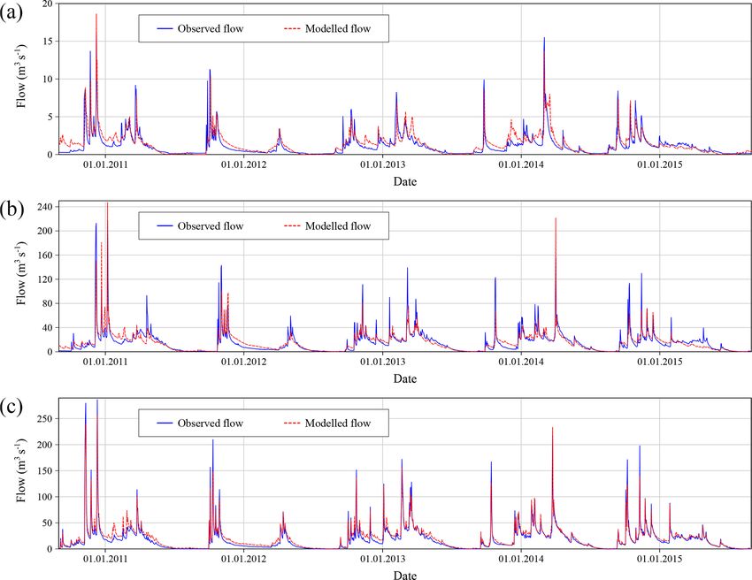
J. Fluixá-Sanmartín et al.: Quantification of climate change impact on dam failure risk                                     2123

                                                                     Once this transformation function has been defined, it is
                                                                  afterwards used to translate a simulated projection time series
                                                                  into a bias-corrected series. This procedure is applied sepa-
                                                                  rately for each climate projection (CP) described in Sect. 4.2
                                                                  (Table 1) and for each of the three future periods (1–3), using
                                                                  the historical period 1970–2005 as the calibration period of
                                                                  the correction function.
                                                                     Corrected values in between fitted transformed values have
                                                                  been approximated using a linear interpolation. When model
                                                                  values from climate projections are larger than the training
                                                                  values used to estimate the ECDF, the correction found for
                                                                  the highest quantile of the training period is used (Boé et al.,
                                                                  2007; Jakob Themeßl et al., 2011).
                                                                     In order to account for seasonally varying bias characteris-
                                                                  tics of the precipitation and temperature variables, the correc-
                                                                  tion function itself has been determined separately for each
                                                                  season. Moreover, when correcting the precipitation projec-
                                                                  tions, the number of wet days in the RCM time series of the
                                                                  historical period has also been adjusted to fit the number of
                                                                  wet days in the observed time series of the same period.
                                                                     Figure 5a shows an example of the empirical cumula-
                                                                  tive distribution functions (ECDFs) corresponding to the ob-
                                                                  served and the modelled CP3 historical time series of daily
                                                                  temperature, for the grid cell with coordinates 40◦ 050 6000 N,
                                                                  5◦ 480 0000 W. The required shift towards the right (increase)
Figure 4. Scheme of the main elements of the Tormes water re-     of the CP3 series for an ECDF of 0.4 to match the observa-
source system.                                                    tions has been highlighted with arrows. Figure 5b displays
                                                                  the bias-corrected temperatures (green line) from the orig-
5     Application of the methodology to the Santa Teresa          inal CP3 modelled time series (red line), compared to the
      dam                                                         observed series (blue line), for the year 1979.

5.1    Correction of the RCM projections                          5.2     Hydrological modelling

Each precipitation and temperature projection described in        5.2.1    Setting and calibration of the model
Sect. 4.2 has been bias-corrected using a statistical transfor-
mation. In particular, an empirical non-parametric quantile       A hydrological model of the Santa Teresa and the Tormes
mapping (eQM) approach (Boé et al., 2007; Panofsky and            catchments has been elaborated with the hydrological–
Brier, 1968) has been applied in this study using the R Soft-     hydraulic modelling software RS MINERVE (Foehn et al.,
ware (R Development Core Team, 2008). This method has             2019; García Hernández et al., 2019), a freeware that allows
been widely applied in climatology and more detailed infor-       rainfall–runoff calculations based on a semi-distributed con-
mation can be found in the extensive literature (Cannon et al.,   cept and downstream propagation of discharges.
2015; Gudmundsson et al., 2012; Gutjahr and Heinemann,               First, the basin has been divided into subbasins according
2013; Maraun, 2016).                                              to the hydrographic network and to the location of the gaug-
   The goal is to define the transformation function for a        ing stations, as shown in Fig. 2. For this study, the GSM-
modelled variable xmod so that its new distribution equals the    SOCONT model (Schaefli et al., 2005) has been applied to
distribution of the observed variable xobs corresponding to       each resulting subbasin. Simulated natural processes use pre-
the reference period, as defined in Eq. (2):                      cipitation and temperature inputs to model surface and sub-
        −1                                                        surface flow, infiltration, evapotranspiration, snow accumu-
xobs = Fobs (Fmod (xmod )) ,                               (2)
                                                                  lation and melting. Channel routing of the rivers has been
where Fmod is the empirical cumulative distribution func-         solved with the kinematic wave model, also available in
                               −1
tions (ECDFs) of xmod and Fobs     is the inverse ECDF (also      RS MINERVE.
named quantile function) corresponding to xobs . In this case,       Finally, the model’s calibration has been performed using
the RCM-derived daily outputs represent the modelled vari-        the calibration module of the RS MINERVE software based
ables while the daily data issued from the Spain02 v5 corre-      on the observed records of the gauging stations described in
spond to the observed variable.                                   Sect. 4.1. Calibrated parameters are the reference degree-day

www.nat-hazards-earth-syst-sci.net/19/2117/2019/                           Nat. Hazards Earth Syst. Sci., 19, 2117–2139, 2019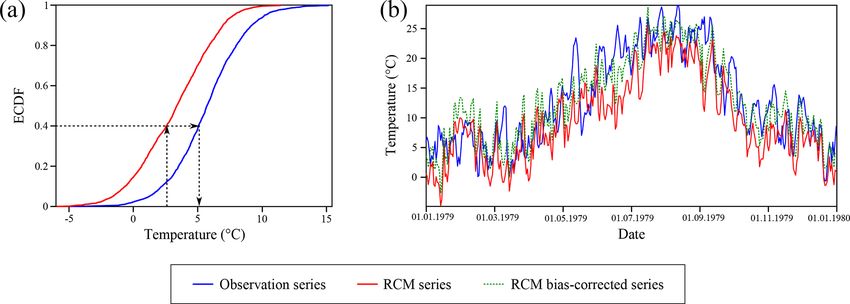
2124                                J. Fluixá-Sanmartín et al.: Quantification of climate change impact on dam failure risk

Figure 5. (a) Example of ECDF of the observed (blue) and the modelled CP3 (red) daily temperature series and bias correction using
the eQM technique: the ECDF of the simulated series (red) is shifted to match with the observed ECDF (blue). (b) Time series of daily
temperatures for the observed (blue) and the CP3 modelled (red) datasets and bias-corrected series (green, doted line) for the year 1979.

snowmelt coefficient (S), the maximum height of the infil-             Sect. 5.3.4. For that, the individual consumption has been
tration reservoir (HGR3Max), the release coefficient of the            maintained and only the number of consumers has been
infiltration reservoir (KGR3), and the runoff slope (J0 ) and          adapted. In the absence of more detailed information, the rest
Strickler coefficient (Kr ) for the runoff surface as well as          of the demands (agricultural, industrial and fish farming) and
for the river reaches. The performance indicators used to as-          the prioritization of the water supply for each demand (the
sess the quality of the fit are the Nash–Sutcliffe (Nash and           importance and order in which each demand is satisfied) are
Sutcliffe, 1970) and Kling–Gupta efficiencies (Gupta et al.,           assumed unaltered in future scenarios.
2009; Kling et al., 2012).                                                Concerning basin discharges, the hydrological model elab-
   Periods with available discharge data are heterogeneous             orated with RS MINERVE is able to simulate the rainfall–
and thus calibration/validation processes have been adapted            runoff processes at a daily resolution. Thus, the meteorologi-
accordingly. It has been decided to use the period 1 Octo-             cal data issued from the Spain02 grid observations as well as
ber 2010–30 September 2015 as the calibration period, while            from the climate projections are used as inputs to the model
the validation period depends on each gauging station. Re-             in order to obtain the consequent discharges at each subbasin
sults of the calibration/validation process for the gauging sta-       (Fig. 2).
tions upstream of the Santa Teresa dam (Hoyos del Espino,                 The simulation of the reservoir’s response has been mod-
Barco de Ávila and Puente Congosto) are presented in Ta-               elled including on the hydrological model different hydraulic
ble 3. Figure 6 shows the observed and modelled flows for              elements available in RS MINERVE. On the one hand, the
these stations. For visualization purposes, only the period            water consumption has been modelled with consumer ob-
1 October 2010–30 September 2015 is displayed. We con-                 jects which allow us to define the flow abstraction series
sider the calibration to present adequate results for the pur-         of each water demand (including the minimum ecological
pose of the study.                                                     discharges) at each time step. The order of preference de-
                                                                       fined in the hydrological plan guidelines for the supply to
5.2.2   Water management model simulation                              each demand has been respected. On the other hand, the out-
                                                                       flows from the reservoir are managed using planner objects:
                                                                       these models permit us to create different rules that rest on
The first purpose of the hydrological model of the Santa
                                                                       the hydrological and hydraulic conditions of the basin. That
Teresa and Tormes catchments is the simulation of the wa-
                                                                       is, the supply to a specific point depends on the demand at
ter resources and its evolution with time. The basic inputs re-
                                                                       this point, the water level at the reservoir or the satisfaction
quired are (i) the reservoir’s exploitation rules, (ii) the water
                                                                       of preferential demands. At this point, it is worth mention-
demands and (iii) the expected discharges at different points
                                                                       ing that the seasonal minimum and maximum levels contem-
of the basin.
                                                                       plated by the hydrological plan (Table 2) have been incor-
   The first two inputs are extracted from the Hydrological
                                                                       porated to the model within these planner objects. More de-
Plan of the Duero River Basin (Confederación Hidrográfica
                                                                       tailed descriptions on the use of such models can be found in
del Duero, 2015) described in Sect. 4.3. For this study, the
                                                                       García Hernández et al. (2019).
only demand that is considered variable with time is the ur-
                                                                          The validation of this water resource model is conducted
ban demand, which corresponds to the supply to the city of
                                                                       by comparing its results with a reference record. Figure 7 dis-
Salamanca. This is a direct consequence of the population
                                                                       plays the observed water levels recorded at the Santa Teresa
variation expected at this city, which is further described in

Nat. Hazards Earth Syst. Sci., 19, 2117–2139, 2019                             www.nat-hazards-earth-syst-sci.net/19/2117/2019/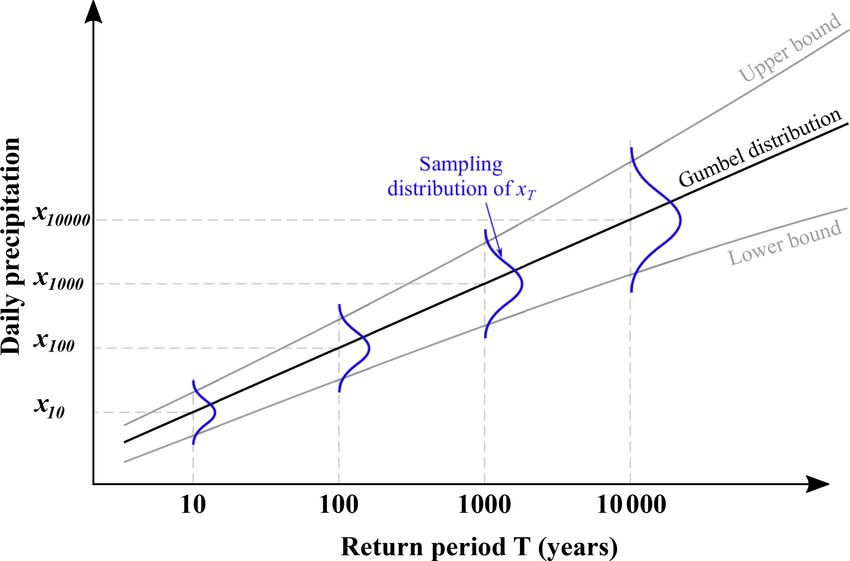
J. Fluixá-Sanmartín et al.: Quantification of climate change impact on dam failure risk 2125
Table 3. Calibration and validation results for the gauging stations upstream of the Santa Teresa dam.
Station Calibration Validation
Period Nash Kling–Gupta Period Nash Kling–Gupta
Hoyos del Espino 1 Oct 2010–30 Sep 2015 0.612 0.749 1 Oct 1983–1 Oct 1995 0.570 0.726
Barco de Ávila 1 Oct 2010–30 Sep 2015 0.679 0.766 1 Oct 1971–30 Sep 1987 0.667 0.589
Puente Congosto 1 Oct 2010–30 Sep 2015 0.939 0.768 1 Oct 1997–30 Sep 2010 0.670 0.709
Figure 6. Comparison between observed (blue) and modelled (red) flows for the gauging stations (a) Hoyos del Espino, (b) Barco de Ávila
and (c) Puente Congosto.
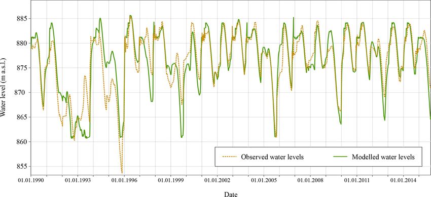
reservoir and the simulated series obtained with the RS MIN- considered that the overall performance of the hydrological
ERVE model, for the period 1990–2015. As shown in the fig- model is adequate to simulate the water resources at the Santa
ure, result performance is moderate at the beginning of the Teresa reservoir. Once the model is validated, the different
period (1990–2000) and then increases notably from 2000 simulations have been processed for the historical and the
to 2015. This is mainly due to the fact that the reservoir’s future periods.
exploitation rules used in the model are based on the last
hydrological plan of the basin (Confederación Hidrográfica 5.2.3 Design flood hydrographs
del Duero, 2015), which is relatively recent. It is likely that
before 2000 the operational rules were different and thus Additionally, the hydrological model has been employed for
the model is not capable of capturing the real fluctuations the definition of the design flood hydrographs entering the
of the water resources. For the purposes of the study, it is Santa Teresa reservoir. A deterministic approach based on
the design storm method (ASCE, 1996; Reed et al., 1999)
www.nat-hazards-earth-syst-sci.net/19/2117/2019/ Nat. Hazards Earth Syst. Sci., 19, 2117–2139, 2019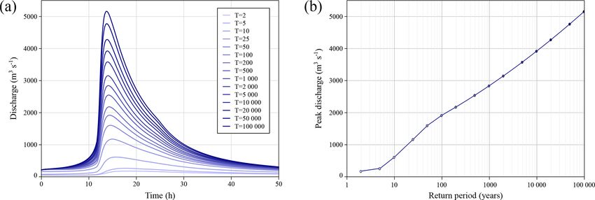
2126                                J. Fluixá-Sanmartín et al.: Quantification of climate change impact on dam failure risk

Figure 7. Observed and simulated water levels at the Santa Teresa reservoir, between 1990 and 2015.

has been followed. In this method, a design storm is defined
based on the intensity duration frequency (IDF) curve of rain-                         280.1 −t 0.1
                                                                       It         I1       280.1 −1
fall and applied to an event-based hydrological model to cal-             =                             ,                          (3)
                                                                       Id         Id
culate the hydrographs. Statistical methods have been dis-
carded mainly due to a lack of representative flood records, in        where It is the average intensity (mm h−1 ) corresponding to
particular for the characterization of future floods. The pro-         the time interval of duration t; Id is the daily average inten-
cess consists of three main parts: the generation of synthetic         sity (mm h−1 ) corresponding to the return period considered,
storms, the definition of the initial conditions of the basin          and equal to Pd /24; Pd is the total daily precipitation (mm)
and the simulation of the flood hydrographs. What follows is           corresponding to the return period considered; I1 /Id is the
a detailed description of these steps. It is worth mentioning          ratio between the hourly and daily intensity, obtained from
that the process has been individually applied to the differ-          Ministerio de Fomento (2016) and equal to 10.2 for the study
ent periods considered (historical, 1–3) in order to assess the        case.
changes in the resulting floods from the base case until the              It is worth mentioning that this formula is climate- and
end of the 21st century.                                               location-dependent since it has been extracted from an anal-
                                                                       ysis based on historical records. However, in this study the
Generation of design storm hyetographs                                 formula has also been applied for future climatic conditions.
                                                                       The difficulty to establish IDF relations with no sub-daily
The definition of the design storm hyetograph first requires           precipitation data available is one of the limitations of the
the statistical analysis of the annual maxima of storm rainfall,       present work. Thus, in order to deal with this issue, the op-
extracted from the daily precipitation data of the observation         tion chosen was to rely on predefined formulations such as
and climate projection series for each point of the Spain02            the one presented in Eq. (3).
grid. This allows us to obtain the maximum daily precipita-               Temporal rainfall distribution is obtained using the alter-
tion for any return period considered. Each annual maxima              nating block method (Chow et al., 2008), where the inten-
series has been fitted to a Gumbel distribution, a widely used         sity of each time interval is read from the previous IDF
option in the Spanish territory. Once the distribution fitted,         curve. Subsequently, the rainfall depths for each interval (P1,
the daily precipitations corresponding to the following re-            P2, . . . ) are obtained taking the difference between succes-
turn periods were calculated: 2, 5, 10, 25, 50, 100, 200, 500,         sive rainfall depth values, with 1t = 0.5 h. The blocks P1,
1000, 2000, 5000, 10 000, 20 000, 50 000 and 100 000 years.            P2, . . . are reordered with the maximum intensity at the cen-
In order to evaluate the sensitivity of risk results to the fitted     tre of the hyetograph and the other blocks alternating to the
Gumbel distribution, a complementary sensitivity analysis is           right and left. In the absence of more detailed information, a
included in Appendix A.                                                storm event duration of 24 h has been used.
   Then, a predefined IDF curve has been used to estimate the             Given that rainfall is never evenly distributed over the area
rainfall depth for any given duration and for the selected re-         of study due to the topographic variability of the catchment
turn periods. The formulation of the IDF curve is taken from           areas, the use of an areal reduction factor (ARF) is required
the document of Ministerio de Fomento (2016) and is ex-                to correct each grid point rainfall and avoid an overestimation
pressed as                                                             of the rainfall input. The ARF adopted follows the empirical

Nat. Hazards Earth Syst. Sci., 19, 2117–2139, 2019                                www.nat-hazards-earth-syst-sci.net/19/2117/2019/
J. Fluixá-Sanmartín et al.: Quantification of climate change impact on dam failure risk 2127
formulation proposed in Témez (1991) for the Spanish terri-
tory:
log(A)
ARF = 1 − , (4)
15
where A is the area of the catchment (km2 ). In this case, the
drainage area of the Santa Teresa reservoir is 1853 km2 .
Initial basin conditions
Francés et al. (2012) and Rogger et al. (2012) highlighted an
important drawback when applying the design storm method.
It is generally assumed that the rainfall and the discharge
return periods are equal, and no other factors such as the Figure 8. Example of ECDF curve for the soil saturation (relative
initial conditions of the basin are generally considered. In- HGR3 state variable) and extraction of the value corresponding to a
deed, the proper selection of basin antecedent conditions is non-exceedance probability of 0.9.
of paramount importance for the runoff definition.
To address such limitation, an analysis of three different
state variables of the hydrological model was performed: 5.3 Risk modelling
the level in the infiltration reservoir (HGR3), the runoff wa-
ter level downstream of the surface (Hr ) and the river dis- Considering the exposure of the dam to climate change, the
charge (Q). The goal was to define a characteristic initial risk model of the Santa Teresa dam (Fig. 3) is updated fol-
state of the basin prior to the occurrence of each storm. lowing the effects of climate change on each of the risk com-
Once the hydrological model was set, it was used to run ponents. Among these components, mainly four have been
the rainfall–runoff simulations corresponding to the differ- identified as susceptible to being altered: previous pool levels
ent scenarios (observations and projections) and for all the in the reservoir, spillway gate and bottom outlet performance,
periods considered (historical, period 1–period 3). For each floods entering the reservoir, and social consequences used to
simulation, the dates on which the annual maximum rain- compute the social risk. In the absence of more detailed anal-
falls occurred were identified, allowing us to extract the state yses, in this study other risk model components are assumed
variables of the model corresponding to the precedent day. unaltered.
This resulted in a set of state variables per year for each
5.3.1 Previous pool level
simulation. From each of these series of state variables, an
ECDF curve was generated. In this way, the initial condi- Based on the reservoir levels obtained from the water re-
tions matching with the storm hyetograph of return period T sources simulation of each scenario defined in Sect. 5.2.2,
can be obtained by reading from the ECDF curve the value the empiric exceedance probability curve of the pool levels is
for a non-exceedance probability equal to 1 − 1/T . Figure 8 obtained by ordering all the data in increasing order (SPAN-
illustrates the extraction of the soil saturation (calculated COLD, 2012) and applying Eq. (5):
as HGR3/HGR3Max × 100 for the SOCONT model) corre-
sponding to a non-exceedance probability of 0.9 or a return in − 1
period of 10 years. PEn = 1 − , (5)
N −1
Hydrograph calculation where PEn is the probability of exceedance for a pool level n,
in is the number of order of pool level n within the series of
The model developed with RS MINERVE and described sorted levels and N is the length of the series.
above was used as the event-based hydrological model to The resulting curve is discretized in different not equidis-
simulate the behaviour of the Santa Teresa basin. In this case, tant intervals to be included within the risk model event tree.
the simulation time step was set at 10 min in order to bet- In the event tree, the probability of each branch is the proba-
ter capture the hydrological processes occurring in the basin. bility of falling within any of the values of the interval con-
Once each storm hyetograph and set of initial conditions cor- sidering a representative value of each interval – usually the
responding to a return period between 2 and 100 000 years average value of the interval. Since the risk model used in
has been defined, the model is run, and the flood hydrographs this study considers the specific period of the year in which
are obtained. the flood occurs, the reservoir’s exploitation rules differ de-
Resulting floods for the base case are presented in Fig. 9a. pending on this period (Sect. 4.3) and thus imply different
Peak discharge by return period is displayed in Fig. 9b. exceedance probability curves of the pool levels. The anal-
ysis of the previous pool level must therefore be carried out
www.nat-hazards-earth-syst-sci.net/19/2117/2019/ Nat. Hazards Earth Syst. Sci., 19, 2117–2139, 20192128 J. Fluixá-Sanmartín et al.: Quantification of climate change impact on dam failure risk
Figure 9. (a) Resulting flood hydrographs for return periods between 2 and 100 000 years, for the base case. (b) Flood frequency characteri-
zation of the maximum values of peak discharges.
– 95 %. The outlet is new or has been very well main-
tained.
– 85 %. The outlet is well maintained but has had some
minor problems.
– 75 %. The outlet has some problems.
– 50 %. The outlet is unreliable for flood routing.
– 0 %. The outlet is not reliable at all or it has never been
used.
Figure 10. Relation between water pool level and probability of ex- In this analysis, gates can be considered independent and
ceedance for the base case (present situation) and the climate pro- thus the probability of each availability gate case can be esti-
jection CP1 (RCP45 and period 1), for the summer season. mated with a binomial distribution (Eq. (6)):
n!
P (x) = · p x · (1 − p)n−x , (6)
for each of the periods considered. Figure 10 shows the com- x! · (n − x)!
parison of the exceedance probability curves corresponding
where P (x) is the probability that x number of gates work
to the base case and to the climate scenario CP1 (RCP45 and
properly, n is the total number of gates and p is the individual
period 1), both computed for the summer season. As can be
reliability of gates.
seen, the results of the CP1 projection present lower water
As part of the quantitative risk analysis performed on the
levels than for the base case. This is mainly due to the reduc-
Santa Teresa dam, the state of the spillway gates and the bot-
tion in the discharge contributions to the reservoir and the
tom outlet was estimated as well maintained. Their individ-
enhanced evapotranspiration directly related to the increase
ual reliabilities were thus established as 85 % for the present
in temperatures.
situation. However, the conditions of the gates can deterio-
5.3.2 Gate performance rate with time and with changing hydro-meteorological con-
ditions. As mentioned in Fluixá-Sanmartín et al. (2018), cer-
In the context of dam safety, spillways and outlet works play tain factors such as increased soil erosion due to more in-
a fundamental role. The estimation of their reliability, i.e. that tense rainfalls or greater fluctuations in temperature could
in the moment of the arrival of the flood they can be used, eventually lead to a decreased reliability of the gates. In this
makes part of the studies required to feed a risk model. In a study, the state of both the spillway and the bottom outlet
basic analysis, individual reliability can be estimated directly gates is assumed to progressively deteriorate until the end of
for each gate using the qualitative description of the gate sys- the 21st century. Following a simple approach, it is consid-
tem’s condition. Escuder-Bueno and González-Pérez (2014) ered that some problems may appear and thus the individ-
propose a classification based on these descriptors that avoids ual reliability will vary from 85 % to 75 %, corresponding to
resorting to detailed studies such as fault trees. period 3 (2070–2099). For the intermediate scenarios a lin-
ear interpolation is applied to obtain the individual reliability,
Nat. Hazards Earth Syst. Sci., 19, 2117–2139, 2019 www.nat-hazards-earth-syst-sci.net/19/2117/2019/J. Fluixá-Sanmartín et al.: Quantification of climate change impact on dam failure risk 2129
that is 81.5 % for period 1 (2010–2039) and 78.5 % for pe- order to work only with present values, independently of the
riod 2 (2040–2069). future scenario considered.
5.3.3 Floods
6 Results and discussion
Since the present study analyses the risk of the dam under
a hydrological scenario, it is supposed that the floods are Once the dam risk model is adapted following the effects of
the main loads to which the dam is subjected. Therefore, climate change on each of the risk components, the social
the resulting flood hydrographs obtained in Sect. 5.2.3 have and economic risks (consequences per year) are calculated
been incorporated to update the risk model of the dam. As for the base case and for all the CP–period–RCP combina-
described above, each hydrograph is characterized by its re- tions. For the base case (present situation), the failure proba-
turn period or annual exceedance probability, which defines bility is 2.91 × 10⁻⁶ per year, while the social and economic
the probability associated with each branch of the risk model risks are 2.56×10⁻⁴ lives per year and EUR 7.53×10⁻⁴ mil-
emerging from the floods node (Fig. 3). This also has an im- lion per year respectively.
pact on the outcomes of the dam’s flood routing, in particular The evolution of social and economic risks for each RCP,
the maximum pool levels and the peak outflows. It has been from the present situation until the end of the 21st century, is
considered, however, that the flood routing strategy remains presented in Fig. 11. For illustrative purposes, the y axis is
unchanged as defined in the operation rules document of the plotted on a logarithmic scale to better appreciate the order
dam. of magnitude of its values. The dashed black line indicates
the present risk and helps highlight whether the future risk of
5.3.4 Social consequences a particular CP is above or under such reference risk level.
In general, these results indicate that in most future scenarios
The dam risk model used in this study considers the social a deterioration of both the social and economic risks occurs.
consequences resulting from the dam failure (Fig. 3), which Indeed, the risk tends to increase in comparison to the present
rely on the exposure of people in the at-risk area to the dam risk level and a certain dispersion of the risk appears with
output hydrograph. These consequences correspond to the time. However, the RCP8.5 cases present a wider dispersion
number of fatalities among the inhabitants of the different of results and no homogeneous effects can be extracted from
population nuclei between the Santa Teresa and the Almen- it.
dra dams. In order to deepen in the analysis, the resulting risks have
Under future scenarios, the evolution of population at risk been decomposed in their associated probability of failure
is thus expected to affect the potential casualties and needs to and average consequences. Figure 12 represents this disag-
be considered to adequately assess the social risk. This does gregation of social and economic risks for each period con-
not account for a direct effect of climate change; however, sidered. In such a graph, risk is the dimension that combines
this non-climatic factor has been considered in this study in both axes and is smaller in the lower left corner and grows
order to contemplate a more realistic situation in future sce- towards the upper right corner. This is a widely used type of
narios. representation, used for instance by the US Bureau of Recla-
For this analysis, the long-term population projections at mation (USBR, 2011) to propose tolerability recommenda-
national scale available in the online publication Our World tions for incremental risk. Logarithmic scales are used in
in Data (2018) extracted from the UN database (United Na- both axes and the same legend as in Fig. 11 is applied for
tions, 2017) were used. According to these projections, pop- the points. The present risk level has been represented as a
ulation is expected to slightly decrease until 2040 and will black point and its probability of failure and consequences
follow a substantial diminution until the end of the century. are highlighted with two dashed black lines. These lines di-
It has been supposed that the same pattern at the national vide the graph in four quarters labelled as
level can be replicated at the regional and local levels. There-
– Type I, cases where the failure probability is greater, and
fore, in order to adapt the dam risk model used, the popu-
the consequences are lower than in the base case.
lation at risk in the different cities and settlements has been
proportionally reduced under the three future scenarios en- – Type II, cases where both the failure probability and the
visaged. Hence, the relative variation compared to the pop- consequences are greater than in the base case.
ulation in 2010 is as follows: −2.52 % for period 1 (2010–
2039), −14.37 % for period 2 (2040–2069) and −22.25 % – Type III, cases where both the failure probability and
for period 3 (2070–2099). the consequences are lower than in the base case.
It is worth mentioning that, for the assessment of the eco-
nomic consequences, the same current assets and services at – Type IV, cases where the failure probability is lower,
risk remain so in the future and no new services are consid- and the consequences are greater than in the base case.
ered. Moreover, their economic cost has not been updated in
www.nat-hazards-earth-syst-sci.net/19/2117/2019/ Nat. Hazards Earth Syst. Sci., 19, 2117–2139, 20192130 J. Fluixá-Sanmartín et al.: Quantification of climate change impact on dam failure risk Figure 11. Social and economic risk results (a–f), classified by RCP. The base case (BC) situation is highlighted with a black point and a dashed line. Moreover, Tables 4 and 5 present the percent of cases Since in this study the different components of the falling in each of these situations, grouped by period and risk model have been adapted and analysed concurrently RCP. These results exhibit a tendency of the cases analysed (Sect. 5.3), risk results do not highlight the individual contri- to be in the Type I situation, and a lower proportion in the bution of each component to the final risk state. However, the Type III situation, for all the periods analysed. Therefore, use of risk models allows us to decompose the contribution most cases indicate a reduction in the average consequences of each node in the final risk. For this purpose, a sensitivity (not only due to the diminished exposure of people in the at- analysis has been performed on the different risk components risk area) as well as an increase in the probability of failure (previous pool level, gate performance, floods and social con- of the dam. sequences) and their effect on the final dam failure risk, com- Nat. Hazards Earth Syst. Sci., 19, 2117–2139, 2019 www.nat-hazards-earth-syst-sci.net/19/2117/2019/
You can also read