European Journal of Agronomy
←
→
Page content transcription
If your browser does not render page correctly, please read the page content below
European Journal of Agronomy 128 (2021) 126306
Contents lists available at ScienceDirect
European Journal of Agronomy
journal homepage: www.elsevier.com/locate/eja
Dynamic simulation of management events for assessing impacts of climate
change on pre-alpine grassland productivity
Krischan Petersen a, David Kraus a, Pierluigi Calanca b, Mikhail A. Semenov c,
Klaus Butterbach-Bahl a, Ralf Kiese a, *
a
Institute for Meteorology and Climate Research, Karlsruhe Institute of Technology, Kreuzeckbahnstraße 19, 82467, Garmisch-Partenkirchen, Germany
b
Agroscope Institute for Sustainability Sciences ISS, Reckenholzstrasse 191, P.O. Box 8046, Zürich, Switzerland
c
Rothamsted Research, Harpenden, Hertfordshire, AL5 2JQ, UK
A R T I C L E I N F O A B S T R A C T
Keywords: The productivity of permanent temperate cut grasslands is mainly driven by weather, soil characteristics,
Mountainous grasslands botanical composition and management. To adapt management to climate change, adjusting the cutting dates to
Biomass yields reflect earlier onset of growth and expansion of the vegetation period is particularly important. Simulations of
Process-based modelling
cut grassland productivity under climate change scenarios demands management settings to be dynamically
Growing season
derived from actual plant development rather than using static values derived from current management op
Adaptive management
erations. This is even more important in the alpine region, where the predicted temperature increase is twice as
high as compared to the global or Northern Hemispheric average.
For this purpose, we developed a dynamic management module that provides timing of cutting and manuring
events when running the biogeochemical model LandscapeDNDC. We derived the dynamic management rules
from long-term harvest measurements and monitoring data collected at pre-alpine grassland sites located in S-
Germany and belonging to the TERENO monitoring network. We applied the management module for simula
tions of two grassland sites covering the period 2011–2100 and driven by scenarios that reflect the two repre
sentative concentration pathways (RCP) 4.5 and 8.5 and evaluated yield developments of different management
regimes.
The management module was able to represent timing of current management operations in high agreement
with several years of field observations (r2 > 0.88). Even more, the shift of the first cutting dates scaled to a +1 ◦ C
temperature increase simulated with the climate change scenarios (− 9.1 to − 17.1 days) compared well to the
shift recorded by the German Weather Service (DWD) in the study area from 1991− 2016 (− 9.4 to − 14.0 days).
In total, the shift in cutting dates and expansion of the growing season resulted in 1− 2 additional cuts per year
until 2100. Thereby, climate change increased yields of up to 6 % and 15 % in the RCP 4.5 and 8.5 scenarios with
highest increases mainly found for dynamically adapted grassland management going along with increasing
fertilization rates. In contrast, no or only minor yield increases were associated with simulations restricted to
fertilization rates of 170 kg N ha− 1 yr− 1 as required by national legislations. Our study also shows that yields
significantly decreased in drought years, when soil moisture is limiting plant growth but due to comparable high
precipitation and water holding capacity of soils, this was observed mainly in the RCP 8.5 scenario in the last
decades of the century.
1. Introduction 2018). In addition to the economic relevance of fodder production for
dairy and cattle farming (Sándor et al., 2017), grasslands fulfill a
Permanent grassland cover almost one third of the agricultural land number of other key ecosystem services like water retention, biodiver
area in Germany and is the dominant land use in the alpine and pre- sity, erosion control and soil fertility (Bengtsson et al., 2019; Gibson,
alpine region of S-Germany (Dierschke and Briemle, 2002; Kiese et al., 2009). Beside diverse effects of climate change on these ecosystem
* Corresponding author.
E-mail addresses: krischan.petersen@kit.edu (K. Petersen), david.kraus@kit.edu (D. Kraus), pierluigi.calanca@agroscope.admin.ch (P. Calanca), mikhail.
semenov@rothamsted.ac.uk (M.A. Semenov), klaus.butterbach-bahl@kit.edu (K. Butterbach-Bahl), ralf.kiese@kit.edu (R. Kiese).
https://doi.org/10.1016/j.eja.2021.126306
Received 8 October 2020; Received in revised form 28 April 2021; Accepted 3 May 2021
1161-0301/© 2021 The Author(s). Published by Elsevier B.V. This is an open access article under the CC BY license (http://creativecommons.org/licenses/by/4.0/).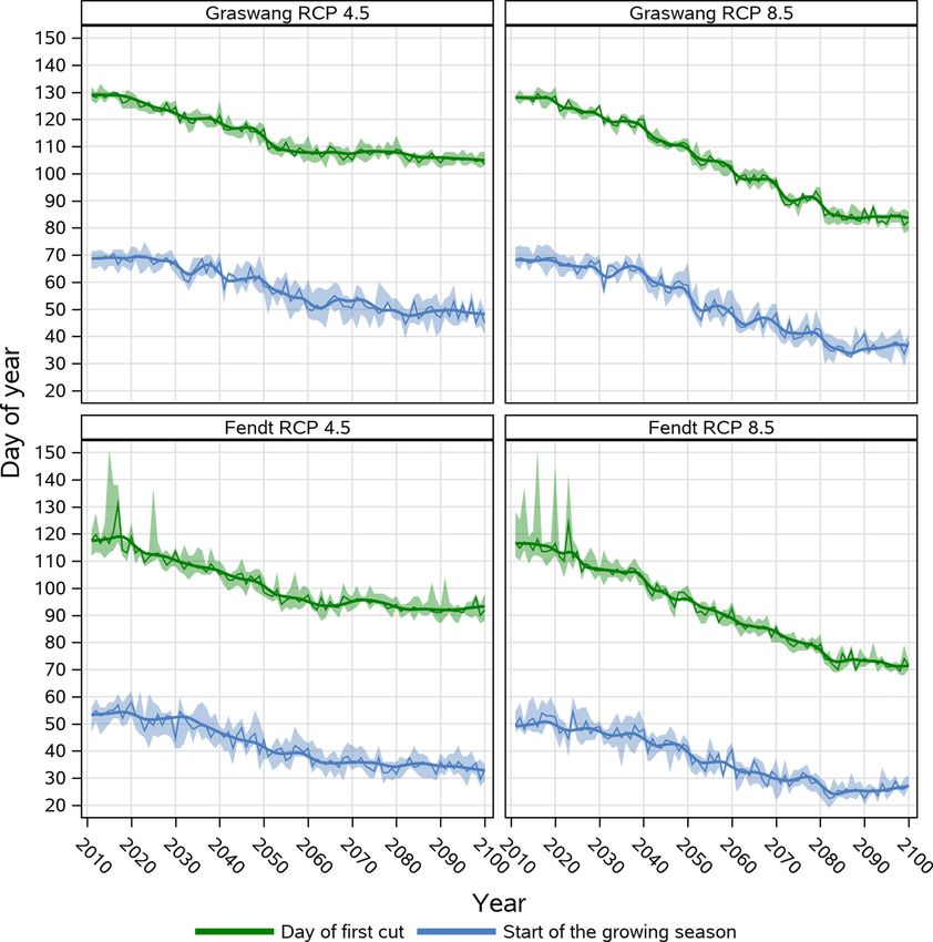
K. Petersen et al. European Journal of Agronomy 128 (2021) 126306
functions (Hopkins and Del Prado, 2007; Lee et al., 2013; Soussana et al., by applying thresholds for accumulated GDD for the first and following
2013; Wang et al., 2016; Wiesmeier et al., 2013), productivity is ex cuts (Höglind et al., 2013; Jing et al., 2014, 2013; Thivierge et al., 2016).
pected to increase in temperate and cold grasslands (Wang et al., 2019) Results from these studies underline the importance of accounting for
as far as water availability is not limiting (Dellar et al., 2018; Soussana additional cutting events (Höglind et al., 2013; Jing et al., 2014) with up
et al., 2013). This effect needs to be examined particularly in the to 10 % increase in annual yields using adapted instead of static man
pre-alpine and alpine regions where average warming is predicted to be agement for grassland sites in Canada (Thivierge et al., 2016). However,
at a pace twice as high as compared to the global or Northern Hemi not taking into account limitation of plant growth under drought con
spheric average (Auer et al., 2007) and will likely accelerate in coming ditions or stimulation of plant growth by increasing atmospheric CO2
decades (Gobiet et al., 2014; Smiatek et al., 2016). The stimulating effect concentration can be a disadvantage of only temperature informed GDD
on plant biomass production caused by increasing temperatures and based grassland modelling approaches.
higher atmospheric CO2 concentrations influences future cutting and Therefore, we present in this study a new dynamic management
fertilization regimes (Chang et al., 2017; Soussana and Lüscher, 2007). approach that we implemented in the biogeochemical model Land
According to local agricultural practice, farmers cut the grass regularly scapeDNDC (Haas et al., 2013; Kraus et al., 2015), which dynamically
based on yield demands and maturity stage as influenced by weather provides timing of grassland management under varying climatic con
and soil conditions (Deroche et al., 2020), thus significant changes in ditions. We developed management rules based on long-term compre
biomass development will likely change the timing of cutting and hensive field measurements of grassland biomass and records of local
associated fertilization events throughout the year (Thivierge et al., farmers’ management decisions regarding cutting and manuring events
2016). Recent climate change has been found to affect species’ from grassland sites belonging to the TERENO preAlpine observatory
phenology in mid- and higher latitudes, especially regarding the earlier (Kiese et al., 2018). With this tool we automatically calculated execution
onset of spring events with mean global average changes of 2.3 days per of cuts based on simulated weather depending plant development and
decade (Parmesan and Yohe, 2003). Menzel et al. (2020) recently re tested the predicted timing and frequency of events with independent
ported an increase of the growing season of +0.261 ± 0.008 days per field data and phenological observations provided by the German
year and a shortening of the farming season of cropland by Weather Service (DWD). Finally, we ran simulations of grassland
− 0.149 ± 0.022 days per year in the period 1951–2018 using European biomass production spanning 2011− 2100 under climate change con
plant phenology data. ditions that reflect the Representative Concentration Pathways (RCP)
Modelling studies can help to assess the influence of different man 4.5 and 8.5, and evaluated differences in yields with dynamic and fixed
agement practices, agricultural adaptions (Gómara et al., 2020; Sándor schedules of management events. To further explore potentials of the
et al., 2018) and future climate changes on the above mentioned key dynamically adapted management under climate change conditions we
grassland functions by executing long-term climate change scenario conducted simulations with common nitrogen fertilization rates
simulations (Chang et al., 2017; De Bruijn et al., 2012; Graux et al., (200− 240 kg N ha− 1 yr− 1) and a scenario with reduced rates (≤ 170 kg
2013; Höglind et al., 2013; Kipling et al., 2016; Owen et al., 2015). The N ha− 1 yr− 1) following adoptions of the German fertilizer ordinance in
response of grassland productivity and functional diversity to climate 2018. Our hypothesis is that pre-alpine grassland simulations with static
change is complex as it implies interactions of weather with soil water management can lead to significantly lower yields than dynamic man
and nutrient availability as well as execution of management routines. agement simulations, and that reduced rates of N fertilization will result
Fixed annual schedules of management actions derived from current in lower yields particularly under climate change conditions.
climatic conditions are inappropriate for simulating future grassland
productivity under changing climate conditions and are likely to cause 2. Material and methods
bias in simulated grassland productivity. However, due to dynamic
changes between years the setup and timing of management events is 2.1. Study region and field site description
highly complex and thus was identified as one of the main challenges for
model based climate impact studies of grassland ecosystems (Kipling The new dynamic management module implemented into Land
et al., 2016). scapeDNDC (see Section 2.3) was developed, calibrated and tested with
So far, many modelling studies on cut grasslands simulated climate long-term field measurements of biomass harvest and respective man
change scenarios without an adaption of management (e.g. Abalos et al., agement data of two grassland sites, i.e. Graswang and Fendt (Ger
2016; Cordeiro et al., 2019; De Bruijn et al., 2012; Graux et al., 2013; many), located in the TERENO preAlpine Observatory (Kiese et al.,
Lazzarotto et al., 2010; Yang et al., 2018). An automatic management 2018) which covers parts of the Bavarian Alps (Ammergau Mountains)
routine was first widely used for regional simulations by Vuichard et al. and their foothills.
(2007), who integrated dynamic decision rules into the PaSIM model The high elevation site Graswang (47◦ 34’ 12.936” N lat., 11◦ 1’
(Riedo et al., 1998, 2000). This algorithm determines cutting dates by 54.804” E lon.) is situated in an alpine valley at 864 m.a.s.l. and is
maximizing the seasonal dry matter production. It triggers a cut after a characterized by a mean annual temperature (MAT) of 6.9 ◦ C and a
minimum of 30 days of regrowth and declining plant growth rates mean annual precipitation (MAP) of 1347 mm. The low elevation site
during 10 consecutive days. This approach was adopted for regional Fendt (47◦ 49’ 56.748” N lat., 11◦ 3’ 39.996” E lon.) is situated in the
simulations by Chang et al. (2015), single site simulations by Gómara foothills of the Alps at 595 m.a.s.l. with 8.9 ◦ C MAT and 956 mm MAP
et al. (2020) and even for regional climate change assessments (Chang (Table 1). The soil at Graswang is fluvic calceric Cambisol characterized
et al., 2017). Another relatively simplistic mechanism for regional by high clay as well as organic C (6.4 %) and total N (0.7 %) contents. In
simulations was developed by Rolinski et al. (2018) with the dynamic Fendt, a cambic Stagnosol is found with lower values of organic C (3.9
global vegetation model Lund-Potsdam-Jena managed Land (LPJmL). A %) and total N (0.4 %) (Kiese et al., 2018).
fraction of biomass is harvested at the end of each month if the above The vegetation in Graswang is dominated by species communities of
ground biomass increment was positive since the last harvest. The main Festuca pratensis Huds., Poa pratensis L., Prunella vulgaris L., Plantago
focus of these two approaches were Europe-wide regional simulations lanceolate L., Knautia arvensis (L.) J.M. Coult., Pimpinella major (L.)
for which information on real management at this scale was not avail Huds., and Trifolium repens L, but also includes species preferring
able. The proposed algorithms were not intended to explicitly simulate wetter conditions, like Bistorta officinalis Delarbre and Polygonum
and validate shifts in cutting events induced by phenological shifts at the bistorta L.. Species such as Arrhenatherum elatius (L.) P. Beauv. ex J.
local scale. For a more realistic simulation of the timing of grassland Presl & C. Presl, Festuca rubra L., Lolium perenne L., P. lanceolata, P.
cutting events with climate change, most of the modelling studies con vulgaris, Ranunculus repens L., T. repens, and Veronica chamaedrys L.
ducted so far rule sets based on cumulative growing degree days (GDD) are characteristic for the Fendt site, along with Carum carvi L., F.
2
K. Petersen et al. European Journal of Agronomy 128 (2021) 126306
Table 1
Sites used for the development, calibration and validation of the dynamic management module.
Site Location Altitude [m. MAT MAP Climate data availability/ Usage
a.s.l.] [◦ C] [mm] Simulation period
Graswang 47◦ 34’ 12.936” N lat. 11◦ 864 6.9 1347 2012–2018/ 2011–2100
1’ 54.804” E lon. (RCP 4.5, 8.5) Main study sites to develop rule sets, calibrate and validate
site-specific and general dynamic management module;
47◦ 49’ 56.748” N lat. 11◦ 2012–2018/ 2011–2100 execution of climate change scenario simulations.
Fendt 595 8.9 956
3’ 39.996” E lon. (RCP 4.5, 8.5)
47◦ 43’ 49.152” N lat. 10◦ Additional study site to develop general dynamic
Rottenbuch 769 8.8 1109 2012–2018
58’ 14.844” E lon. management rule sets.
47◦ 37’ 0.12” N lat. 10◦
Nesselwang 870 7.43 1589 1994–2016
30’ 0” E lon.
47◦ 58’ 59.88” N lat. 10◦ DWD sites with phenological observations of first cut to
Memmingen 600 8.49 964 1991–2016
10’ 59.88” E lon. validate general dynamic management module.
47◦ 52’ 0.12” N lat. 11◦ 9’
Unterhausen 550 8.47 997 1994–2016
0” E lon.
pratensis, Pimpinella saxifrage L., P. pratensis, and Taraxacum officinale 1965) is used. Water demand for transpiration is calculated from gross
F.H. Wigg which are dominant only at Fendt (Kiese et al., 2018). photosynthesis, which is provided by the vegetation model scaled by
Both grassland sites were subject to intensive management opera species-specific water-use efficiency. Soil water percolation is calculated
tions, equal to 4–5 cuts and 4–5 slurry applications per year following by a tipping bucket approach (Kiese et al., 2011). The simulated soil
real local farmers practice in the pre-alpine study region. Mean yearly water content serves as input for the vegetation model for the deter
(2012− 2018) yields were 10.4 ± 1.6 t DM ha− 1 for Graswang and mination of, e.g., drought stress and stomatal conductance as well as by
11.2 ± 2.4 t DM ha− 1 for Fendt as derived from replicated (N = 3) the soil biogeochemical model for the determination of, e.g., microbial
biomass harvests from lysimeters covering an area of 1 m2. For more activity and soil diffusivity.
details on lysimeter operation see e.g. Fu et al. (2017) and Kiese et al.
(2018). 2.2.3. PlaMox
PlaMox (Fig. S1) is a general plant physiology model for different
types of crops and grass species that runs on top of a photosynthesis
2.2. LandscapeDNDC model overview
model after Farquhar et al. (1980) and Ball et al. (1987). All simulated
plant species essentially share an identical process description and are
LandscapeDNDC is a model framework for simulating yields, water,
solely distinguished by species-specific parameters (Table S2), in the
carbon and nitrogen cycling of forest, arable and grassland ecosystems
following labeled by Ωx . PlaMox distinguishes the four plant compart
that runs with an hourly time step (Haas et al., 2013). In recent years it
ments leaf, stem, roots and storage. Leaves and stems represent above
was successfully used and evaluated in different grassland modelling
ground plant tissue directly promoting growth and structure. Storage
studies mainly for predicting yields, greenhouse gas emissions and ni
represents an empirical bulk compartment of all compounds that do not
trate leaching under current management and climate conditions (e.g.
directly support growth and structure at a given time but can be mobi
Denk et al., 2019; Houska et al., 2017; Liebermann et al., 2018, 2020;
lized e.g., during regrowth after cutting and in spring (Chapin et al.,
Molina-Herrera et al., 2016). LandscapeDNDC includes different
1990). The allocation fraction θx that determines the assimilation of
sub-models for the simulation of the vegetation and the soil domain that
CO2 to the different plant compartments x is dynamic, depending on
can be combined flexibly depending on the ecosystem type and research
species-specific allocation parameters for the different plant compart
question. The model setup of this study included the microclimate model
ments (Ωx with x ∈ {storage, root, leaf, stem}) and on the plant devel
CanopyECM (Grote et al., 2009), the hydrology model WatercycleDNDC
opment state (DVS, Eq. (2)). Allocation parameters (Ωx ) determine the
(Kiese et al., 2011), the vegetation model PlaMox (Kraus et al., 2016;
compartment partition that is targeted by the plant at a given time and
Liebermann et al., 2020) and the soil biogeochemical model MeTrx
may deviate from the actual allocation fraction (θx ), e.g., after cutting
(Kraus et al., 2015). All sub-models abstract the respective ecosystem
events the root/shoot ratio is no more corresponding to the target
domain as a vertical 1-D column assuming laterally homogeneous con
partition defined by Ωx leading to an increase of θleaf and at the same
ditions. The following paragraphs describe the major process imple
time decrease of θroot (Crider, 1955). The fraction of assimilated CO2 into
mentations of the individual sub-models, particularly for the model
storage increases with seasonal plant development from vegetative to
PlaMox that mainly interacts with the newly developed dynamic man
reproductive growth (Eq. (1)) in order to promote initial plant growth in
agement model.
spring (Moore and Moser, 1995; Schulze, 1982):
2.2.1. CanopyECM θstorage = DVS × ΩSTORAGE (1)
CanopyECM calculates the distribution of the radiation and air
temperature within the canopy as well as soil temperature (Grote et al., whereby plant development is given by accumulated growing degree
2009). The radiation distribution serves as input for the vegetation days ΔGDD (Eq. (3)) and the species-specific parameter ΩGDD and
model in order to calculate photosynthesis, while soil temperature is ΩT,BASE representing total accumulated growing degree days for com
essential for microbial activity in the biogeochemical soil model. plete plant development and base temperature for the increment of
ΔGDD, respectively:
2.2.2. WatercycleDNDC ( )
ΔGDD
WatercycleDNDC calculates the complete ecosystem water balance DVS = min , 1.0 (2)
ΩGDD
including throughfall and interception, evapotranspiration as well as
percolation. For potential evapotranspiration, the approach of Priestley
and Taylor (1972) based on the Penman-Monteith equation (Monteith,
3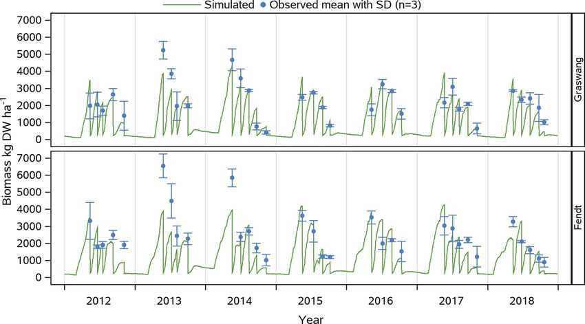
K. Petersen et al. European Journal of Agronomy 128 (2021) 126306
∑( )
ΔGDD = T− ΩT,BASE (3) growth and maintenance respiration. Growth respiration Rg (Eq. (12)) is
given by fixed factor (ΩYIELD ) depending on gross primary productivity
(GPP), which is provided by the photosynthesis model after Farquhar
The allocation of assimilated CO2 into roots (Eq. (4)) is given by:
et al. (1980) and Ball et al. (1987) that runs on top of PlaMox:
( ) ΩROOT × γcut
θroot = 1 − θstorage × (4) Rg = ΩYIELD × GPP (12)
ΩROOT × γcut + ΩLEAF + ΩSTEM
Growth respiration is assigned to the specific compartments
where the parameter γcut (Eq. (5)) increases the allocation to above depending on the current biomass allocation fraction θx . Maintenance
ground biomass before the first cut event following the concept of the respiration (Eq. (13)) for all plant compartments x ∈ {storage, root, leaf,
PROGRASS model (Lazzarotto et al., 2009). stem} is given by the compartment-specific biomass mx and a respective
{
ΩCUT , first cut event maintenance respiration coefficient (Amthor, 2000):
γ cut = (5)
1 , after first cut event T− ΩT,REF
Rm.x = mx × ΩR,x × ftemp × 2 10 (13)
The share of the remaining assimilated carbon between leaf and stem
compartment (Eq. (6)) is determined fulfilling the following condition with the same response function for low temperature as for photosyn
between actual compartment biomass mx and species-specific allocation thesis and a general Q10 temperature dependency with increasing
parameters: temperature.
Non-respiratory plant carbon losses include root exudation and plant
mstem ΩSTEM
= (6) senescence. Root exudation is given as a fraction related to root respi
mleaf + mstem ΩLEAF + ΩSTEM
ration (Eq. (14)):
Carbon that has been allocated to the storage is translocated to other
Rm.x = ΩEXUDATE × Rg,root (14)
plant organs after defoliation events, e.g., cutting or grazing and at the
onset of the vegetation period. At such events, all carbon from the Plant senescence (Eq. (15)) is given by the maximum of a set of
storage is distributed according to current allocation factors. response functions fs,x with regard to drought (Eq. (16)), frost (Eq. (17))
In contrast to carbon, nitrogen is always instantaneously redis and plant age (Eq. (18)):
tributed according to the demands from the different plant compart ( )
Sx = max fs,drought, fs,frost , fs,age × mx (15)
ments. The demand of each plant compartment is given by the current
dry matter biomass and optimum nitrogen concentrations ΩNC,x (x ∈ {
with x ∈ {storage, root, leaf , stem}.
storage, root, leaf, stem}), which are assumed to be constant over time.
These response functions are:
Total plant nitrogen demand (Ndemand) at each time step is then given by
( ( ))
(Eq. (7)): ⎧
⎨ ΩSEN,DROUGHT × 1− min 1, ψ − ψ wilt
∑ , ψ > ψ wilt
fs,drought = ΩH2 O,SEN × ψ field − ψ wilt
Ndemand = mx × ΩNC,x , x ∈ {storage, root, leaf , stem} (7) ⎩
x 0, ψ ≤ ψ wilt
Leaf biomass and a species-specific parameter describing specific leaf (16)
area (ΩSLA ) determine the leaf area index that is needed by the Farquhar
in which the species-specific drought stress factor ΩH2 O,SEN is similarly
and Ball based calculation of photosynthesis. Photosynthesis is further
defined as compared to the drought influence on photosynthesis,
regulated by the activity of the Rubisco enzyme (arubisco ) (Eq. (8)):
{
ΩSEN,FROST × |T|, T < 0
arubisco = ΩRUBISCO × fp,drought × fp,temp × fp,nitrogen (8) fs,frost = (17)
0, T ≥ 0
with the species-specific maximum rubisco activity ΩRUBISCO and the
with the hourly resolved temperature T in the air and the soil for above-
response functions fp,x representing the influence of drought (Eq. (9)),
and belowground senescence, respectively.
temperature (Eq. (10)) and nitrogen (Eq. (11)) on photosynthesis,
respectively: fs,age = ΩSEN,AGE (18)
⎧ ( )
ψ − ψ wilt
⎨ min 1, , ψ > ψ wilt 2.2.4. MeTrx
ΩH2 O × ψ field − ψ wilt (9)
The MeTrx model simulates soil carbon and nitrogen turnover and
fp,drought =
⎩
0, ψ ≤ ψ wilt the associated processes humification, mineralization, nitrification,
denitrification and ammonia volatilisation (Kraus et al., 2015). These
with the soil water content ψ , the wilting point ψ wilt , the field capacity processes are key for the simulation of inorganic nitrogen substrate
ψ field and species-specific drought stress factor ΩH2 O , availability (NH4, NO3) for plant uptake and microbial driven produc
⎧ ( ) tion and emissions of C (CO2) and N (NO, N2O, N2) emissions as well as
⎨ max 1, T − 0.8 ΩLIMIT , T < ΩLIMIT
⎪
other loses such as NO3 leaching and NH3 emissions. In addition to
fp,temp = 0.2 ΩLIMIT (10)
⎪
⎩ substrate availability (usually in form of Michaelis-Menten kinetics), all
1, T ≥ ΩLIMIT microbial processes depend on soil moisture and soil temperature,
which are provided by above-described sub-models as well as the model
with hourly resolved air temperature T and a species-specific critical
input quantities pH and soil texture.
temperature ΩLIMIT below which photosynthesis is inhibited,
cN,LEAF ΩNDEF,LEAF
fp,nitrogen = (11) 2.3. Dynamic management module
ΩNC,LEAF
with the ratio of actual (cN,LEAF ) and optimum leaf nitrogen concentra For grassland simulations, the LandscapeDNDC management module
tion ΩNC,LEAF of leafs and an exponent describing the reduction of rubisco requires inputs for execution of cutting and manuring events and further
activity under nitrogen limitation (ΩNDEF,LEAF ). information on quantity and composition of the applied manure (see
Assimilated carbon via photosynthesis is partly metabolized by Section 2.4), which all were previously read from a user derived man
agement input file.
4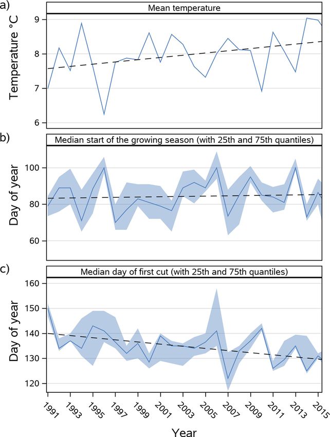
K. Petersen et al. European Journal of Agronomy 128 (2021) 126306
2.3.1. Description 1.) If the target biomass of the first cutting event is not reached after
The dynamic management model was developed from long term DOY 150, the first cut will be set at DOY 151.
field data (2012–2016) of a total of 22 biomass harvests (N = 3) (kg DM 2.) If the target biomass for all following cutting events is not
ha− 1) and respective cutting dates (DOY, day of the year) following reached within 55 days, they will be set at DOY 56 after the
actual farmers’ practice in the study region. These data were used to fit a previous cutting event.
linear regression to maximum standing biomass versus time, which al
lows to define a “target biomass” for executing a cutting event for any Since timing of manure events is highly related to timing of cutting
DOY. Hence, in the dynamic management model a cut is scheduled if the events, we defined the following rules regarding manure applications:
target biomass at a given DOY exceeds the threshold given by the
regression equation (Fig. 1). 1.) The first manure event is scheduled at the start of the growing
To calculate the target biomass for each cutting event we differen season as simulated by the vegetation sub-model but only at times
tiated between a site-specific regression approach (Graswang r2 = 0.39, without snow cover or frozen soil. Due to national legislation
p < 0.001; Fendt r2 = 0.57, p < 0.001) directly derived from field data (Achilles et al., 2018) manure events in any case are not sched
(target biomass = m ∗ DOY + b) and a general approach that can be uled before the 1st of February.
applied for intensive grasslands in the pre-alpine study region in the 2.) All other manure applications are scheduled within 7 days after
absence of detailed yield data (app. 500− 1000 m.a.s.l.). For the latter, in respective cutting events on the first day without heavy rain (<
addition to biomass harvest data of Graswang (864 m.a.s.l.) and Fendt 5 mm). Note that due to regional farmers practice and according
(595 m.a.s.l.) we also used further data of the TERENO site Rottenbuch to recommendations from extension services no manure is
(769 m.a.s.l.; 47◦ 43′ 49.152′ ’ N lat., 10◦ 58′ 14.844′ ’ E lon., Table 1). applied after the second cut. In line with legislation driven limi
We calculated the relative contribution (in %) of each cutting event to tation of fertilization rates to ≤ 170 kg N ha− 1 yr− 1 (Achilles
the annual biomass production which continuously decreased with et al., 2018) for the reduced nitrogen scenario, manure events are
number of cuts (r2 = 0.55, p < .0001; see Fig. S2). These relative con scheduled only before the first cutting and after the first and the
tributions can be translated into biomass thresholds by multiplying them third cutting event.
with the expected annual biomass production of a given grassland site,
which is set as an additional input parameter for the dynamic man 2.3.2. Calibration and validation
agement model of LandscapeDNDC. This value can either be derived First, we examined the capability of the site-specific and the general
from available measurements or alternatively from a regression model regression model to reproduce the field data management at Graswang
estimating annual yields (AGB in dt dry matter ha− 1 yr− 1) of intensively and Fendt. To do so we split the available data into a calibration
(4–5 cuts) used grasslands depending on elevation (h in m.a.s.l.) (Eq. (2012–2014) and a validation (2015–2018) period and ran simulations
(19)) as derived from managed grassland systems in Switzerland with weather data from on-site climate stations (see Section 2.4 for a
(Richner and Sinaj, 2017). detailed description of climate, soil and vegetation model inputs).
We further tested the dynamic management module for its capability
AGB = 159 − 0.058 ∗ h (19)
to simulate the timing of the first cut and the start of the growing season
We compared results from this function considering respective ele as given by phenological data routinely recorded by the German
vations of the three study sites Graswang, Rottenbuch and Fendt and Weather Service (DWD, Kaspar et al., 2014). Observations from 59 DWD
found only minor deviations of − 1.8 % to − 7.1 % from the field sites were available regarding the day of greening (equal to the start of
measurements. the growing season) i.e. 25 % of the grassland canopy characterized by
If the target biomass is not reached after a given time (day of the fresh green leaves, while data from 53 DWD sites were available
year: DOY), further rules are considered (see also Fig. 1), which also regarding the day of first cut in the Bavarian pre-alpine study region
evolve from field data and reflect farmer’s decision-making under un (48.05–47.56 latitude and 12.60–10.02 longitude and 500–1000 m.a.s.
favorable grassland growth conditions such as drought or cold spring: l.) between 1991 and 2016.
For more detailed testing of the general regression approach, we
Fig. 1. Scheme of rule sets of the dynamic management model; “default value” highlights a parameter which can be changed with the input file; DOY = day of the
year; Daysbetween = maximum count of days between two cuts; Tmin = daily minimum temperature (C◦ ); start of the growing season as simulated by the vegetation
sub-model.
5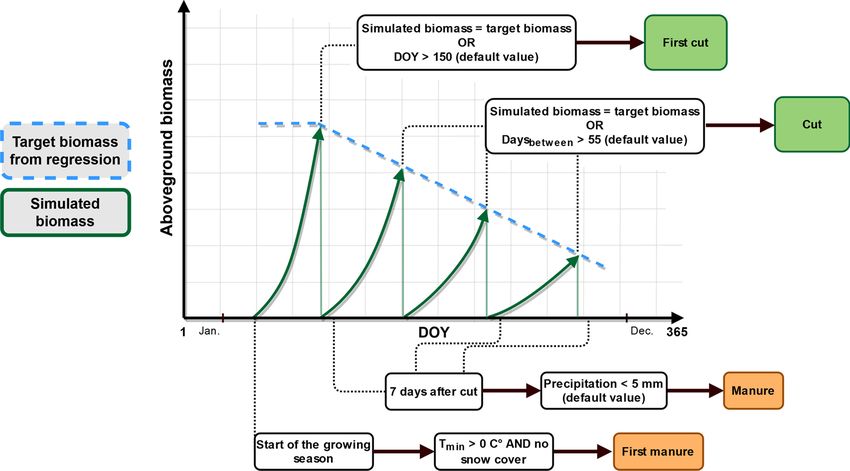
K. Petersen et al. European Journal of Agronomy 128 (2021) 126306
compared the simulated first cut and start of the growing season with often not available in this detail (Kipling et al., 2016; Luostarinen et al.,
observations of three phenological DWD sites representing different 2018), we conducted the following numerical experiments:
elevation levels (Table 1). Further selection criteria were completeness
of phenological time series and availability of weather data from nearby i) for an overall evaluation of LandscapeDNDC grassland biomass
DWD climate stations. Eventually, the following three sites were predictions (2012–2018) we used real time dates of single cutting
selected: 1) phenological site Nesselwang (47◦ 37′ 0.12′ ’ N lat., 10◦ 30′ and manuring events and measurements of manure composition
0′ ’ E lon., 870 m.a.s.l.) with DWD climate station Oy-Mittelberg (with annual fertilization rates ranging between 182 and 248 kg
(8.56 km distance, 47◦ 38′ 10.32′ ’ N lat., 10◦ 23′ 21.12′ ’ E lon., 885 m. N ha− 1 yr− 1);
a.s.l., 7.43 ◦ C MAT, 1589 mm MAP), 2) phenological site Memmingen ii) for climate change scenario simulations (2011–2100) with static
(47◦ 58′ 59.88′ ’ N lat., 10◦ 10′ 59.88′ ’ E lon., 600 m.a.s.l.) with DWD management settings we used mean cutting and manuring dates
climate station Memmingen (3.34 km distance, 47◦ 58′ 55.2′ ’ N lat., 10◦ of 2012–2018 (i.e. 4 cuts and 4 manure events, the latter equal to
8′ 18.24′ ’ E lon., 615 m.a.s.l., 8.49 ◦ C MAT, 964 mm MAP), 3) pheno 192 kg N ha− 1 yr− 1);
logical site Unterhausen (47◦ 52′ 0.12′ ’ N lat., 11◦ 9′ 0′ ’ E lon., 550 m.a.s. iii) for climate change scenario simulations (2011–2100) with dy
l.) with DWD climate station Raisting (5.73 km distance, 47◦ 54′ 32.76′ ’ namic management we derived cutting and manure events on the
N lat., 11◦ 6′ 17.28′ ’ E lon., 553 m.a.s.l. from 01.01.1994 to 31.01.1999, fly of simulations with the dynamic management module for a
with 8.2 ◦ C MAT and 1007 mm MAP) and with DWD station Wielenbach scenario with previously common fertilization rates (200− 240 kg
(1.92 km distance, 47◦ 52′ 57.72′ ’ N lat., 11◦ 9′ 27.36′ ’ E lon., 550 m.a.s. N ha− 1 yr− 1) and a scenario with reduced nitrogen fertilization (≤
l. from 01.02.1999 to 31.01.2016, with 8.74 ◦ C MAT and 987 mm MAP). 170 kg N ha− 1 yr− 1) following changes in legislation in 2018 (see
Since no detailed soil input for these sites were available we also Section 2.3, Achilles et al., 2018).
initialized all three sites with soil characteristics of the Graswang site
(see Section 2.4). For derivation of the average yearly biomass, we used Note that for ii) and iii) manure characteristics were represented by
the formula for intensively managed grasslands described in Section means of measurements of 2012 to 2016. For the limited nitrogen sce
2.3.1. nario only, we slightly adjusted total carbon and nitrogen loads per
event to achieve a maximum of 170 kg N ha− 1 yr− 1.
2.4. LandscapeDNDC model simulations
2.4.2. Soil and vegetation
The simulated development of aboveground biomass, soil carbon LandscapeDNDC allows a flexible vertical parameterization of the
and nitrogen dynamics depend on soil characteristics (Table 2), vege soil profile, depending on available measurements. Table 2 provides
tation growth parameters (Table S2), weather conditions as well as field essential soil input of LandscapeDNDC for the two simulated sites
management operations. Soil organic carbon and nitrogen is described Graswang and Fendt exemplarily for the top soil. In addition to data
by various empirical pool quantities representing different age and provided in Table 2, for our simulations we used further soil profile
decomposition classes. During a spin-up time of two years, pools of soil information of up to ten soil horizons down to 140 cm soil depth (Kiese
organic matter are brought into equilibrium with prevailing manage et al., 2018; see Table S1).
ment, soil and climate conditions. LandscapeDNDC was mainly developed and validated for single
species setups (mainly crops in arable systems) rather than for simu
2.4.1. Grassland management and simulations lating complex plant communities e.g. characterized by multiple plant
As mentioned in Section 2.3 management input requires in addition functional types, a main feature of many grassland ecosystems. There
to dates further information on quantity and composition of the applied fore, we simulated grass growth still by the single species approach but
manure. This includes the pH value, the total amounts of carbon (kg C in our case growth parameters represent mean values (see Table S2)
ha− 1), the C:N ratio and if available information on the partitioning of which originate from the calibration to the plant mixtures (see Section
nitrogen in fractions of NH+ 2.1) occurring at the two investigated grassland sites.
4 , NO3, UREA and dissolved organic nitrogen
(DON). For our study, information on cutting and manuring dates and
quantities were available for the time period 2012− 2018. Slurry 2.4.3. Weather data and climate change scenarios
composition was derived from analysis of slurry samples (N = 19; Raif LandscapeDNDC uses hourly or daily information on precipitation
feisen Laborservice, Ormont, Germany) of each fertilization event from [mm], minimum and maximum air temperature [◦ C] and global radia
2012 to 2016. Mean slurry carbon and nitrogen loads and pH values tion [W m− 2], which were available from weather stations operating
were 437 ± 130 kg C ha− 1 and 48 ± 10 kg N ha− 1 and 7.6 ± 0.4, since 2012 at the two study sites Fendt and Graswang. In case of daily
respectively. Given this information on grassland management, which is time resolution LandscapeDNDC uses well-established algorithms to
convert data in hourly time resolution (Berninger, 1994; Chow and
Levermore, 2007).
Table 2
Physical and chemical top soil (0–10 cm) characteristics of the grassland sites
Due to substantial biases in dynamically regionalized global climate
Fendt and Graswang; BD = bulk density, Corg = organic carbon content, Norg = models, particularly for precipitation in complex alpine terrains (Smia
organic nitrogen content, FC = field capacity, PWP = permanent wilting point, tek et al., 2016), site specific daily climate change scenarios (RCP 4.5
HC = hydraulic conductivity. and 8.5) for the time period of 2011–2100 were developed with the
Sites Graswang Fendt
stochastic weather generator LARSWG (Semenov and Barrow, 1997;
Depths 0–5 5 – 10 0–5 5 – 10 Semenov and Stratonovitch, 2010) which is a widely used tool in crop
modelling studies (e.g. De Bruijn et al., 2012; Lazzarotto et al., 2010).
BD [g kg− 1] 0.552 0.82 0.74 1.1
pH 4.9 7.1 5.1 6.6 LARSWG generates daily climate series of precipitation, global radiation
Corg [Weight-%] 10.02 5.81 6.79 4.35 and minimum and maximum air temperature based on probability dis
Norg [Weight-%] 1.001 0.67 0.66 0.48 tributions and correlations of long-term observed weather variables at
Clay fraction [%] 58.5 58.5 27.2 25.2 intended sites. Climate projections from global climate models (GCM)
Silt fraction [%] 35.1 35.1 40.3 40.3
Sand fraction [%] 6.4 6.4 32.5 34.5
are used to calculate climatic changes for a given site that are applied on
FC (pF 1.8) [Vol.-%] 52.0 52.0 50.0 46.0 these parameter distributions to create site specific climate change
PWP (pF 4.2) [Vol.-%] 22.1 22.1 23.5 23.5 scenario series (Semenov and Stratonovitch, 2010). To do so, LARSWG
HC [cm min− 1] 0.005 0.005 0.020 0.020 can make use of CMIP5 (Coupled Model Intercomparison Project Phase
Stone fraction [%] 1.0 1.5 0.0 3.8
5) global climate projections (Taylor et al., 2012) from which we
6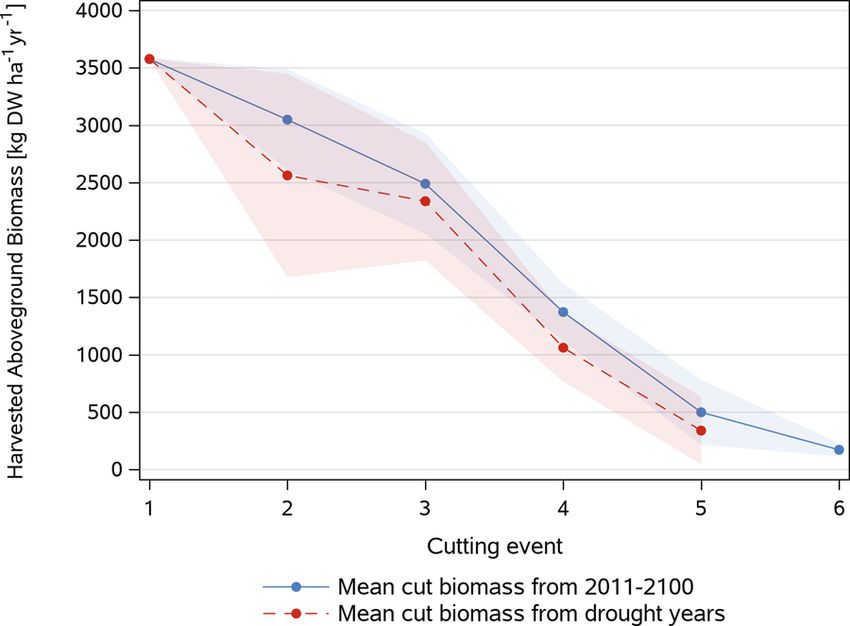
K. Petersen et al. European Journal of Agronomy 128 (2021) 126306
selected output of HadGEM2-ES, since it was shown to represent the 2.5. Statistical analysis
height- and latitude-dependent temperature and precipitation pattern
over the alpine region reasonably well (Zubler et al., 2016). In order to To evaluate model performance on biomass production, dynamically
assess the statistical uncertainty of the generated climate time series, simulated cutting dates and start of the growing season as well as to
LARSWG was used to generate ten different realizations for each site. analyze trends in the DWD phenological datasets, we used linear
Since climate stations in Graswang and Fendt have only been oper regression models and respective coefficients of determination (r2) as
ated since 2012, LARSWG calculations were informed instead by well as the concordance correlation coefficient (CCC) (Lin, 1989). Root
weather data from longer observation records of nearby stations of the mean square errors (RMSE) and normalized root mean square errors
German Weather Service (DWD). For Fendt, precipitation and air tem (NRMSE, =RMSE/average of observed values) were calculated to ac
perature data were taken from 17 years (2000–2017) time series of the count for differences between observed and simulated aboveground
DWD station Wielenbach (47◦ 53′ 2.4′ ’ N lat., 11◦ 9′ 28.8′ ’ E lon., 545 m. biomass harvests for the period of 2012− 2018. Additionally, for cutting
a.s.l., 9.16 km distance) with a MAP of 968 mm (Fendt site: 956 mm), dates in this reference period a paired t-test on the group mean values of
minimum MAT of 3.56 ◦ C (Fendt site: 3.54 ◦ C) and a maximum MAT of measured and simulated values was conducted (α = 0.05). To describe
14.68 ◦ C (Fendt site: 14.32 ◦ C). For Graswang, precipitation was derived changes in biomass harvest variability between years with climate
from a 15 years time series (2002–2017) of the DWD rainfall station change, we calculated coefficients of variation for the periods
Ettal-Graswang (47◦ 34′ 19.2′ ’ N lat., 11◦ 1′ 26.4′ ’ E lon., 872 m.a.s.l., 2011− 2040 and 2071− 2100 (CV = standard deviation / arithmetic
619.3 m distance) with a MAP of 1545 mm which is reasonable higher mean).
(+ 198 mm) than MAP measured on site. For the Graswang site air For tests on normality of the empirical distribution for any param
temperature was taken from the DWD station Garmisch-Partenkirchen eter, we used the Shapiro-Wilk test. In case of normal distributed data,
(47◦ 28′ 58.8′ ’ N lat., 11◦ 3′ 43.2′ ’ E lon., 719 m.a.s.l., 9.97 km dis we assessed correlation using the Pearson correlation coefficient. For
tance) but due to systematic differences in MAT (minimum MAT 2.65 ◦ C, non-normally distributed data, the Spearman rank test was used.
maximum MAT 13.94 ◦ C) these data were corrected using a linear All statistical analysis and figures were generated using SAS/STAT
regression of Graswang and Garmisch air temperature data for the years software, Version 9.4 of the SAS System for Windows. Copyright ©
2012 to 2016: TMAX Graswang = 0.9359 * TMAX Garmisch – 0.915 (r2 = 0.88) 2012− 2018 SAS Institute Inc. SAS and all other SAS Institute Inc.
and TMIN Graswang = 0.993 * TMIN Garmisch – 1.3523 (r2 = 0.91). product or service names are registered trademarks or trademarks of SAS
Global radiation was taken for both sites from DWD station Hohen Institute Inc., Cary, NC, USA.
peißenberg (47◦ 48′ 3.24′ ’ N lat., 11◦ 0′ 38.88′ ’ E lon., 977 m.a.s.l.,
25.8 km distance to Graswang, 5.24 km distance to Fendt). 3. Results
Within the RCP 4.5 scenario a mean annual temperature increase
within the vegetation period of maximum 1.4 ◦ C is predicted from 2011 3.1. Aboveground biomass simulations
to 2070 and from thereon less steep by up to 1.7 ◦ C in the year 2100
(Table 3). For RCP 8.5 a continuous temperature increase of 1.9 ◦ C Robust simulations of grassland biomass development and yields at
(Graswang and Fendt) until 2070 and of up to 4.4 ◦ C in 2100 are re respective cutting events are essential for the applicability of Land
ported. The mean annual precipitation for both sites for RCP 4.5 is scapeDNDC for evaluation of grassland functions under current and
slightly decreasing towards 2070 with a tendency to increase again after climate change conditions. Fig. 2 shows the temporal development of
2070 until 2100. For RCP 8.5 the precipitation further decreases after simulated and measured harvested biomass (n = 3) at cutting events
2070 which results in overall 107− 172 mm less annual precipitation at (2012− 2018) of LandsapeDNDC being parametrized with specific
the end of the simulation period compared to the first period between climate, soil and management information for the Fendt and Graswang
2011–2040. sites.
For all simulations under current climate conditions we set atmo Disregarding the year 2013 with exceptional high measured biomass
spheric CO2 concentrations to a fixed value of 400 ppm, while tran for the first two cuts in Graswang and Fendt and the first cutting event in
siently (yearly) increasing atmospheric CO2 concentrations were used Fendt in 2014, patterns and magnitude of the simulated biomasses were
for the climate change scenarios based on the datasets provided by mostly consistent with measurements. Statistical measures of the cali
Meinshausen et al. (2011), reaching maximum values of 538 ppm and bration (2012–2014) and validation (2015–2018) period were in the
936 ppm CO2 in 2100 in RCP 4.5 and RCP 8.5 scenarios, respectively. same range (Graswang: r2 = 0.62− 0.71, p < .0001; Fendt:
r2 = 0.64− 0.66, p < .0001) with the only exception in the calibration
period for Fendt with a higher RMSE value of 1127 kg DW ha− 1
(NRMSE = 38.6 %). Considering the complete simulation period of
seven years with a total of 32 cutting events resulted in RMSE of 720 and
Table 3
917 kg DW ha− 1 and r2 of 0.61 (p < .0001) and 0.52 (p < .0001) for
Average climatic conditions (± SD) in the vegetation period (March to October)
of the two sites Graswang and Fendt originating from 10 realizations of site Graswang and Fendt, respectively (NRMSE: Graswang = 31.7 %,
specific climate change scenarios generated by LARSWG and based on the Fendt = 37.1 %).
HadGEM2-ES climate projection over 30-year periods from 2011 to 2100.
T = temperature in ◦ C; PREC = precipitation in mm. 3.2. Dynamic management simulations
Site RCP Period T [ C]
◦
PREC [mm]
Fig. 3 shows the comparison of dynamically simulated and observed
Graswang 4.5 2011–2040 10.8 ± 0.5 1219 ± 148
2041–2070 12.1 ± 0.4 1165 ± 167
cutting DOY for the calibration period 2012–2014 and the validation
2071–2100 12.5 ± 0.3 1193 ± 168 period 2015− 2018. For both periods, the dynamic simulations accu
8.5 2011–2040 10.8 ± 0.5 1245 ± 161 rately represented the timing of cutting events (r2 = 0.89− 0.98). The
2041–2070 12.7 ± 0.6 1175 ± 156 performance of the general approach was only slightly lower than the
2071–2100 15.2 ± 0.4 1073 ± 153
performance of the site-specific approach, with a tendency in the cali
Fendt 4.5 2011–2040 13.2 ± 0.4 757 ± 117
2041–2070 14.6 ± 0.4 712 ± 119 bration period towards later simulated cuts for the warmer Fendt site
2071–2100 14.9 ± 0.2 752 ± 112 and earlier simulated cuts for the colder Graswang site after the third
8.5 2011–2040 13.2 ± 0.5 778 ± 111 cut. This also shows up by higher deviations of the slope, with values < 1
2041–2070 15.1 ± 0.6 741 ± 124 at Fendt and > 1 at Graswang, respectively. Group means of the cutting
2071–2100 17.6 ± 0.4 671 ± 109
DOY at 1st to 5th cuts were not significantly different from measured
7
K. Petersen et al.                                                                                                      European Journal of Agronomy 128 (2021) 126306

Fig. 2. Simulated and mean ± SD measured (n = 3) aboveground biomass (in kg DW ha− 1) during 2012 to 2018 at the two grassland sites Graswang (top) and
Fendt (bottom).

Fig. 3. Correlation of dynamically simulated and observed Day of Year (DOY) of cutting events for the calibration (2012 to 2014; a and b) and the validation (2015 to
2018; c and d) period with the site-specific (a and c) and the general regression approach (b and d), 1st = first cut; 2nd = second cut etc.

Table 4
Deviations of cutting events between simulations and observations during the period 2012 to 2018.
  Year                            2012             2013             2014              2015            2016             2017             2018             2012–2018

  Field data                      5                4                5                 4               4                5                5                32
  Graswang site-specific          –                +1               –                 –               +1               − 1              − 1              –
  Fendt site-specific             –                –                –                 +1              +1               –                –                +2
  Graswang general                –                +1               –                 +1              +1               –                –                +3
  Fendt general                   –                –                –                 –               +1               –                –                +1

                                                                                  8
K. Petersen et al. European Journal of Agronomy 128 (2021) 126306
values (t-test; p > 0.05) but due to error propagation deviations of differences of the temporal development between the RCP 4.5 and 8.5
simulations and field measurements increased with increasing number scenarios were smaller.
of cuts (Fig. 3).
At both sites, the simulated number of yearly cuts and the total 3.3.2. Validation of simulations against DWD phenological observations
number of cuts during the full 7-year simulation period match very well Compilation of data of the start of the growing season and first cut
with field observations (Table 4). Simulated counts of cutting events per from >50 sites of the phenological observation network of the German
year deviate by a maximum of ± 1 from observed data. Regarding all 32 Weather Service (DWD) located in the pre-Alpine study region revealed
cutting events, both site-specific and general simulations slightly over a significant trend towards earlier dates of first cuts from 1991 to 2016
estimated the number of cutting events by a maximum of three cuts. (r2 = 0.25, p < 0.05), following the trend of increasing mean annual air
In addition to the detailed validation of predicted cutting events with temperatures during this time period (correlation of first cutting dates
TERENO field data we compared LandscapeDNDC simulations also with and temperature; r = 0.72, p < .0001) (Fig. 6). A shift of 4.5–6.7 days
observations of three phenological sites of the German Weather Service (representing 25th and 75th percentiles) towards earlier first cuts be
(DWD), namely Nesselwang, Memmingen and Unterhausen. Fig. 4a tween two periods 1991− 2000 and 2007–2016 was observed. Refer
shows the correlation between simulated (general approach) and encing this to the mean temperature increase in the same period of
observed first cutting events for all three sites. Despite a pronounced +0.48 ◦ C results in an earlier timing of the first cut between 9.4–14.0
scattering of simulated and observed data, the correlation was signifi days per 1 ◦ C temperature increase.
cant (r = 0.47; p < 0.002). In 74 % of the cases the model predicted the Results of the RCP climate scenario simulations of LandscapeDNDC
first cut within ± 7 days of the observed date with a corresponding for an equally long period (2011− 2040) agreed well with these obser
RMSE of 7.8 days. The average difference between simulated and vations with a similar range of 9.1–16.9 days earlier first cutting dates
observed cuts was 2.2 ± 7.5 days. referenced to a temperature increase of 1 ◦ C (Table 5).
For the start of the growing season (Fig. 4b) a stronger correlation In contrast to the shifts observed for first cutting dates, the DWD
(r = 0.53, p < 0.001) between simulated and observed dates was found, phenological observations do not show a clear trend of changes in the
but the mean deviation of − 13.5 ± 15.7 days revealed a bias towards an timing of the start of the growing season (Fig. 6) with median values
earlier simulated start of the growing season as compared to observa spreading between DOY 70 and 100. Interestingly, and following DWD
tions. As a result, only 40 % of the simulated values were within ± 7 days observations LandscapeDNDC RCP scenario simulations also do not
of the observed dates, and the RMSE was also higher (20.7 days). show a clear trend until approximately 2030. Nevertheless, for both
sites, the simulated start of the growing season is about up to 20 and 30
3.3. Grassland management predictions under climate change conditions days earlier in 2080 and stabilize towards 2100 for the RCP 4.5 and 8.5
scenario, respectively (Fig. 5).
3.3.1. Shift of the start of the growing season and the first cut
As the validation results for the reference period did not show any 3.3.3. Influence on number of yearly cuts
significant differences in model performance between the site-specific Trends towards an earlier start of the growing season and first cutting
and the general dynamic management approach, we present here only dates as simulated by the dynamic management routine of Land
data of the general approach. Fig. 5 depicts the temporal progression of scapeDNDC influenced also the total number of cutting events per year.
the start of the growing season and the day of the first cutting event of For the > 200 kg N dynamic simulations the number of cuts increased at
simulations based on the RCP 4.5 and RCP 8.5 climate change scenarios both sites and in both RCPs from alternating between four and five cuts
for the Fendt and Graswang sites. (2011− 2035) to regularly five cuts after 2035. For the RCP 8.5 scenario
In both RCP scenarios with progression of time a clear trend towards from 2080 onwards, even six cuts were simulated at the warmer Fendt
an earlier simulated start of the growing season and first cutting events site and after 2090 likewise for the colder Graswang site. Within the
are evident (Fig. 5). Simulated first cutting events at the higher elevation reduced N scenarios, four cuts were constantly simulated for both sites
site Graswang changed from DOY 130 to 105 in the RCP 4.5 scenario and between 2011 and 2035 and a slower increase to a maximum of five cuts
to DOY 85 in the RCP 8.5 scenario. For the warmer site Fendt compa thereafter. Five cuts were continuously simulated from 2045 at the
rable temporal patterns and differences between RCP 4.5 and the RCP earliest for Fendt RCP 8.5 and from 2080 at the latest for Graswang RCP
8.5 were observed, however DOYs of the first cutting events were in both 4.5 without a predicted increase towards six cutting events.
scenarios approximately 10 days earlier as compared to Graswang.
Compared to changes in the dates of the first cutting event, at both sites, 3.3.4. Grassland biomass production under climate change conditions
simulated changes of the start of the growing season were less early and The previous findings of dynamic grassland management simulations
Fig. 4. Correlation of simulated (general approach) and observed (a) first cutting events and (b) start of the growing season for phenological German Weather
Service (DWD) stations Nesselwang, Memmingen and Unterhausen.
9K. Petersen et al. European Journal of Agronomy 128 (2021) 126306
Fig. 5. Simulated day of first cut and start of the growing season at Graswang and Fendt sites for RCP 4.5 and 8.5 emission scenarios. Shown are median with 5-year
moving average (solid lines) and band of 25th and 75th percentiles originating from 10 realizations of site specific climate change scenarios generated by LARSWG
and based on the HadGEM2-ES climate projection.
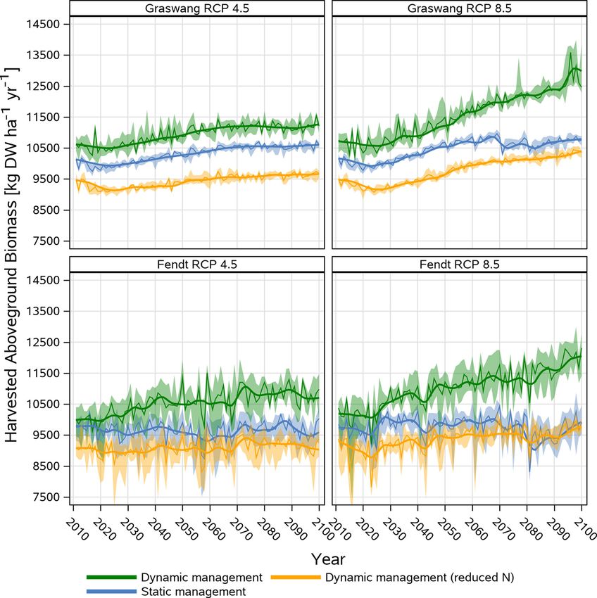
showed that climate change beside earlier execution of the first cut 2011− 2040 and 2071− 2100. In the RCP 8.5 scenario grassland yield
result in increasing number of cuts and associated manure events, fea increases under dynamic non-reduced N management at Fendt were
tures which cannot be reflected by static management or if annual similar to Graswang. This was not the case for the static and dynamic
fertilization rates are restricted to 170 kg N ha− 1 as required by legis reduced N management which both showed even a decreasing trend
lation since 2018. from 2060 onwards. The yield increase in RCP 8.5 for the dynamic non-
For Graswang and the RCP 4.5 scenario, the dynamic reduced N reduced N management resulted in a mean biomass of 11606 kg DW
scenario showed lower biomass yields of about 1000–1600 kg DW ha− 1 ha− 1 yr− 1 for the 2071− 2100 period, which is about 1170 kg higher as
yr− 1 as compared to the higher loads of N fertilization under static and compared to the start of the simulation period (2011− 2040) and about
the dynamic management. Within RCP 8.5 simulations, the yield dif 2000 kg DW ha− 1 yr− 1 higher than the mean biomass associated with
ferences between the static and the reduced N management decreased in static (9642 kg DW ha− 1 yr− 1) and dynamic non-reduced N (9557 kg DW
the 2071− 2100 period (< 500 kg DW ha− 1 yr− 1) while the difference to ha− 1 yr− 1) management operations for 2071− 2100.
the dynamic non-reduced N scenario increased to 2159 kg DW ha− 1 At the warmer Fendt site simulated yields showed overall higher
yr− 1. Overall, climate change induced increases of yields of the three differences across years (Fig. 7) which is also documented by higher
management scenarios were about 500 kg DW ha− 1 yr− 1 between the coefficients of variation ranging between 3–5 % at Graswang and 7–10
period of 2011− 2040 and 2071− 2100 in RCP 4.5 and 8.5, except for the % at the Fendt site. With regard to climate change at both sites the
dynamic management and the RCP 8.5 scenario where yield increases variability of yields were not different for the period 2011− 2040 and
for the same period of time with 1600 kg DW ha− 1 yr− 1 were much 2071− 2100 neither for RCP 4.5 nor RCP 8.5. Nevertheless, as shown in
higher (Fig. 7). Fig. 8 yields of occasional drought years defined by < 550 mm growing
As compared to Graswang lower differences (500 kg DW ha− 1 yr− 1) season (March-October) precipitation were about 15 % lower than in
between the static and dynamic reduced N scenario were simulated for non-drought years with a mean growing season average of
Fendt in the RCP 4.5 and RCP 8.5 scenario for the period 2011− 2040 730 ± 123 mm. Thereby yields for the first cut were equal to non-
which further decreased in the period 2071− 2100. In contrast to Gras drought years but overall lower yields were simulated for the second
wang, climate change as predicted by RCP 4.5 did not lead to increasing to the fifth cut while unfavorable growth conditions in drought years did
grassland biomass under static and the dynamic reduced N manage not support a sixth cut as simulated for non-drought years.
ment, while for the dynamic non-reduced N management increases of
about 650 kg DW ha− 1 yr− 1 were predicted during both periods
10You can also read