Assessment of probability distributions and analysis of the minimum storage draft rate in the equatorial region - Natural Hazards and Earth System ...
←
→
Page content transcription
If your browser does not render page correctly, please read the page content below
Nat. Hazards Earth Syst. Sci., 21, 1–19, 2021
https://doi.org/10.5194/nhess-21-1-2021
© Author(s) 2021. This work is distributed under
the Creative Commons Attribution 4.0 License.

Assessment of probability distributions and analysis of the
minimum storage draft rate in the equatorial region
Hasrul Hazman Hasan1 , Siti Fatin Mohd Razali1 , Nur Shazwani Muhammad1 , and Firdaus Mohamad Hamzah2
1 Department of Civil Engineering, Faculty of Engineering & Built Environment,
Universiti Kebangsaan Malaysia, Bangi, 43600, Malaysia
2 Department of Engineering Education, Faculty of Engineering & Built Environment,

Universiti Kebangsaan Malaysia, Bangi, 43600, Malaysia

Correspondence: Siti Fatin Mohd Razali (fatinrazali@ukm.edu.my)

Received: 2 April 2020 – Discussion started: 22 April 2020
Revised: 1 November 2020 – Accepted: 9 November 2020 – Published: 4 January 2021

Abstract. Rapid urbanization in the state of Selangor,             cember to be a critical period in river water storage to sustain
Malaysia, has led to a change in the land use, physical prop-      the water availability during low flow in a 10-year occurrence
erties of basins, vegetation cover and impermeable surface         interval. These findings indicated that hydrological droughts
water. These changes have affected the pattern and processes       have generally become more critical in the availability of
of the hydrological cycle, resulting in the ability of the basin   rivers to sustain water demand during low flows. These re-
region to store water supply to decline. Reliability on water      sults can help in emphasizing the natural flow of water to
supply from river basins depends on their low-flow charac-         provide water supply for continuous use during low flow.
teristics. The impacts of minimum storage on hydrological
drought are yet to be incorporated and assessed. Thus, this
study aims to understand the concept of low-flow drought
                                                                   1   Introduction
characteristics and the predictive significance of river storage
draft rates in managing sustainable water catchment. In this       Droughts are long-term natural disaster phenomena result-
study, the long-term streamflow data of 40 years from seven        ing from less-than-average precipitation causing significant
stations in Selangor were used, and the streamflow trends          damages to a wide variety of sectors, affecting large regions.
were analyzed. Low-flow frequency analysis was derived us-         The rapid development of the world now sees an increase in
ing the Weibull plotting position and four specific frequency      population, and climate change tends to increase drought oc-
distributions. Maximum likelihood was used to parameter-           currences (Bakanoğullari and Yeşilköy, 2014; Tigkas et al.,
ize, while Kolmogorov–Smirnov tests were used to evaluate          2012). Droughts have considerable economic, societal and
their fit to the dataset. The mass curve was used to quan-         environmental impacts. Droughts can typically be classified
tify the minimum storage draft rate required to maintain the       into four types, depending on the different kinds of impacts
50 % mean annual flow for the 10-year recurrence interval of       of drought in different areas: meteorological, hydrological,
low flow. Next, low-flow river discharges were analyzed us-        agricultural and socio-economic (Hasan et al., 2019; Tri et
ing the 7 d mean annual minimum, while the drought event           al., 2019). Any type of drought is dynamic and defined by
was determined using the 90th percentile (Q90 ) as the thresh-     various characteristics such as frequency, severity, duration
old level. The inter-event time and moving average was em-         and magnitude. This study mainly focuses on hydrological
ployed to remove the dependent and minor droughts in de-           drought. The related hydrological aspects, including low wa-
termining the drought characteristics. The result of the study     ter levels and decreased groundwater recharge, are more di-
shows that the lognormal (2P) distribution was found to be         rectly affected by the hydrological-drought impacts.
the best fit for low-flow frequency analysis to derive the low-
flow return period. This analysis reveals September to De-

Published by Copernicus Publications on behalf of the European Geosciences Union.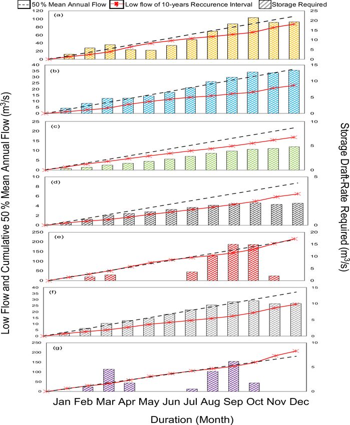
2                         H. H. Hasan et al.: Assessment of probability distributions and the minimum storage draft rate

   Extreme drought can cause significant water cycle imbal-        Blöschl, 2006, 2007; Liu et al., 2016). The influences on hy-
ances that alter the processes of precipitation and evapo-         drological drought are not restricted to the external variables
ration; the circulation of atmospheric water vapor; and the        such as climatic and watershed variables and should not be
availability of soil moisture, which results in a low volume       disregarded for anthropogenic activities in the form of land
of water in streams, rivers and reservoirs. The equilibrium        use modification, reservoir control, irrigation, and water ex-
between both the water that is taken out for supply and that       traction or withdrawal (Hatzigiannakis et al., 2016; Richter
is substituted by surface runoff must be maintained. A critical    and Thomas, 2007; Sun et al., 2018; Toriman et al., 2013).
issue arises when there is a dry season and there is no esti-         In the event that the low flow of the river is sufficient to
mated water excess. Under such conditions, water shortages         meet the water demand, the storage may be utilized to in-
can happen even though the dry season is not too extreme.          crease the guaranteed water supply. The hydrological aspects
Human activities and poor management of water resources            which must be considered are the amount of storage neces-
can lead to water scarcity, which could be exacerbated by          sary to sustain a given draft rate and the associated risk of
drought. In certain regions, water consumption increases the       insufficient storage to meet this draft rate. The relationship
severity of water scarcity and triggers water shortage events      between inflow, storage and draw-off is complex. Significant
in regions that are relatively well endorsed with water re-        sources of error are associated with frequency analysis. Er-
sources (Wada et al., 2013).                                       ror in frequency analysis is due to fitting the type of extreme-
   Hydrological drought is a natural event with streamflow         value distribution to low-flow series and uncertainties associ-
deficits in duration and volume (Kubiak-Wójcicka and Bak,    ˛     ated with assigning recurrence intervals for cumulative prob-
2018). In a hydrological drought, not every low-flow occur-        abilities to the events in series. Drainage basin stores are sur-
rence can be called a drought, and several low flows can form      faces of significant quantities of water that may regulate the
one hydrological drought (Teegavarapu et al., 2019). It is not     rate at which input feeds through to the output. Channel stor-
advisable to equate hydrological drought with low flow or          age is the volume of water contained within banks of the river
other related hazards. Low flow is a term that is often used,      that will operate as a water store between its initial input and
referring to low-flow discharge. Low flow is often defined         ultimate output (Griffiths and Clausen, 1997).
by a minimum annual series which does not reflect hydro-              This study was conducted in the state of Selangor on the
logical drought in all years. Fleig et al. (2006) distinguished    western coast of Peninsular Malaysia to evaluate and investi-
between hydrological-drought and low-flow characteristics.         gate the hydrological-drought characteristics using historical
For some specific purposes, the main feature of drought is         streamflow data. High demand for water that can accommo-
said to be the water deficit. Low flows are usually observed       date the daily water consumption of the population due to
during a drought, but they only feature one aspect of the          rapid growth, as well as the lack of rain, has caused disrup-
drought, namely the magnitude of drought. Low-flow anal-           tions of water supply in Selangor (Khalid, 2018; Kwan et al.,
ysis is described as analyses that attempt to understand the       2013; Ngang et al., 2017). Water shortages associated with
short-term physical development of flows at a point along a        the El Niño–Southern Oscillation (ENSO) incident impacted
river. The minimal annual n d average discharge is the most        parts of Malaysia, including Selangor (Sanusi et al., 2015;
widely used low-flow index.                                        Zainal et al., 2017). Drought disasters have hit several re-
   Water availability in many areas is becoming less pre-          gions in Malaysia, especially in the Klang Valley, Selangor;
dictable due to climate change. More significant periods of        Penang; and several other places such as Kedah, Kelantan,
drought and higher temperature are projected to affect the         Sarawak and Sabah (Chan, 2012). The problems of water
rainfall distribution and river flow used for water availability   shortage and drought in Malaysia were recorded as early as
causing deleterious effects on water supply. The watershed         1951, when it occurred for 29 months in the Langat River
also plays a significant role in the propagation of drought        basin (Chan, 2012). After that episode, the drought disaster
and affects procedures such as pooling, lagging and length-        continued to hit Malaysia with the Klang Valley water cri-
ening (Fleig et al., 2006; Sarailidis et al., 2019). Some re-      sis in February–May 1998; the water shortage continued in
search further explored the specific functions of climate con-     Hulu Langat, Selangor, in 2002 (Ithnin, 2014). This drought
trol and watershed influence in regulating features of hydro-      has caused the water level in some water dams in Peninsular
logical drought, and the findings are largely based on spatial     Malaysia to reach critical levels, like what happened in the
scales (Austin and Nelms, 2017; Barker et al., 2016; Liu et        1997–1998 drought episode (Lee et al., 2018). Consequently,
al., 2012; Zarafshani et al., 2016; Zhu et al., 2018). Gener-      the characteristics of hydrological drought must be identified,
ally, the duration of hydrological drought and the quantity of     and the effects of hydrological drought must be quantitatively
the deficit are more climate-related than watershed-related.       evaluated. Studies conducted by Iqbal et al. (2016), Azadi et
However, watershed features such as geology, region, slope         al. (2018), and Tigkas et al. (2012) have highlighted the is-
and groundwater regime perform a significant part in regu-         sue of hydrological drought and its impact on agricultural,
lating the duration of hydrological drought and the quantity       socio-economic and streamflow in the watershed (Azadi et
deficit for the regional scale, where the climate is presumed      al., 2018; Iqbal et al., 2016; Tigkas et al., 2012).
to be relatively constant (Gianfagna et al., 2015; Laaha and

Nat. Hazards Earth Syst. Sci., 21, 1–19, 2021                                          https://doi.org/10.5194/nhess-21-1-2021
H. H. Hasan et al.: Assessment of probability distributions and the minimum storage draft rate                                  3

   The hydrological drought was referred to as the most crit-     2   Study area
ical aspect of drought, with significantly reduced streamflow
and lower water storage in the river system (Hasan et al.,        The scope of this study covers the entire streamflow station
2019). Because of this, the storage rate for each river should    in the state of Selangor. Selangor covers an area of 8104 km2
be established to ensure the minimum storage for water sup-       and is located on Peninsular Malaysia’s western coast. Se-
ply requirement during low flow and drought in the coming         langor’s water supply system not only covers the state of
years sufficient to accommodate consumers’ water demand.          Selangor but also supplies water to the Kuala Lumpur and
Some relevant research questions in the investigation of hy-      Putrajaya areas (Sakke et al., 2016a). The basins of the Lan-
drological drought are:                                           gat, Klang and Selangor rivers are the main river basins in
                                                                  Selangor. There are also three other river basins in Selan-
 1. Is there a decreasing pattern in the streamflow in the        gor, which are the basins of the Buloh, Bernam and Tengi
    Selangor region, and is the streamflow trend the same         rivers. Table 1 shows the locations and characteristics of all
    throughout the year?                                          streamflow gauging stations involved in this study. Langat
                                                                  and Semenyih dams, located at the upper reaches of the Lan-
 2. What is the likelihood of frequency of low-flow condi-        gat River (Elfithri et al., 2018), serve to regulate the raw wa-
    tions in the river system in the state of Selangor?           ter supplied to treatment plants downstream. The main trib-
 3. What is the minimum required storage draft rate based         utaries of Selangor’s rivers are the Sembah, Kanching, Ker-
    on monthly time series?                                       ling, Rawang and Tinggi rivers. There are two dams, namely
                                                                  the Selangor and Tinggi dams, in the Selangor River basin.
 4. How well does the threshold level method perform in              The state of Selangor is characterized by its geographical
    determining the hydrological-drought characteristics?         position, which lies near the equatorial climate that is warm
                                                                  and humid all year (Lassen et al., 2004). The average annual
The primary purposes of this study are:                           temperature varies between 27 and 30 ◦ C, and the average
                                                                  annual relative humidity is between 70 % and 90 % (Lee et
 1. to arbitrate the trend analysis of streamflow for 40 years;
                                                                  al., 2013). The equatorial climatic regions are influenced by
 2. to determine the best-fitted distribution of probability      two monsoons: the southwest Indian monsoon and the north-
    for each station for low-flow frequency analysis;             east Asian monsoon, which result in two rainy seasons with
                                                                  a significant number of storms, resulting in a mean annual
 3. to determine the minimum storage draft rates in seven         rainfall of about 2500 mm (Mamun et al., 2010). Even though
    catchments in the Selangor region in Malaysia;                Selangor is located in the humid region, it occasionally en-
                                                                  counters drought periods. Dry spells, low rainfall and high
 4. and to evaluate the hydrological-drought characteristics,     soil impermeability due to population growth are the leading
    including severity, duration and magnitude.                   causes of low-flow events. A stream’s regime can display one
This study is essential to understand the concept of low-         or more low-flow events depending on the climate. Two rainy
flow drought characteristics and the predictive significance of   and two dry seasons represent the equatorial climate, and the
river storage draft rates in managing sustainable water catch-    two streamflow regimes have two corresponding periods of
ment. The findings are useful for designing strategies to sus-    high flow and low flow. Figure 1 shows the seven streamflow
tain the variability of flow and can be used to implement risk    gauging stations involved in this study with four streamflow
management policies. Thus, this study consists of four types      gauging stations located at the Langat River basin at Dengkil,
of analyses, which are:                                           Kajang, Semenyih and Lui. There is also streamflow gauging
                                                                  station at Rantau Panjang for the Selangor River basin, Tan-
 1. the analysis of daily streamflow trend for a 40-year time     jung Malim and Jambatan Sekolah Kebangsaan Cina for the
    series using the Mann–Kendall test, Sen’s slope test,         Bernam River basin, respectively (Department of Irrigation
    distribution-free test (CUSUM; cumulative sum control         and Drainage Malaysia, 2011). The headwater of the Lan-
    chart) and Pettitt test;                                      gat River basin starts from the northeast of the basin, flows
                                                                  to the southwest and joins the Semenyih River. The Langat
 2. a low-flow frequency analysis on annual minimum flow          and Semenyih dams, the Selangor and Tinggi dams, are lo-
    using the best-fitting distributions;                         cated at the upper reaches of the Langat River and Selangor
                                                                  River basins, respectively, (Elfithri et al., 2018) to regulate
 3. the determination of minimum storage draft rates nec-
                                                                  the quantities of streamflow to the treatment plants.
    essary to ensure the sufficiency of water supply during
    low-flow periods;

 4. and an analysis of hydrological-drought characteristics
    determined using a fixed drought threshold at the 90th
    flow percentile.

https://doi.org/10.5194/nhess-21-1-2021                                        Nat. Hazards Earth Syst. Sci., 21, 1–19, 2021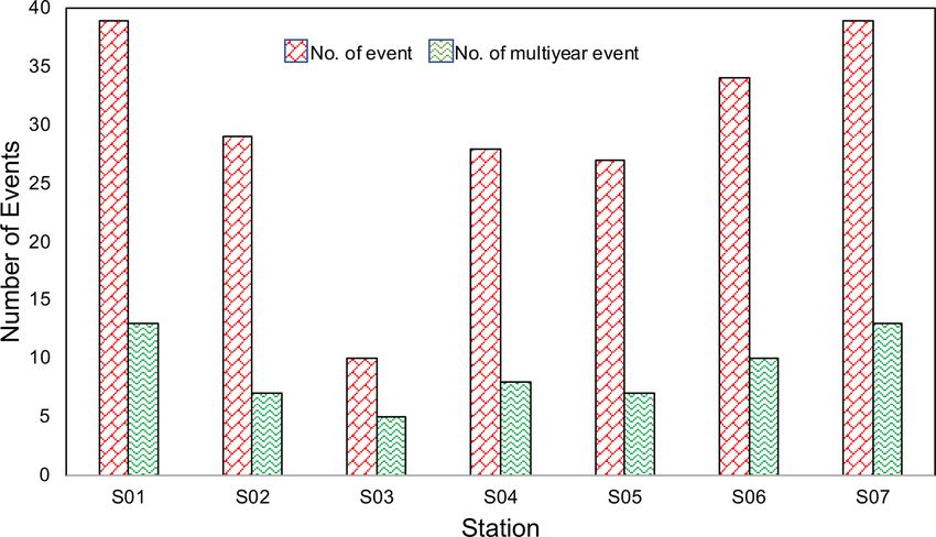
4                          H. H. Hasan et al.: Assessment of probability distributions and the minimum storage draft rate

Table 1. The characteristics of streamflow gauging stations in Selangor. WGS: World Geodetic System.

    Station   Station ID   River name                              River         Location coordinate (WGS)           Area    Affected by
    no.                                                            basin                                            (km2 )   reservoir
    S01       2816441      Langat River at Dengkil                 Langat       02◦ 510 2000 N    101◦ 400 5500 E    1240    No
    S02       2917401      Langat River at Kajang                  Langat       02◦ 590 4000 N    101◦ 470 1000 E     380    Yes
    S03       2918401      Semenyih River at Kampung Rinching      Langat       02◦ 540 5500 N    101◦ 490 2500 E     225    Yes
    S04       3118445      Lui River at Kampung Lui                Langat       03◦ 100 2500 N    101◦ 520 2000 E      68    No
    S05       3414421      Selangor River at Rantau Panjang        Selangor     03◦ 240 1000 N    101◦ 260 3500 E    1450    Yes
    S06       3615412      Bernam River at Tanjung Malim           Bernam       03◦ 400 4500 N    101◦ 310 2000 E     186    No
    S07       3813411      Bernam River at Jambatan Sekolah        Bernam       03◦ 480 1500 N    101◦ 210 5000 E    1090    No
                           Kebangsaan Cina

                                                                      tained from the flow duration curve (FDC), and 90th per-
                                                                      centiles were selected for drought analysis. Finally, the char-
                                                                      acteristics of hydrological drought were analyzed, including
                                                                      drought events, durations and drought deficits in seven wa-
                                                                      tershed catchments. The summary of the whole methodology
                                                                      analysis is depicted in Fig. 2. The following sections eluci-
                                                                      date the specific components incorporated into the method-
                                                                      ological framework.

                                                                      3.1     Streamflow trend analysis

                                                                      The mean annual streamflow was analyzed for significant
                                                                      trends, and distribution changes are discussed. The trend
                                                                      slope is measured using the Sen’s slope estimator, which pro-
                                                                      duces the magnitude of change in trends. Finally, using the
                                                                      CUSUM test, the change points were defined in the long-
                                                                      term streamflow results, and the changes in streamflow be-
                                                                      fore and after the change points were examined using the
Figure 1. River basin and streamflow station in Selangor.             Pettitt test. All analyses were conducted at seven stations to
                                                                      recognize the spatial variability based on historical stream-
                                                                      flow pattern change. The Mann–Kendall test and Sen’s slope
3   Methodology                                                       test are the most commonly used non-parametric trend anal-
                                                                      ysis methods (Hisdal et al., 2001). The Mann–Kendall test
Daily streamflow data were obtained from the Department of            was chosen due to its capability of identifying the trend in a
Irrigation and Drainage of Malaysia, which covers approx-             time series, if there is any. In the streamflow time series data,
imately 40 years (1978 to 2017) of records for all stream-            the trend was analyzed using the Mann–Kendall test to eval-
flow gauging stations. Precautions were taken to ensure rea-          uate the significance of monotonic trends. For the test that
sonable low-flow data were captured. The methodological               consists of a series of streamflow data over a time period, the
framework was developed for assessing the hydrological-               null hypothesis (H0 ) was tested, and the data originated from
drought characteristics in the state of Selangor, Malaysia,           a series of variables that are identically distributed and inde-
using low-flow and threshold indicators. The first analysis           pendent. The data of H1 , the alternative hypothesis, follow a
in this study is to determine the daily streamflow trend for          monotonic pattern over time. Under H0 , the test statistics for
40 years using the Mann–Kendall test; the slope of trend was          Mann–Kendall are given by Eq. (1):
calculated using the Sen’s slope estimator; and the change                  Xn−1 Xn
points are identified using the CUSUM and Pettitt test. Next,         S=        i=j     j =i+1
                                                                                                 sgn(xj − xi ),                            (1)
the potential of a probability distribution that optimally fits
the 7 d mean annual minimum (MAM) in low-flow fre-                    where xj and xi are the data values in years j and i, respec-
quency analysis was evaluated for determining different re-           tively, and n is the total number of years. The probability
turn periods. The 10-year return period was computed us-              associated with S and the sample size n was determined to
ing the estimation of the minimum storage draft rate in the           measure the trend significance statistically. The normalized
river using a mass curve. Next, the threshold level was ob-           test statistics Z are expressed as follows using Eq. (2):

Nat. Hazards Earth Syst. Sci., 21, 1–19, 2021                                               https://doi.org/10.5194/nhess-21-1-2021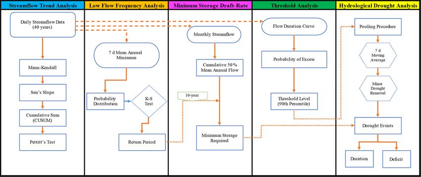
H. H. Hasan et al.: Assessment of probability distributions and the minimum storage draft rate 5
Figure 2. Summary of the methodological framework.
average annual streamflow were determined after the trend
√ S−1 (S > 0) slope had been verified, using the equation employed by
VAR(S)
Petrow and Merz (2009) to calculate the amount of change
Z= 0 (S = 0) . (2) in the data series by Eq. (5):
√ S−1 (S < 0)
VAR(S)
Xend − Xfirst
The null hypothesis of no trend is rejected if Z>2.575 1XR = , (5)
Xmean
at 99 % significance. In the test statistic, S calculates the
sum of the difference between data points and the associa- where 1XR is the amount of change observed in the data se-
tions between samples to show the presence or absence of ries, Xend is the last piece of the trend slope data, Xfirst is the
a trend. When the value of Z is positive, it gives a posi- first piece of the trend slope data and Xmean is the mean of
tive trend, and it gives a negative trend when Z is a negative all pieces of the slope. The distribution-free CUSUM test is a
value. In this study, the level of significance of 0.05 or 95 % cumulative total of time series deviations of target value and
(p value = 0.05) was used. If their p value was equal to or is capable of detecting abnormal trends, is simple and pro-
less than 0.05 (p value ≤ 0.05), the trend test is considered duces a better graphical representation of results (Sonali and
significant, as shown by Eq. (3) (Coch and Mediero, 2016): Nagesh Kumar, 2013). Let us consider x samples, each of n
size with mean µ0 and standard deviation σ . Then, the cu-
+ (Z > 0)
mulative sum of deviation (Si ) from the target value (mean)
Trend = 0 (Z = 0) . (3)
was calculated using Eq. (6):
− (Z < 0)
Xi
Then, a linear trend analysis was also conducted, and the Si = (xj − µ0 ), (6)
j =1
trend magnitude was determined using the Sen’s slope
method. Sen’s slope is a non-parametric method for deter- where xj is the mean of the j th sample. Finally, by consid-
mining any trend’s slope. It utilizes data from a time series ering a sequence of random variables x1 , x2 , . . . , xT which
that is similarly distributed. The difference in slope was cal- may have a change point at N if xt for t = 1, 2, . . . , N has
culated per changed time for each data point. If a trend is a common distribution function F1 (x), the Pettitt test index
identified in a time series, the slope can be determined using (U ) is defined using Eq. (7) (Ahn and Palmer, 2016):
the slope estimator (β) in the Sen’s slope test. For the entire XT Xn
dataset, the estimator β is the median of all slopes between U= sgn(xj − xi ), (7)
i=1 j =T +1
data points. A positive β indicates an increasing trend, and a
negative β indicates a decreasing trend as given by Eq. (4): where T is the change point, x is the target variable and
yj − yi sgn(xj − xi ) is defined as Eq. (8):
β = Median , (4)
xj − xi
+1, xj > xi
where n is the number of data and i and j are indices with sgn(xj − xi ) = 0, xj = xi . (8)
i = 1, 2, . . . (n − 1) and j = 2, 3, . . . , n. The changes in the
−1, xj < xi
https://doi.org/10.5194/nhess-21-1-2021 Nat. Hazards Earth Syst. Sci., 21, 1–19, 2021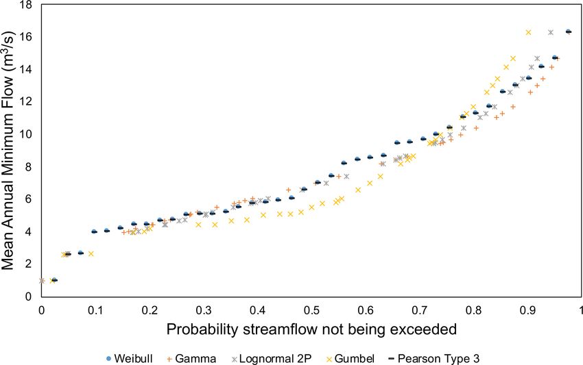
6                         H. H. Hasan et al.: Assessment of probability distributions and the minimum storage draft rate

The non-parametric statistic (Eq. 9) was applied in the eval-      to reject or accept a non-rejected hypothesis, based on the
uation of the change point at which time U has the highest         D value. The graphical illustration of probability plot is de-
absolute value.                                                    scribed as the ith-order statistic of the sample y(i) as a func-
                                                                   tion of a plotting position, which is simply a measure of
K = Maxt ≤T ≤i (U ),                                        (9)    the non-exceedance probability related to the ith-order statis-
where K is the final Pettitt statistic and T is the data point     tic from the assumed standardized distribution (Sharma and
at which the change occurs. The probability of significance        Panu, 2015). The rth-order statistic was acquired by the way
was approximated by p ≈ 2 exp[−6K 2 (i 3 + i 2 )]. When p is       of rating the observed sample from the smallest (i = 1) to the
smaller than the specified significance level (0.05), the null     greatest (i = n) value; then y(i) equals the ith largest value.
hypothesis is rejected.                                            The plotting position of low flow P can be obtained using
                                                                   the Weibull formula (Koteia et al., 2016). The probability se-
3.2   Low-flow frequency analysis                                  lection was made following the shape parameter. This is be-
                                                                   cause it is possible to represent the shape parameter as the
There are many types of frequency distribution functions that      parameter for skewness. For each distribution, Table 2 pro-
have been applied successfully to hydrological data. Fre-          vides the functions of probability density. For this study, the
quency analysis is based on fitting the observed data with         method of maximum likelihood was used for parameter es-
a theoretical probability distribution function and providing      timation. Once the parameters were estimated, the selected
low-flow estimates for any given return period. The choice of      distributions will be tested for the assumption that the ob-
probability distribution is defined as the distribution of prob-   served data is actually from the fitted distribution of prob-
ability with the shape parameter. This selection is necessary      ability. The Kolmogorov–Smirnov (KS) test has been used
to evaluate the shape parameter as the parameter for skew-         to determine the largest discrepancy between the theoreti-
ness. The frequency analysis starts with the calculation of the    cal (Fn (xi )) and empirical (F0 (xi )) cumulative distribution
annual 7 d minimum streamflow series for each gauge station        functions. The KS test obtains a D statistic; if D was higher
in order to determine the suitable probability distribution that   than the critical value (α = 0.05), the distribution was re-
best fits the minimum 7 d low flow in Selangor. Then, four         jected. After the probability calculations P and subsequent
probability distributions, including the gamma distribution,       return periods of the low flow T , the low-flow rate variation
Gumbel, lognormal 2P and Pearson type 3 distribution (PE3)         will be plotted against the return period, with T on the semi-
were evaluated to determine which distribution most appro-         log graph. With this graph, the specific magnitude of a speci-
priately fits the low-flow data. The Kolmogorov–Smirnov            fied period can be determined (Erfen et al., 2015; Gottschalk
(KS) test and ranking method were used to determine the            et al., 2013).
best-fitting distributions. After choosing the optimum prob-
ability distribution, it is important to estimate the values of    3.3   Method for minimum storage draft rate
the variables for certain return periods. The return period of
low-flow occurrence is crucial for determining the magnitude       The water supply or inflow is dependent on low-flow charac-
and frequency of low flow, and such information is useful in       teristics in the stream. If the inflow rate is lower than the out-
minimizing and mitigating the risk of drought in the future.       flow (demand) rate, the cumulative difference between sup-
Four scores ranging from 1 to 4 representing the ranking of        ply and demand volume is the maximum amount of water
distributions in fitting the data were assigned to each station,   drawn from storage during the dry season. In channel stor-
where a score of 1 indicated the best, while a score of 4 in-      age, the function of both outflow and inflow discharge can be
dicated the worst. The summation of scores shows the suit-         considered under two categories as prism and wedge storage.
ability of distribution such that the best distribution got the    The water surface flow in the channel is not only unparallel to
lowest sum of scores. The selected regional probability dis-       channel bottom but also varies with time. The storage, which
tribution function was then used to calculate the annual 7 d       is the maximum cumulative deficiency in any dry season, is
minimum discharge series with a 1-, 2.3-, 5-, 10-, 25-, 50-        obtained from the maximum difference in the ordinate be-
and 100-year return period. The 7 d minimum with a 10-year         tween the mass curve of water supply and demand. Thus, the
return period (7Q10) was used to derive the minimum stor-          storage required can be expressed as per Eq. (10):
age draft rate required for all stations (Sect. 3.3).              S = maximum of (6VD − 6VS ),                                 (10)
   The probabilistic behavior was analyzed using four proba-
bility distribution functions (PDFs), widely used in extreme-      where VD is the demand volume and VS is the supply volume.
value analysis (Joshi and St.-Hilaire, 2013; Zaidman et               The minimum storage draft rate was determined by us-
al., 2003). Then, probability distribution functions were fit-     ing the mass curve of low flow at a monthly interval (Bhar-
ted with their parameters estimated using the method of            ali, 2015). Although specific evaluation of storage require-
maximum-likelihood estimation (Assefa and Moges, 2018).            ments is essential for design, reconnaissance planning can
Goodness of fit was determined by the Kolmogorov–                  frequently be facilitated by using draft storage curves based
Smirnov test. Here, a 95 % confidence level was accepted           on low-flow frequency analysis. Alrayess et al. (2017) de-

Nat. Hazards Earth Syst. Sci., 21, 1–19, 2021                                          https://doi.org/10.5194/nhess-21-1-2021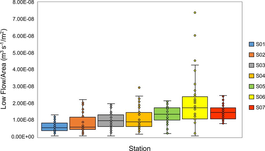
H. H. Hasan et al.: Assessment of probability distributions and the minimum storage draft rate                                             7

Table 2. Probability density function for gamma, Gumbel, lognormal 2P and Pearson type 3 distributions.

                        No.    Distribution      Probability density function                       References
                                                            −α x α−1
                        1      Gamma             f (x) = β 0(α)      exp −xβ                        Baran-Gurgul (2018)
                                                 α>0, β>0, x>0, where α is the loca-
                                                 tion parameter and β is the scale param-
                                                 eter
                                                              h          i
                        2      Gumbel            f (x) = exp exp x−β   α                            Zou et al. (2018)
                                                 −∞0
                                                          β     β−1 −λ(x−ε)
                        4      Pearson type 3    f (x) = λ (x−ε)0(β)e                               Bhatti et al. (2019)
                               (PE3)             x≥ε

termined the capacity of river storage by the mass curve                     3.4        Threshold analysis
method. The mass curve has many useful applications in the
design of storage capacities, such as to determine the storage               An approach based on deficit characteristics under a given
capacity and flood routing (Gao et al., 2017).                               threshold method was adopted to identify extreme low-flow
   The mass curve method can be used to define the storage                   occurrences (Fleig et al., 2006). The low-flow period, which
required for a given draft rate for a monthly record. This ap-               depends on the catchment’s hydrological regime, is defined
proach is limited to draft rates that can be sustained by the                by a fixed threshold level. The selection of the threshold
streamflow available in any single month, that is, by within                 level is influenced by the study, region and available data.
a year of storage. The usefulness of this analysis depends on                The threshold level method can easily obtain the start and
the monthly variability of streamflow. In some regions, the                  the end times of a drought or streamflow deficit period and
maximum draft that can be provided is less than a tenth of                   has been used to define streamflow droughts or deficits. The
the mean flow. In others, notably in Selangor, drafts of half                fixed threshold level in this study is the 90th percentile value
of the mean flow can be provided within a year of storage.                   (Q90 ) of FDC, which was compiled using all the available
The estimation of the storage draft rate in this study will de-              daily streamflow and identified as perennial rivers with river
termine the minimum storage of a river to sustain the water                  flow having continuous flow. The flow duration curve (FDC)
supply during low flows and droughts. The mass curve of                      describes the ratio of a specified percentage of time with dis-
the monthly low-flow rate is used in this analysis to obtain                 charge being equal to or surpassed over a historical period
the minimum storage rate of the river. The procedure for the                 for a particular river basin (Croker et al., 2003; Mohamoud,
mass curve method has the following steps; first, the mass                   2008; Vogel and Fennessey, 1994), which reflects the rela-
curve analysis of low flow for the duration of January to De-                tionship between streamflow magnitude and the length of
cember was plotted against the duration for the recurrence                   time that relates to the average percentage of time of a spe-
interval of 10 years from the 10-year return period in Ta-                   cific flow that had exceeded (Sung and Chung, 2014). The
ble 7. Second, the cumulative draw-off that corresponds to a                 FDC was developed by arranging streamflow values in de-
constant draft rate of 50 % of the mean annual flow and was                  creasing magnitude order and assigning rank numbers to
connected by a straight line. Third, the cumulative draft line               each streamflow value. The most substantial flow was ranked
was superimposed on the mass curve; fourth, the largest in-                  as one, and the smallest flow was ranked as n, where n is the
tercept between the cumulative draft line and the mass curve                 complete record quantity. The percentage of time for a given
was measured. The maximum positive difference between                        flow was equalled or exceeded (probability of excess) when
cumulative draw-off and low flow is the minimum storage                      calculated using the relationship in Eq. (11) (Awass, 2009;
necessary to maintain a draft rate of 50 % of the mean annual                Koteia et al., 2016; Yahiaoui, 2019):
streamflow. The example of minimum storage required in the
river for station S05 using mass curve analysis was shown in                 P = [r/(n + 1)] × 100,                                     (11)
Fig. 3.
                                                                             where P is the percentage of time a given flow is equalled
                                                                             or exceeded, n is the total number of records and r is

https://doi.org/10.5194/nhess-21-1-2021                                                       Nat. Hazards Earth Syst. Sci., 21, 1–19, 2021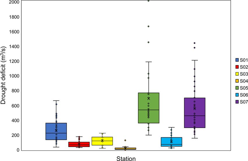
8                         H. H. Hasan et al.: Assessment of probability distributions and the minimum storage draft rate

Figure 3. Minimum storage required using mass curve analysis.

the rank of the flow magnitude. Kannan et al. (2018) in-          4     Results and discussion
dicated the flow duration curve that could be divided into
five zones, representing high flows (0 %–10 %), humid con-        The streamflow data from the seven streamflow gauging sta-
ditions (10 %–40 %), medium-range flows (40 %–60 %), dry          tions will be analyzed in three aspects, which are mean an-
conditions (60 %–90 %) and low flows (90 %–100 %). The            nual low flow and the probability of occurrence, drought
selection of percentile will strongly condition the classifica-   characteristics using the threshold level, and the estimation
tion and evaluation of extreme low-flow events. The magni-        of the storage draft rate of the river. Statistical characteristics
tude of drought characteristics was determined by the thresh-     were calculated from the observed 40-year daily streamflow
old value and the difference in value between the time se-        time series: the mean, minimum and maximum; standard de-
ries. When compared to the use of standardized drought in-        viation; skewness; and kurtosis for each station (Table 3).
dices, a major benefit of this approach is that it allows the
deficit volume to be quantified, which is a critical aspect       4.1    Streamflow trend analysis
in the management of water supplies. When the flow falls
below the threshold level, a drought event begins; it termi-      Annual streamflow series trend analysis presents the over-
nates when the flow exceeds the threshold level. The dura-        all view of the shift in systems of streamflow (Assefa and
tion; total deficit, which is the sum of the deficits; and mag-   Moges, 2018). The Mann–Kendall test, Sen’s slope, rel-
nitude of each drought event can be readily obtained. As the      ative change within 40 years, maximum cumulative sum
daily data series was used, the existence of minor drought        (CUSUM) with the year of change point and their value of
events and mutually dependable drought events can be de-          p using the Pettitt test are displayed in Table 4. In the trend
tected (Van Loon and Van Lanen, 2013). In order to deal           significance test, the significance level of α = 0.05 was set
with this problem, pooling procedures such as moving aver-        as the standard, making Zα/2 = 1.96. The analysis indicated
age, inter-event time criterion and inter-event time, and vol-    that five selected stations (S01, S02, S04, S05 and S07) have
ume criterion were frequently used (Sung and Chung, 2014).        increasing trends of streamflow. Two of the stations, S03 and
According to the study by Sakke et al. (2016a), to eliminate      S06, showed a decreasing trend with the negative change of
the minor drought events, the events that have occurred for       streamflow. The estimation of the trend slope was carried
less than 15 d will be excluded, while the mutually depen-        out using the Sen’s slope estimator, where an upward (down-
dent events were also eliminated using the pooling procedure      ward) streamflow trend is indicated by a trend slope greater
(Sakke et al., 2016b). In this paper, the 15 d of inter-event     (less) than zero. In order to compute the trends of annual
time and 7 d moving average was applied as a pooling pro-         streamflow, the trend slope values were also used to construct
cedure to obtain smooth data. Through these methods, the          a trend line. Using Eq. (5), the amount of change in annual
mutually dependent drought events will combined into indi-        streamflow was determined. The analysis results indicate that
vidual and independent drought events (Fleig et al., 2006).       the amount of change in the basin of station S04 was higher
The minor drought events will be eliminated or combined           than that at other stations (Table 4). The two gauging stations,
with individual drought events automatically (Yahiaoui et al.,    which are S03 and S06, had significantly greater changes that
2009).                                                            showed a downward decreasing trend of −20 % and −55 %,
                                                                  respectively. Streamflow trends indicate variability from one
                                                                  station to another, in terms of magnitude and trend direction.
                                                                  In the S03 and S06 stations, there could be several factors for

Nat. Hazards Earth Syst. Sci., 21, 1–19, 2021                                         https://doi.org/10.5194/nhess-21-1-2021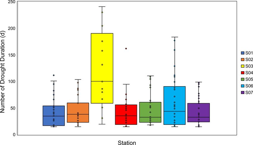
H. H. Hasan et al.: Assessment of probability distributions and the minimum storage draft rate                                         9

Table 3. The statistical analysis for time series of streamflow (1978–2017).

                       Station    Mean flow         Minimum          Maximum      Standard    Skewness    Kurtosis
                       no.         (m3 s−1 )    flow (m3 s−1 )   flow (m3 s−1 )   deviation
                       S01             34.32              1.00           552.62     31.326        4.027     35.819
                       S02             10.23              0.30           153.87      9.595        4.197     32.222
                       S03              5.17              0.15            32.41      3.730        2.296      8.996
                       S04              2.07              0.12            11.93      1.426        1.967      5.726
                       S05             55.12              3.17           272.59     35.083        1.558      3.163
                       S06              8.86              0.14            52.51      5.851        1.491      3.716
                       S07             47.57              8.57           244.75     28.845        1.427      2.744

decreasing streamflow. Some of this involves modifications               by the state government such as the construction of a feeder
in the catchment of physical characteristics such as changes             canal for agricultural and repair of the collapsed stretch of
in land cover in river basins (Hisdal et al., 2001). Another five        the riverbank that caused the widening of the river channel.
stations indicated an increase in trends of streamflow due to               For the mean annual streamflow at the gauging stations,
climate change for the increasing temperature and soil water             five stations indicated an upward trend, and two stations in-
evaporation (Siwar et al., 2013; Taye et al., 2011).                     dicated a downward trend in the 40 years of data. The in-
   The accuracy of the results of data analysis is of crucial im-        terpretations of trend analysis for relatively partial stream-
portance in the trend analysis studies, especially on the dis-           flow records may only reflect a short-term condition and may
charges of any stream. The majority of station trends on the             not be a representative of an actual long-term change in the
main and secondary branches of the basin reflected good con-             streamflow data. This issue is valid for relatively short-term
sistency in this analysis. Two main rivers, however, demon-              records that begin or end in a historically low-flow condi-
strate a paradox, although one station shows a declining trend           tion. From the average annual streamflow results, the change
and the other station shows an increasing trend. Due to the              point is seen to be present at a 100 % confidence interval in
location of the stations, dam construction, linking of another           1996–1997 and 2005–2007 and implies that there is an im-
stream to the channel, irrigation and other disruptions in the           pact of rapidly increasing industrial activities in the basin as
discharge regime of the river, this condition is foreseeable.            well as a change in the pattern of land use induced by the ef-
Stations S01, S02, S03 and S04 are located on the same                   fect of streamflow patterns in the basin which is supported by
stream, but the trends at station S04 are not in the same di-            research according to Abdullah and Nakagoshi (2006). This
rection. Stations S01, S02 and S03 have a significantly in-              study is very useful in interpreting climate change scenar-
creasing trend, while station S04 shows no significant down-             ios and is focused on the revealed characteristics of regional-
ward streamflow trend, caused by the disruption in the river             level hydrological variables.
regime, such as the construction of the Langat dam, which                   The anthropogenic effect is shown by transformations of
may cause this contrast (Memarian et al., 2012).                         water surface such as the construction of reservoirs, a trans-
   The results of the change point in annual streamflow are              basin diversion project, crop irrigation, urban water supply
tabulated in Table 4 using the Pettitt test. For each time se-           or drainage, and urbanization. There are three strategic dams
quence, the result gave the most likely change point event.              in the study area. Those are the Langat dam in S02, the Se-
For the annual streamflow, the results showed that 1997 was              menyih dam in S03 and the Selangor River dam in S05. All
the most probable year of change with a p value of 0.0004.               the dams are functional for domestic and industrial freshwa-
Some stations show signs of a change point at a significance             ter supply. Whereas, the Langat dam is only used as a power
level of 5 %, while the others do not. The prediction of pro-            supply generator for Langat Valley consumption. A study
cess changes and trend generation is well indicated using                by Shaaban and Low (2003) showed that drought events re-
CUSUM charts. This analysis shows a change point that can                duced water discharge at the Langat and Semenyih basin,
be seen in the year of 1996, with a confidence interval set-             particularly in the period of 1993–1998 (Shaaban and Low,
ting of 95 % and the p value of 0.1215 for station S01. The              2003). This event justified the change point from this analy-
change point occurred in 2005 twice for stations S05 and S07             sis. These drought events have decreased the trend of water
in the state of Selangor. The major changes in the annual                discharge in the Semenyih basin. Due to the increasing size
streamflow observed revealed that the presence of rapidly in-            of natural or artificial dams, the reduction of streamflow trend
creasing industrial activities in the basin due to a shift in the        was regulated at the Langat River basin as compared to the
land use is caused by the result of the streamflow trend in the          Semenyih basin.
basin. The latest change points occurred in 2009 at Bernam                  Streamflow variability due to potential human interven-
River (S06) with a new implementation of several projects                tion or climate change is important for regional water supply

https://doi.org/10.5194/nhess-21-1-2021                                               Nat. Hazards Earth Syst. Sci., 21, 1–19, 2021
10 H. H. Hasan et al.: Assessment of probability distributions and the minimum storage draft rate
Table 4. Trend analysis for time series period.
Station Record Mann–Kendall Sen’s slope Relative Maximum Change Value
length change within cumulative point of p
the record (%) sum (year) (Pettitt test)
(CUSUM)
S01 1978–2017 0.03 0.30 36.51 6 1996 0.1215
S02 1978–2017 0.00 0.15 21.80 14 1997 0.0004
S03 1978–2017 −0.46 −0.02 −20.00 8 2006 0.1295
S04 1978–2017 0.03 0.02 43.47 8 2007 0.0845
S05 1978–2017 0.62 0.06 12.05 4 2005 0.4469
S06 1978–2017 −0.35 −0.06 −55.56 8 2009 0.0086
S07 1978–2017 0.14 0.20 39.22 8 2005 0.2286
Note that for the Mann–Kendall test and Sen’s slope, the positive values mean increasing trends and negative ones mean decreasing trends.
planning and management. Knowledge of streamflow vari-
ability and its trend is crucial for the socio-economic sector
because any changing in streamflow is a limiting factor for
the use of water resources. The streamflow decreasing trend
could result in important economic losses and affect health
and human welfare, as well as the aquatic ecosystems. One
of the influential aims of the time series trend is to define the
nature characteristic represented by the sequence of observa-
tions and predicted future values of the time series variable.
The analysis of the observed data for changes and trends of
streamflow data can be used to assess the impact of climate
change. The streamflow trend can estimate future water avail-
ability to maintain and sustain ecosystem functions. More-
over, streamflow trend analysis can also be used to predict Figure 4. Probability of mean annual minimum flow for station S01.
any change in river flows for making water withdrawal deci-
sions, which indirectly could improve drought management
response.
streamflow. Table 6 shows the best-fit results of the KS test
and p-value results with their ranking.
4.2 Low-flow frequency analysis The purpose of the probability distribution fitting is to rep-
resent the low-flow probability most accurately. Among all
Frequency analysis has focused on fitting a theoretical proba- stations, it was found that among all distributions, the log-
bility distribution function to the observed data and provides normal 2P yielded the most cases of best-fit distributions,
low-flow estimates for any given return period. For each sta- while the Gumbel and gamma results yielded the second and
tion, annual minimum streamflow was plotted using all the third most cases of best fits, respectively. Comparatively, it
distributions. The goodness of fit was performed using the is proposed that lognormal 2P distributions predict low-flow
Kolmogorov–Smirnov test. All the PDFs were ranked for discharges for all the rivers under analysis, which can be
streamflow at each station. Ranks, according to these three used in water quality and quantity management at gauged
goodness-of-fit metrics, showed a significant variation. In the and ungauged areas. From this comparison, although a three-
case of annual minimum streamflow, various distributions parameter metric in the probability distribution functions are
were found to be the best fit for different stations, namely, more advantageous, the 7 d low-flow sequences fit better.
gamma, Gumbel, lognormal 2P and Pearson type 3. Fig- However, in the Selangor region, a two-parameter metric is
ure 4 shows the example probability of mean annual min- more suitable, which optimally fits a 7 d mean annual mini-
imum flow for station S01. The estimated parameters were mum flow verified in the studies of Granemann et al. (2018)
determined and shown in Table 5. The information on the and da Silva Lelis et al. (2020). When the best-fit probability
return period of extreme events can be used in determining distribution of the low-flow series of the 7 d has been deter-
the risk management by extreme events such as hydrologi- mined, the low-flow discharge of the 7 d can be estimated ac-
cal drought, while the geographical station location and the cording to any given return period. It should be noted that
surrounding environmental factors determine the variation of the research is station dependent in this analysis. Table 7
Nat. Hazards Earth Syst. Sci., 21, 1–19, 2021 https://doi.org/10.5194/nhess-21-1-2021H. H. Hasan et al.: Assessment of probability distributions and the minimum storage draft rate 11
Table 5. Estimated parameters for the gamma, Gumbel, lognormal 2P and Pearson type 3 distributions.
Distribution Parameters
S01 S02 S03 S04 S05 S06 S07
Gamma α = 4.24 α = 1.92 α = 4.08 α = 3.20 α = 8.13 α = 1.83 α = 9.69
β = 1.78 β = 1.53 β = 0.55 β = 0.24 β = 2.52 β = 2.10 β = 1.60
Gumbel σ = 5.92 σ = 1.92 σ = 1.78 σ = 0.57 σ = 17.17 σ = 2.55 σ = 13.42
µ = 2.89 µ = 1.64 µ = 0.87 µ = 0.33 µ = 5.94 µ = 1.68 µ = 5.47
Lognormal 2P σ = 8.09 σ = 3.10 σ = 2.45 σ = 0.75 σ = 20.65 σ = 3.70 σ = 16.46
µ = 4.81 µ = 2.21 µ = 1.63 µ = 0.42 µ = 7.49 µ = 2.79 µ = 6.92
Pearson type 3 α = 1.07 α = 2.46 α = 2.87 α = 7.78 α = 0.60 α = 2.00 α = 0.63
β = 5.00 β = 5.00 β = 5.00 β = 5.00 β = 5.00 β = 5.00 β = 5.00
Table 6. The values of the Kolmogorov–Smirnov (KS) test.
Station Distribution KS test pvalue Rank
statistics
S01 Gamma 0.09 0.9110 2
Gumbel 0.09 0.8581 3
Lognormal 2P 0.08 0.9626 1
Pearson type 3 0.23 0.0204 4
S02 Gamma 0.09 0.9074 2
Gumbel 0.10 0.8241 4
Lognormal 2P 0.09 0.8823 3
Pearson type 3 0.07 0.9796 1
S03 Gamma 0.09 0.8810 2
Gumbel 0.09 0.8984 1
Lognormal 2P 0.10 0.8275 3
Pearson type 3 0.12 0.5866 4
S04 Gamma 0.10 0.8181 2
Gumbel 0.11 0.7430 3
Lognormal 2P 0.09 0.9004 1
Pearson type 3 0.19 0.0989 4
S05 Gamma 0.08 0.9401 1
Gumbel 0.09 0.8956 3
Lognormal 2P 0.09 0.9062 2
Pearson type 3 0.35 0.0001 4
S06 Gamma 0.12 0.6354 4
Gumbel 0.07 0.9905 1
Lognormal 2P 0.10 0.8296 2
Pearson type 3 0.11 0.7418 3
S07 Gamma 0.10 0.8406 3
Gumbel 0.09 0.8990 2
Lognormal 2P 0.08 0.9608 1
Pearson type 3 0.36 0.0001 4
https://doi.org/10.5194/nhess-21-1-2021 Nat. Hazards Earth Syst. Sci., 21, 1–19, 202112 H. H. Hasan et al.: Assessment of probability distributions and the minimum storage draft rate
Figure 5. Boxplot of low flow per watershed catchment area.
shows the return period of low flow at all streamflow stations.
The 7 d mean annual minimum for the recurrence interval of
10 years (Table 7) was used in the determination of minimum
storage draft rate for each station.
A catchment with a slow or quick response to rainfall in-
tensity that usually has prolonged or rapid recession actions
depends entirely on the catchment’s physical characteristics.
Low flow in catchments that respond quickly is lower than
in those that respond slowly. Low flow in catchments that
respond slowly is more persistent than in catchments that
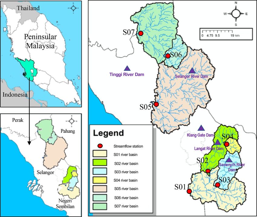
respond quickly. These differences demonstrate the signifi- Figure 6. Minimum storage draft rate with a cumulative 50 % mean
cant effect of hydrological processes and storages to the low- flow at (a) S01, (b) S02, (c) S03, (d) S04, (e) S05, (f) S06 and (g)
S07.
flow events. Figure 5 displays the low-flow relationship with
the watershed area represented by the boxplot graph. The
largest range for low flow per area is in S06, while the small-
est range is in S01. The boxplot graph provides information The minimum storage required for maintaining a draft
about the shape of a dataset. S01, S02 and S04 are skewed rate required for S01 is 21.51 m3 s−1 in October; S02
right; S03, S05 and S06 are symmetrically shaped data; and is 13.37 m3 s−1 in December; and S03 is 4.79 m3 s−1
S07 is skewed left. From the discussions above, it is clear in December. The minimum storage required for S04 is
that the natural elements that affect a variety of factors of the 2.32 m3 s−1 in October for a 40-year duration period, and
river’s low-flow regime consist of distribution and hydraulic S05 is 15.00 m3 s−1 in September. The minimum storage re-
components, climate and topography. quired to maintain the draft rate for S06 is 10.90 m3 s−1 in
October, and lastly, for S07 it is 6.17 m3 s−1 in September.
4.3 Estimation of the minimum storage draft rate The result shows that the water storage for all stations did not
meet the corresponding water required, while stations S05
This study focused on the minimum surface water storage and S07 correspond to the required expectation for August to
required based on the records from the hydrological stations October. This result reveals that the period of September to
in the state of Selangor for the 1978 to 2017 period. Hydro- December is a critical duration in river water storage to sus-
logical drought is a recurring phenomenon of water short- tain the water availability during low flow in a 10-year oc-
age that incorporates the storage of surface and subsurface currence interval. This finding is justified by the state of Se-
water under the effects of climate change and human activ- langor located on the western coast of Peninsular Malaysia
ity (Schwalm et al., 2017). The water storage required for which is affected by two main monsoon seasons and two
all stations is based on their respective monthly streamflow inter-monsoon seasons with October and January being rela-
discharge. A graph of the cumulative streamflow draft rate tively dry months (Hazir et al., 2020). However, there is not
versus a specific historical timeline is plotted to find out the enough water storage starting September for stations S05 and
storage required for each station. Figure 6 shows the mass S07.
curve analysis for the determination of the minimum stor- Low-flow and surface water storage assessment is a crit-
age draft rate of each station that needs to be maintained at a ical issue for understanding the global water cycle, which
draft rate of 50 % of the mean annual flow during low flows is recognized to be of significant importance on a regional
to sustain the water supply. and global scale for the monitoring of water resources. Cor-
Nat. Hazards Earth Syst. Sci., 21, 1–19, 2021 https://doi.org/10.5194/nhess-21-1-2021H. H. Hasan et al.: Assessment of probability distributions and the minimum storage draft rate 13
Table 7. The return period of low flow at all streamflow stations.
Station no. Low flow at return period (m3 s−1 )
1-year 2.3-year 5-year 10-year 25-year 50-year 100-year
S01 21.42 18.19 15.27 12.63 9.13 6.49 3.85
S02 10.60 8.83 7.24 5.80 3.89 2.44 1.00
S03 6.44 5.45 4.55 3.73 2.66 1.84 1.02
S04 2.25 1.90 1.58 1.29 0.91 0.62 0.34
S05 48.40 41.54 35.35 29.72 22.29 16.67 11.05
S06 13.09 10.91 8.93 7.14 4.78 2.98 1.19
S07 34.56 30.14 26.15 22.53 17.74 14.12 10.49
Note that the 10-year low-flow return period will be used in the determination of the minimum storage draft rate.
respondingly, this analysis provides important scientific data
on the minimum storage required for river systems. Sufficient
water storage during critical dry periods is largely dependent
on the adequacy and efficiency of water supplies from sur-
face water resources. This surface water storage faces many
challenges which could lead to a decrease in their optimum
yields and eventually result in inadequate supply of water
over the next 10 years. This could be due to reasons such as
increasing water demand due to increasing population and
industry needs and emerging demands for recreation and the
conservation of the quality of stream water, biodiversity and
aquatic ecosystems.
Figure 7. Number of drought events.
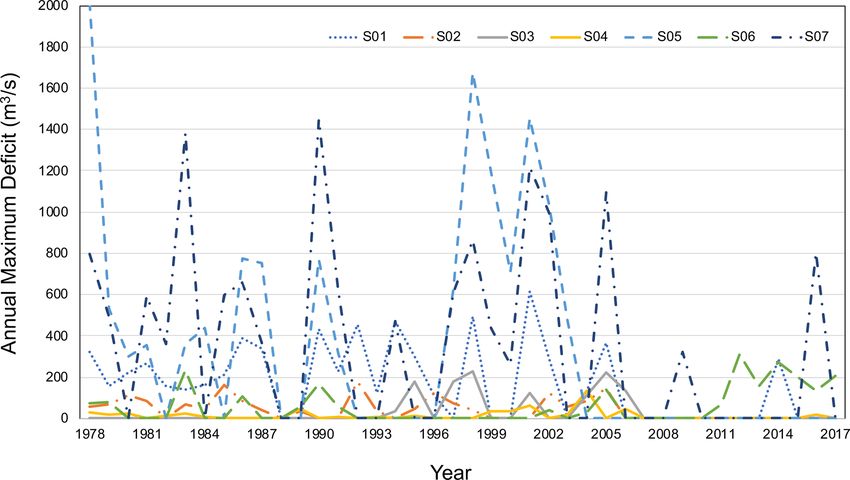
4.4 Hydrological-drought characteristic analysis
The threshold level value per the Q percentile obtained from
the flow duration curve is shown in Table 8. In this study, only
Q90 was used as a threshold level in the determination of
drought events. The percentage is shown where the stream-
flow rate was below the average level, and the respective days
were recorded to show the severity of droughts events at each
station. The growing perception of hydrological-drought im-
provement on a global scale has some necessary implications
for water management. It is recognized, for example, that the
duration and the volume of the deficit of the drought are as-
sociated (Fleig et al., 2006). Figures 7 to 10 show the drought
characteristics below the threshold level (Q90 ), with the mi-
nor drought for each station in the Selangor region removed. Figure 8. Length of drought duration (days).
Station S01 has 39 episodes of drought events in 40 years.
This station also recorded 1593 d of drought, with a total
deficit of 10 299.97 m3 s−1 . The lowest deficit was recorded
in 1994 at 41.53 m3 s−1 , while the highest deficit was drought events in 40 years. The total duration of the drought
recorded in 1986 at 666.58 m3 s−1 . The average amount of events was recorded to be 1261 d from the 14 610 d of total
water deficit was 264.10 m3 s−1 . This river has been affected observation, which was only 8.63 % of the entire record pe-
by water rationing that happened in Selangor in early 2014 riod and was below the threshold level Q90 = 2.99 m3 s−1 .
for 3 to 4 months. The most prolonged period of an individual The overall deficit for this station was 2340 m3 s−1 , with an
drought was recorded in 2014 at 112 d from 5 March to 24 average of 80.70 m3 s−1 . The lowest deficit was in 1993 at
June. The shortest period of a single drought was 15 d, which 34.44 m3 s−1 , while the highest deficit was recorded in 1986
was marked three times in 2004 and 2005. Station S02 was with 179.73 m3 s−1 . The overall total deficit was 1.57 % of
a part of the Langat River basin and has had 29 episodes of the total water flow.
https://doi.org/10.5194/nhess-21-1-2021 Nat. Hazards Earth Syst. Sci., 21, 1–19, 2021You can also read