Robust Adaptation Decision-Making Under Uncertainty: Real Options Analysis for water storage - Deep ...

Robust Adaptation Decision-Making Under Uncertainty:
Real Options Analysis for water storage

 Anita Wreford Lincoln University
 Ruth Dittrich University of Portland
 Christian Zammit NIWA
 Channa Rajanayaka NIWA
 Alan Renwick Lincoln University
 Daniel Collins NIWA

Deep South National Science Challenge
Final Research Report, July 2020

Robust adaptation decision-making under uncertainty: Real Options
 Title
 Analysis for water storage
 Anita Wreford
 Ruth Dittrich
 Christian Zammit
 Author(s)
 Channa Rajanayaka
 Alan Renwick
 Daniel Collins

Author Contact Details
Anita Wreford
Lincoln University
Anita.wreford@lincoln.ac.nz

Acknowledgements
We acknowledge the funding received from the Deep South National Science Challenge, and
the time spent with individuals from ECan, and reservoir engineers and contractors to develop
our understanding of water storage in Canterbury.

We acknowledge feedback on a draft version from Professor Paul Dalziel at Lincoln University,
however none of these organisations are responsible for the information in this paper. Every
effort has been made to ensure the soundness and accuracy of the opinions and information
expressed in this report. While we consider statements in the report are correct, no liability is
accepted for any incorrect statement or information.

Recommended citation
Wreford, A., Dittrich, R., Zammit, C., Rajanayaka, C., Renwick, A., Collins, D (2020) Robust
adaptation decision-making under uncertainty: Real Options Analysis for water storage.
Wellington, Deep South National Science Challenge CO1X112.

© 2020 the authors. Short extracts, not exceeding two paragraphs, may be quoted provided
clear attribution is given. Final research reports are research materials circulated by their
authors for purposes of information and discussion. They have not necessarily undergone
formal peer review.

Deep South National Science Challenge
www.deepsouthchallenge.co.nz

DEEP SOUTH CHALLENGE: CHANGING WITH OUR CLIMATE |3

Contents

Contents ........................................................................................................................................ 4
Executive Summary ....................................................................................................................... 6
1. Introduction .......................................................................................................................... 7
2. Background and literature review......................................................................................... 8
3. New Zealand climate projections and uncertainty ............................................................. 10
 3.1. Simplifying complexity ................................................................................................ 13
 3.2. Hydrological uncertainties due to Global Climate Model uncertainty ....................... 14
4. The case study used in this project ..................................................................................... 16
5. Data and Methods............................................................................................................... 20
 5.1. Climate modelling ....................................................................................................... 20
 Representative Concentration Pathway ............................................................................. 21
 5.2. Hydrological modelling................................................................................................ 23
 5.3. Water demand, water availability and reliability of supply ........................................ 26
 5.3.1 Water demand and availability .................................................................................. 26
 5.3.2 Reliability of supply and reservoir sizing .................................................................... 26
 5.4. The ROA....................................................................................................................... 27
6. Results ................................................................................................................................. 33
7. Discussion ............................................................................................................................ 37
 7.1. Limitations and further work ...................................................................................... 38
8. Conclusion ........................................................................................................................... 42
References................................................................................................................................... 44

DEEP SOUTH CHALLENGE: CHANGING WITH OUR CLIMATE |4

DEEP SOUTH CHALLENGE: CHANGING WITH OUR CLIMATE |5

Executive Summary
Planning for climate change adaptation is challenging due to the inherent uncertainty associated
with future climate changes. Although we have a range of climate projections, even these cannot
provide a definitive picture of the future, with little certainty regarding the timing, magnitude and
location of change. As a result there is increasing interest in approaches that can accommodate
uncertainty better. A range of approaches exist and are being developed across several disciplines.
Each has advantages and disadvantages and is suited for different types of decisions.
In this study we focus on one of these approaches, Real Options Analysis (ROA), and chose water
storage for irrigation as an example to demonstrate its use in uncertain futures.
ROA is most suited to large, one-off investment decisions, such as water storage. Reservoirs are a
significant investment, and without fully considering the range of future water availability, may turn
out to be either too large, or not economically viable. Conversely, without their existence to smooth
out water variability, significant production losses may be experienced in the future.
While we use a case study location in Canterbury, the intention with this analysis is to demonstrate
the process of ROA, the type of information developed, and how it can be used to support decision-
making under uncertainty. The approach can be applied to any type of large irreversible investment
decision.
Using the full range of climate model and warming scenario combinations available in New Zealand
(24), we develop estimates of water requirements out to 2090 for the chosen location. We specify
two decision points: 2018 and 2050, and construct a decision tree with 256 potential paths. We
develop a method to use the range of 26 GCM/RCP combinations available in New Zealand to
generate estimates of likelihood. Using a backward induction technique, we identify the most cost-
effective storage size. In this particular example, the most cost-effective option was to construct a
reservoir for the most conservative climate change outcome in 2018, and in 2050. The decision to
build for the smallest climate change is sensitive to a number of factors however, particularly the
discount rate and the milk price, both of which result in larger reservoirs being more cost-effective in
the first time period. The decision is also sensitive to assumptions regarding the likelihood of future
climate changes – when the higher and lower climate scenarios are assigned a lower likelihood, this
changes the decision to a larger storage size in 2018. This analysis illustrates the benefits of ROA
when the future is uncertain – by enabling decision-makers to adjust their decisions over time
rather than locking themselves into a decision made now that has long-term consequences.
We used an example of water storage on a dairy farm to illustrate how ROA can be used, using the
climate data available in New Zealand. This method is suitable for application across a range of
investment decisions in New Zealand, where the initial cost is large and the investment is at least
partially irreversible. We believe that using ROA for these types of decisions will enable more cost-
effective investment than cost-benefit analysis or other methods that use only a single climate
scenario.

DEEP SOUTH CHALLENGE: CHANGING WITH OUR CLIMATE |6

1. Introduction
Planning for climate change adaptation is challenging due to the inherent uncertainty associated
with future climate changes. Although we have a range of climate projections, even these cannot
provide a definitive picture of the future, with little certainty regarding the timing, magnitude, and
locations of change. Within climate models and their projections, a wide range of futures exist,
creating uncertainty for decision-makers. This uncertainty stems from four main sources:
 • Scenario uncertainty due to different concentrations of greenhouse gases (GHGs) in the
 atmosphere. This depends on how successful the global community is at reducing emissions;
 • Response uncertainty due to limitations in understanding of climate processes and how they
 are represented in climate models;
 • Uncertainty in natural climate variability;
 • Uncertainty in downscaling emissions (CSIRO and BOM 2015)
Despite this uncertainty, many adaptation decisions need to be made now, in advance of climate
change, to effectively reduce future vulnerability to climate change. Nonetheless, it is clear that
uncertainty creates challenges. Decisions with long-term implications, such as investment in capital,
risk locking decision-makers into a certain path with little flexibility to change if other conditions,
such as the climate, change.
Because of the challenge of uncertainty, there is increasing interest in approaches that can
accommodate uncertainty better. We present further background and briefly review these
approaches in the next section. In this project, we focus on one of these approaches, Real Options
Analysis (ROA), and chose water storage for irrigation as an example to demonstrate its use in
uncertain futures.
ROA is most suited to large, one-off investment decisions. Constructing a water storage reservoir, or
dam, is an appropriate example, and particularly pertinent in New Zealand where there is increasing
interest in, and construction of these. These reservoirs are a significant investment however, and
without fully considering the range of future water availability, may turn out to be either too large,
or not economically viable. Conversely, without their existence to smooth out water variability,
significant production losses may be experienced in the future.
We use a case study location in Canterbury, but the intention with this analysis is to demonstrate
the process of ROA, the type of information developed, and how it can be used to support decision-
making under uncertainty. The report is structured as follows: In the following section (section 2)
we provide a background to decision-making under uncertainty, and a literature review of the
approach taken for this study, ROA. Section 3 provides a summary of climate projections for New
Zealand and an overview of uncertainty in this context. Section 4 outlines the case study used to
demonstrate the ROA method in this study, and section 5 presents the data and methods used.
Section 6 presents the results, while section 7 discusses their implications and limitations, and
section 8 concludes.

DEEP SOUTH CHALLENGE: CHANGING WITH OUR CLIMATE |7

2. Background and literature review
There is increasing interest in decision-making under uncertainty, as it becomes apparent that
planning for future climate changes needs to begin now, despite the inherent uncertainty in
understanding the details of the timing, magnitude and location of the climate impacts.
Decision-making under uncertainty (DMUU) is emerging as a body of approaches, using both
economic and other techniques, to handle uncertainty. DMUU uses principles such as robustness,
flexibility, learning and diversification, to address the challenge of uncertainty in the design of
practical adaptation plans and projects. In the area of adaptation economics, support methods and
tools for the economic appraisal of adaptation are increasing (Dittrich et al. 2016, Watkiss et al.
2015). Complementary approaches outside of economics include adaptive management, iterative
risk management (IPCC, 2014), adaptation pathways (Downing, 2012), and dynamic adaptation
pathways (Haasnoot et al. 2013).
Alternative decision-making approaches to appraise and select adaptation options are being
explored, both in the academic and policy literature (Dessai & van der Sluijs, 2007; Hallegattee al.
2012; Ranger et al., 2010). The aim is to better incorporate uncertainty while still delivering
adaptation goals, by selecting projects that meet their purpose across a variety of plausible futures
(Hallegatte et al., 2012); so-called ‘robust’ decision-making approaches. These are designed to be
less sensitive to uncertainty about the future and are thus particularly suited for deep uncertainty
(Lempert & Schlesinger, 2000). Instead of optimising for one specific scenario, optimisation is
obtained across scenarios: robust approaches do not assume a single climate change projection, but
integrate a wide range of climate scenarios through different mechanisms to capture as much of the
uncertainty on future climates as possible. This is achieved in different ways: Portfolio Analysis (PA),
for example, reduces the risk of choosing a single adaptation option that may prove inappropriate by
combining several adaptation options in a portfolio. It is thus akin to combining different stock
market shares in a portfolio to reduce risk by diversification (Markowitz, 1952). Real Options Analysis
(ROA) develops strategies that can be adjusted (e.g. up-scaled or extended) when additional climate
information becomes available. It handles uncertainty by allowing for learning about climate change
over time and originates from option trading in financial economics (Merton, 1973, Cox et al., 2002,
Wreford et al. 2020). Finally, Robust Decision Making (RDM) identifies how different strategies
trade-off in order to identify options which might not be optimal under a specific climate outcome
but rather less vulnerable under many climate outcomes. These techniques are particularly suited
for adaptation options with long lead and/or life-times as they integrate uncertainty in the decision-
making process. For a more detailed overview of robust approaches, see Dittrich et al. (2016) and
Watkiss et al. (2015).
Real Options Analysis is the extension of the option pricing theory for managing real assets. The
financial option valuation tool was systematically developed by Merton in his article “The theory of
rational option pricing” (Merton, 1973) building on Black and Scholes’s (1972) theory of valuation of
contingency claims. Following from there, the model evolved in several branches, summarised
below. Designers of military equipment also use a similar concept, where equipment may be fitted
“for but not with” the capability of being equipped in future with missiles (Dobes, 2010). ROA is

DEEP SOUTH CHALLENGE: CHANGING WITH OUR CLIMATE |8

different from traditional financial tools, which generally provide a fixed path for future investment
decisions. In ROA, options are left open in the future, assuming a gradual resolution of uncertainty,
making it ideal for assessing large-scale investments in the context of climate change. The solution
of real options models is based on different techniques, such as the Black-Scholes formula, Monte-
Carlo path dependent simulations and binomial or multinomial trees (Kontogianni et al. 2014).
The learning in ROA is based on an uncertain underlying parameter. The uncertain parameters in the
context of this project will be rainfall and river and aquifer flows. Due to climate change (and
changes in land use and river basins), hydrological variables will no longer be reliably constant and
past hydrologic data do not necessarily provide a good indicator of future conditions, i.e. non-
stationarity applies (Milly et al., 2008). In ROA, the uncertainty of the hydrological variable - at least
with respect to climate change - is assumed to resolve with the passage of time due to increasing
knowledge. For instance, the confidence in changes of rainfall, extremes and related drought risk
under climate change will likely increase over time as time series grow longer, as ‘low-data’ methods
are developed and as model uncertainties in climate and hydrological models are reduced (van der
Pol et al. 2014). ROA takes advantage of the assumption that the uncertainty is dynamic rather than
deep and provides strategies that can be adapted in a changing context.
The ROA method selected depends on the available data, the type of option and the desired
simplicity (Kontogianni et al., 2014). In this study we choose the multinomial tree method.
The majority of ROA studies in the adaptation context apply ROA to an aspect of flood risk
management, including coastal sea-level rise. The dominance of studies around flooding reflects the
usually high irreversible fixed cost that makes waiting attractive, and the coastal application lends
itself to ROA because it involves a uni-directional, bounded and gradual change. Many studies (e.g.
Abadie et al., 2017, Rosbjerg, 2016) use the approach to determine whether it is optimal to invest
now or to delay the investment, while others (Woodward et al., 2014, 2011, Gersonius et al. 2013)
use ROA to determine the value of flexibility within the system, as well as the difference in value
between waiting and investing now. These two approaches are sometimes referred to as “on”
options, which have a timeliness aspect, and “in” options, which have technical engineering and
design adjustments enabling options within operations.
Some studies do apply ROA to water storage, either for hydropower (Kim et al., 2017, Steinschneider
& Brown, 2012) or reservoirs for other uses (Sturm et al., 2017). Again the analysis is either on or in
options: Kim et al. (2017a) apply ‘in’ options to look at the optimal sequential expansion of rainwater
harvesting tanks.
Kim et al. (2017b) assess the economic benefit of adapting hydropower plants to climate change in
South Korea. They assess whether to build a hydropower plant under either RCP 4.5 or RCP 8.5, with
no uncertainty considered within each RCP. The climate change risk is in the form of the quantity
and timing of runoff and extreme weather events, including floods and droughts. They use a similar
approach as Gersonius et al. (2013) to determine the probability, and for the volatility, a ratio of
best/worst case. The best case is created assuming that the energy production and tariff increase to
maximum, whereas investment and operating and maintenance costs decrease to minimum
compared with those of the moderate case. The findings indicate that under RCP 8.5 the investment
should not go ahead, as the investment cost exceeds the economic payoff.
DEEP SOUTH CHALLENGE: CHANGING WITH OUR CLIMATE |9

Steinschneider and Brown (2012) apply ROA to compare different adaptation strategies for a
hydropower facility in the US under a range of possible future climates. The utility of these
adaptation strategies are tested with and without the availability of a real option water transfer. The
first strategy assumes stationary climate conditions will persist into the future and conditions
reservoir operations on the historic record. The second strategy optimises operations for the mean
projections of future climate as simulated by the GCMs. The third strategy dynamically manages the
system for short term climate variability using seasonal hydrologic forecasts. For the third strategy,
the authors suggest using seasonal hydrologic forecasts in combination with ROA-style hedging
rather than trying to use long-term projections which are highly uncertain. The real option is the
possibility to transfer water between the water supply agency and a nearby flood control reservoir
that is established to augment supply in times when water is over-allocated and shortages are
imminent.
The study indicates that seasonal hydrologic forecasts are a promising adaptation to nonstationary
hydrology, even without the support of a risk hedging option. Surprisingly, the option approach
enabled even a stationary assumption to perform well in the future, suggesting that option
instruments alone can act as a robust adaptation mechanism.
Sturm et al. (2017) apply ROA options to compare the prices of water storage and no water storage.
They use an option pricing approach, i.e a simplified Black-Scholes formula to evaluate strategic
decisions, applying it to two examples, one of which is water storage. They replace the finance
variables in the formula with climate variables, using the example of the development of water
storage through a system of rivers, dams and reservoirs for California, and compare the option price
of storage and no storage ad examine the difference.
The purpose of applying ROA in the context of climate change is to assist in making decisions when
there is uncertainty involved. ROA assumes that the uncertainty is dynamic rather than deep and
while it will not completely resolve over time, the probability distribution will be adjusted in future
as time series of data grow longer, ‘low-data’ methods are developed and model uncertainties in
climate and hydrological models are reduced. This agreement on probabilities does mean the
technique is vulnerable to bias, gridlock and brittle decisions (Kalra et al., 2014), but still provides
advantages over traditional non-flexible approaches.
Some large-scale modelling assessments have developed probability-like projections, notably the
UKCP09 projections (Murphy et al., 2009), however these only sample climate model uncertainty
(i.e. a probability distribution function (pdf) for each separate emission scenario), rather than a
single pdf of the overall envelope of difference scenarios and all climate models together. In this
study we develop an approach to assign probabilities to a range of climate model and climate
scenario combinations.

3. New Zealand climate projections and uncertainty
Climate change is already affecting New Zealand with downstream effects on the natural
environment, the economy, and communities. In the coming decades, climate change is highly likely
to increasingly pose challenges to New Zealanders’ way of life.
DEEP SOUTH CHALLENGE: CHANGING WITH OUR CLIMATE | 10

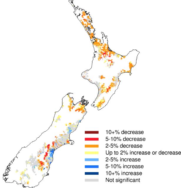
In general, New Zealand can expect ongoing warming throughout the 21st century, as well as
changes to extreme temperatures. Extreme warm temperatures and heatwaves are likely to be
more common in the future, and extreme cold temperatures and frosts are likely to decrease. In
addition, rainfall patterns may change across the country, with the west and south of New Zealand
becoming wetter and the north and east of the North Island becoming drier. Some areas may not
experience much change in total annual rainfall, but the seasonality when rainfall occurs may
change, i.e. summers may become drier and winters may become wetter (Figure 1). The intensity of
extreme rainfall is likely to increase in a warmer climate. Winds are also likely to increase across

DEEP SOUTH CHALLENGE: CHANGING WITH OUR CLIMATE | 11

central New Zealand, particularly in winter.

Figure 1 : Annual mean rainfall change (in %) between 1995 and 2090, under the highest IPCC
Representative Concentration Pathway (RCP8.5).

These changes are likely to have significant impacts on the country’s water cycle. This in turn will
affect the availability of water for irrigation and crop demand for irrigation, and as such affect New
Zealand’s agricultural systems.

DEEP SOUTH CHALLENGE: CHANGING WITH OUR CLIMATE | 12

Increasing temperatures will impact pasture grass and crop growth, as plant phenological
development may occur at a faster rate. The pasture growth season may extend into the cooler part
of the year as the climate warms, and higher concentrations of carbon dioxide in the atmosphere
means that pasture may grow more vigorously when it is not constrained by temperature or water
availability.
Extreme heat affects the rate of evapotranspiration, or the uptake of water by plants. Therefore,
increases to extreme heat may affect water availability and increase the amount of water needed for
irrigation, as under hot conditions plants use more water than usual. Extreme heat may also result in
current varieties of crops and pasture becoming unsustainable if they are not suited to growing in
hot conditions.
Reductions in cold conditions may have positive impacts for diversification of new crop and grass
varieties that are not able to currently be grown in cooler parts of New Zealand. However, future
warmer temperatures may increase the risk from pests (plants and animals) and diseases. Currently,
many pests are limited by New Zealand’s relatively cool conditions, so that they cannot survive low
winter temperatures, and therefore their spread is limited (Kean et al., 2015). Under a warmer
climate, these pests may not be limited by cold conditions and therefore cause a larger problem for
farmers and growers in New Zealand.
Increases in extreme rainfall event magnitudes may impact agriculture and horticulture in several
different ways. Slips on hill country land may become more prevalent during these events, and soil
erosion may also be exacerbated by increasing drought conditions followed by heavy rainfall events
(Basher et al., 2012). This has impacts on the quality of soil, the area of land available for production,
and other impacts such as sedimentation of waterways (which can impact flooding and water
quality). Slips may also impact transport infrastructure (e.g. roads, farm tracks) which may in turn
affect connectivity of farms and orchards to markets.

 3.1. Simplifying complexity
A degree of simplification, aiming at reducing the complexity of the results, is necessary to convey
and frame the science appropriately for diverse audiences. Those simplifications can be achieved in
a number of ways such as: i) conveying the effects in summary qualitative terms rather than
quantitative; ii) confining the suite of dependent variables reported; ii) choosing to convey spatial or
temporal averages of summary statistics (e.g. minimum flows to support water allocation process);
iii) selecting only a subset of GCMs (e.g. choosing GCM that better represent historical observation);
iv) defining a limited set of scenarios to serve as RCPs (e.g. planning for the worst case scenario); v)
selecting only a subset of defined scenarios/RCPs; vi) averaging results across the GCMs; or vii)
combing results across RCPs by treating RCPs probabilistically rather than separately
Of the simplifications listed above, the most challenging is where RCPs are probabilistically combined
to represent end-user perception of future emission scenario. RCPs were defined to represent
plausible and distinct scenarios along a continuum of multi-dimensional possibilities, helping to
clarify how the climate may be driven in the future. They are based on a number of assumptions and
simplifications about how society will behave and what technologies will become available. They

DEEP SOUTH CHALLENGE: CHANGING WITH OUR CLIMATE | 13

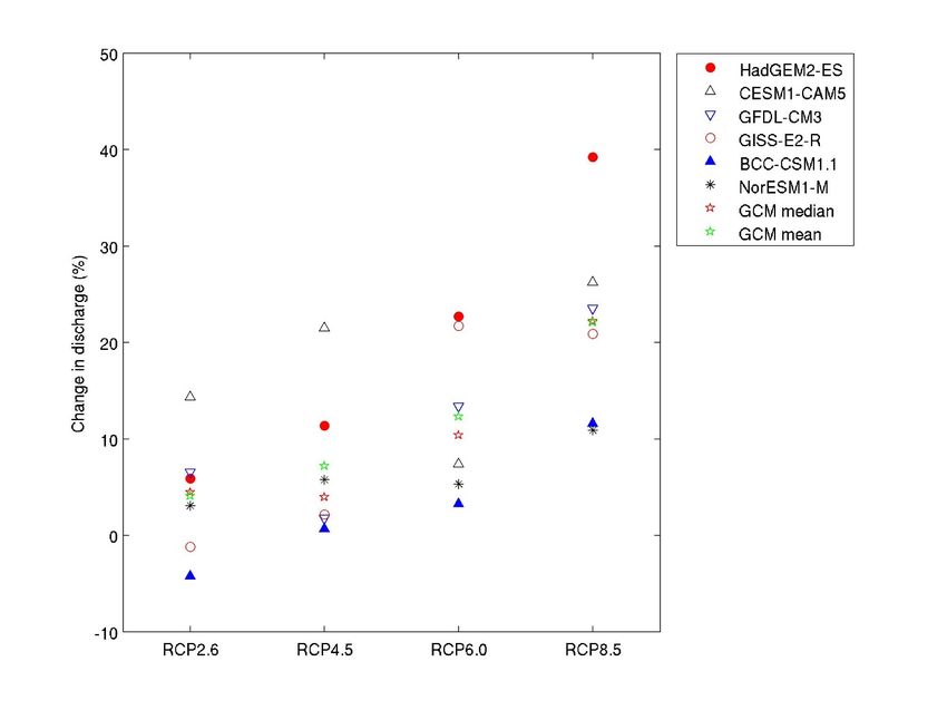
help to highlight implications of climate change mitigation, but are currently a source of uncertainty
and complexity to guide adaptation decision making.
Despite the substantial knowledge encapsulated by the modelling chain used to generate models
and datasets, due to their nature errors and uncertainties remain and can influence interpretation
and analysis results. Uncertainties related to climate change fields are discussed in detail in Ministry
for the Environment (2018).

 3.2. Hydrological uncertainties due to Global Climate Model
 uncertainty
Multiple GCMs are used in order to encapsulate a plausible range of physical interpretations of the
climate system given uncertainties in climate science. The IPCC assessment contains an ensemble of
more than 41 GCMs. NIWA selected 41 to be used in New Zealand, but the number of simulations
available varied with RCP – only 23 for RCP2.6, but the full 41 for RCP8.5 and this historical period
ending 2005. Thus among those GCMs, a subset of 23 GCMS was established to be used in New
Zealand for the four RCPs (Ministry for the Environment 2016). A further subset of six GCMs to be
used for dynamical downscaling was established representing the wide range of potential climate
condition across New Zealand for each RCP (Ministry for the Environment, 2018). Each GCM will
invariably produce a unique and different hydrological outcome. To illustrate the potential variability
of these outcomes,

DEEP SOUTH CHALLENGE: CHANGING WITH OUR CLIMATE | 14

Figure 2 illustrates the variation across GCMs and RCPs for the change in mean discharge in the
Waikato river for each individual GCM and RCP as well as the mean and median of GCM results. For
the lower three RCPs, the variation among GCMs is greater than the variability among RCPs.
Differences in the distribution of the GCM results for a given RCP also affect the relative position of
the GCM mean and median: while the GCM mean increases monotonically across RCPs, the GCM
median does not.
The GCM hindcasts are also biased to a degree. This is addressed through the bias correction and
downscaling described by Sood (2014).

DEEP SOUTH CHALLENGE: CHANGING WITH OUR CLIMATE | 15

Figure 2: Change in mean discharge by end of the century at the outlet of the Waikato River for individual
GCMs and RCPs, including GCM means and medians.

4. The case study used in this project
In this study, we focus on the uncertainty relating to future water availability for agriculture in New
Zealand. Water availability for irrigation, industry and domestic use is currently under considerable
pressure in NZ, and is likely to increase further with extreme events (droughts) and increased rainfall
variability under climate change, combined with ever-increasing demand. Increasing requirements
to leave more water in lowland stream and aquifers for environmental values (Ministry for the
Environment and Ministry for Primary Industries 2018) means that new thinking is required to bring
reliability of supply to acceptable levels. Water storage is a potential adaptive measure, harnessing
rainfall and water fluxes in periods of excess for use when less is available, and improving the
reliability of supply. Storage facilities are a significant investment however, and standard decision-
making approaches (such as cost-benefit analysis), using a specified climate change scenario in order
to identify a single optimal adaptive strategy, may lead to sub-optimal decisions.

DEEP SOUTH CHALLENGE: CHANGING WITH OUR CLIMATE | 16

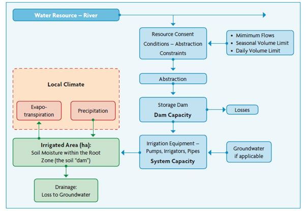
Dittrich et al. (2016) provide advice on the choice of robust approach in different contexts, and
recommend that ROA is most appropriate for large capital infrastructure investments. ROA is suited
for (partly) irreversible investments with long life-times and sensitivity to climate conditions when
there is a significant chance of over- or underinvesting combined with an opportunity cost to
waiting, i.e. if there is a need for action in the present. We will therefore apply ROA for the appraisal
of water storage, as it meets these criteria. ROA enables uncertainty to be considered, and explicitly
places a value on flexibility. If the investment was partially or completely reversible, i.e. no sunk cost
was incurred, there would be no value in delaying the investment or setting it up with flexibility.
By applying ROA we will identify how to sequence the construction of the water storage measure or
scheme so that it is able to provide a reliable future supply of water in a way that minimises the
expected life-time cost of the system.
Current guidance for sizing irrigation reservoirs does not consider future climate change in depth.
For example, Figure 3 from IrrigationNZ illustrates the main factors to be considered when sizing an
irrigation pond and recommends considering the current local climate, but does not mention
potential future changes, nor any uncertainty regarding those. The current National Policy
Statement on Freshwater Management (New Zealand Government 2014,) requires water resource
managers to consider the “foreseeable impact of climate change” (pgs.12 and 15) as part of their
decision-making process. If a resource consent is required for constructing an irrigation reservoir,
this type of consideration does need to be demonstrated, but there is no specification regarding
time horizons, different scenarios, or the inclusion of uncertainty.

Figure 3 The main factors to be considered when sizing an irrigation pond (Irrigation NZ 2017)

DEEP SOUTH CHALLENGE: CHANGING WITH OUR CLIMATE | 17

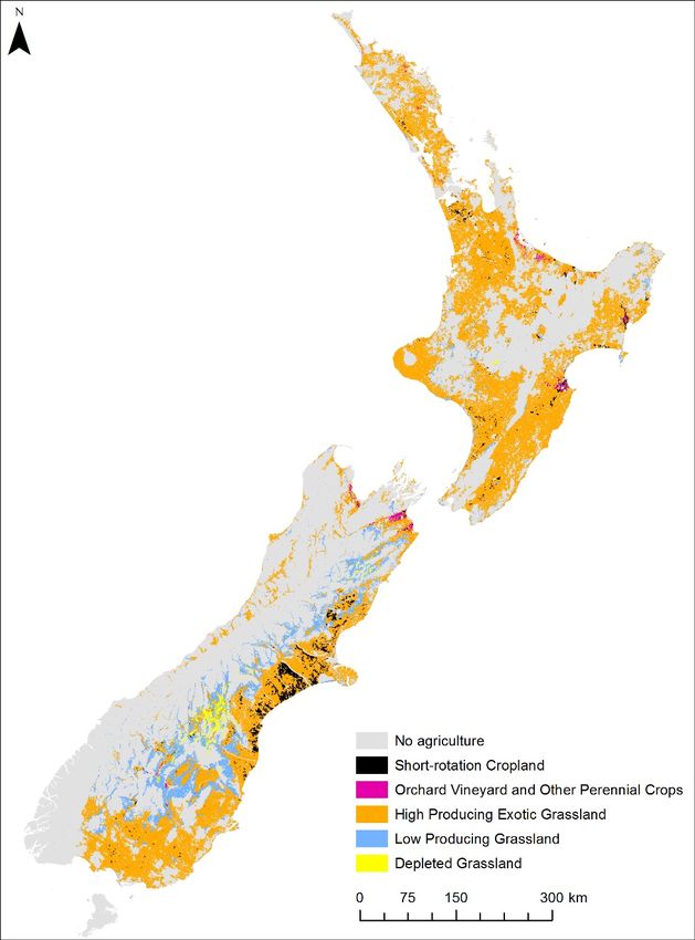
By applying ROA, we will not obtain one strategy but a strategy that can be adjusted over time
depending on the climate change outcomes observed over time, i.e. extending the capacity of the
reservoir. Thus, ROA ensures that resources can be used more efficiently by considering a wide
range of potential outcomes now and determining the best possible strategy for any of these
contingent scenarios.
We use a case study to demonstrate the applicability of ROA as a potential investment appraisal tool
for adaptation to climate. We focus on water availability in the dairy sector, one of the larger
consumers of water resources in New Zealand (Rajanayaka et al., 2010), and which has become
increasingly reliant on water storage over the last two decades. The case study was chosen based
on the following criteria:

  Land cover chosen is dairy dry land to represent the dairy sector;
  The case study should be located in an area that fits the hydrological model
 assumption (i.e. not located in coastal areas where groundwater could play a major
 role);
  The case study should be located in an area that is currently experiencing water stress
 to support agricultural activities;
  The case study should be located in a high productive location where climate changes
 are expected to be relatively consequent and described as follow:
  Mean summer flow is going to decrease by at least 20% (compared to current
 simulated conditions) across all scenarios;
  Summer soil moisture deficit has increased by at least 10% by the end of the Century
 under RCP8.5.

As a result, a catchment was identified in the Canterbury area that meets these criteria in
collaboration with Deep South National Hydrology project team. The catchment is located at nzreach
id 13055784 (branch of Rangitata), approximately 40 km north-west of Hinds in mid-Canterbury
(Figure 4). We stress however, that beyond the selection of the location, all of the other assumptions
are purely hypothetical, i.e. this analysis is not being carried out for an investment decision in reality.

DEEP SOUTH CHALLENGE: CHANGING WITH OUR CLIMATE | 18

Figure 4: Case study location (black outline polygon). Topographic information provided by green
background.

DEEP SOUTH CHALLENGE: CHANGING WITH OUR CLIMATE | 19

5. Data and Methods
In this section we describe the methodology used to carry out the ROA. Before the ROA itself can be
carried out, the hydrological analysis must first be conducted. We describe the data and methods
used for that first, before moving on to describe the ROA method.

 5.1. Climate modelling
Assessing the potential adaptation pathway over the 21st century for primary industry in the face of
impacts of climate change can be carried out using continuous hydrological modelling driven by
climate change projections from a suite of models associated with economic assessment provided by
ROA. The data, models and methods are described below.
The primary input for the hydrological and economic assessments is climate data generated from a
suite of Regional Climate Model (RCM) simulations with sea surface forcing taken from Global
Climate Models (GCMs). These coupled climate models are driven by natural climate forcing such as
solar irradiance and historical and modelled anthropogenic forcing driven by emissions of
greenhouse gases and aerosols based on 4 Representative Concentration Pathways (RCPs), but are
otherwise free-running in that they are not constrained by historical climate observations applying
data assimilation. As part of the fifth IPCC assessment report (AR5) (IPCC 2014), NIWA assessed up to
41 GCMs from the AR5 model archive for their suitability for the New Zealand region. Validation of
those GCMs was carried out through comparison with large scale climatic and circulation
characteristics across 62 metrics (Ministry for the Environment 2018). This analysis provided
performance-based ranking based on New Zealand’s historical climate. The GCMs were then used by
NIWA to drive statistically based regional climate simulations for performing change impact
assessments across New Zealand. The six best performing independent models, where projections
across all four RCPs were available (van Vuuren et al. 2011), were selected for dynamical
downscaling; that is, sea surface temperatures (SST) and sea ice concentrations from the six models
are used to drive an atmosphere-only global circulation model, which in turn drives a higher
resolution Regional Climate Model (RCM) over New Zealand. The output data fields are bias-
corrected relative to a 1980-1999 climatology and subsequently further downscaled to an
approximate 5 km grid (Sood 2014). The RCM output (bias-corrected and downscaled to 5 km) is
then provided as input to a hydrological model which produces soil moisture and river flow.
The NIWA dynamical procedure involves a free-running atmospheric GCM (AGCM) (i.e., not
constrained by historical observations), in this case HadAM3P (Anagnostopoulou et al. 2008), forced
by SST and sea ice fields from the Coupled Model Intercomparison Project Phase 5 (CMIP5) models
(Ackerley et al. 2012). Due to the nature of the climate runs for each GCM, year-to-year variability in
the models does not correspond with observed variability. As such they are a deterministic
consequence of the initial conditions and the solar and anthropogenic drivers. Further details on the
validation of the six GCMs can be found in Sood (2014) and Ministry for the Environment (2018).
Model and parameter uncertainty are discussed in the Uncertainties and limitation section.
The downscaled climate data used here run from 1971 to 2100. From 2005 onward, as per IPCC
recommendations, each GCM is in turn driven by four RCPs that encapsulate alternative scenarios of

DEEP SOUTH CHALLENGE: CHANGING WITH OUR CLIMATE | 20

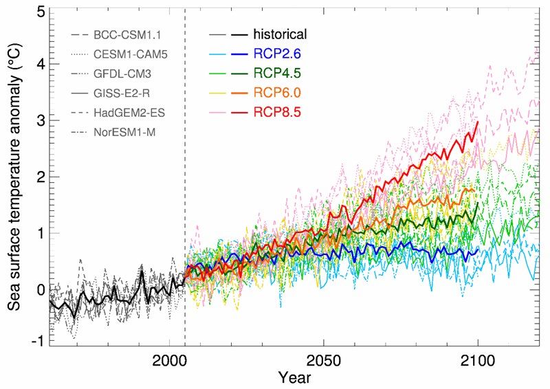
radiative forcing and reflect alternative trajectories of global societal behaviour with regard to
greenhouse gas emissions and other activities. The range of RCPs used can help shed light on the
utility of climate change mitigation. Descriptions and trajectories of the four RCPs are provided in
Table 1 and Figure 5. By mid-century, the temperature trajectory of RCP2.6 is the coolest and RCP8.5
the warmest, with RCP4.5 and RCP6.0 producing intermediate warming. While RCP6.0 ends the
century with more forcing than RCP4.5, early and mid-century it is RCP4.5 that has higher
greenhouse gas emissions and a stronger radiative forcing; this is somewhat reflected by the mid-
century temperature change ranges for the New Zealand seven-station network (Table 1). RCP6.0
overtakes RCP4.5 after the middle of century. The climatic and hydrological effects of the RCPs are
not simply a linear or monotonic progression from the lowest to highest RCP. Furthermore, the
spatial patterns of climatic change across New Zealand are different from RCP to RCP.

Table 1: Descriptions of the Representative Concentration Pathways (RCPs). Temperature changes
are the GCM mean (°C) and, in brackets, the likely ranges.

 Representative Description Seven-station temperature Global surface
 change (Ministry for the temperature change
 Concentration
 Environment 2016) for 2081-2100 (IPCC
 Pathway
 2014, Table 2.1)

 2031-2050 2081-2100

 RCP2.6 The least change 0.7 (0.2, 1.3) 0.7 (0.1, 1.0 (0.3, 1.7)
 in radiative 1.4)
 forcing
 considered, by
 the end of the
 century, with +2.6
 W/m2 by 2100
 relative to pre-
 industrial levels.

 RCP4.5 Low-to-moderate 0.8 (0.4, 1.3) 1.4 (0.7, 1.8 (1.1, 2.6)
 change in 2.2)
 radiative forcing
 by the end of the
 century, with +4.5
 W/m2 by 2100
 relative to pre-
 industrial levels

 RCP6.0 Moderate-to-high 0.8 (0.3, 1.1) 1.8 (1.0, 2.2 (1.4, 3.1)
 change in 2.8)
 radiative forcing
 by the end of the
DEEP SOUTH CHALLENGE: CHANGING WITH OUR CLIMATE | 21

century, with +6.0
 W/m2 by 2100
 relative to pre-
 industrial levels.

 RCP8.5 The largest 1.0 (0.5, 1.7) 3.0 (2.0, 3.7 (2.6, 4.8)
 change in 4.6)
 radiative forcing
 considered, by
 the end of the
 century, with +8.5
 W/m2 by 2100
 relative to pre-
 industrial levels.

Figure 5: Bias-adjusted SSTs, averaged over the RCM domain, for 6 CMIP5 global climate models (2006-
2120), the historical simulations (1960-2005), and four future simulations (RCPs 2.6, 4.5, 6.0 and 8.5),
relative to 1986-2005 (Sood 2015). Individual models are shown by thin dotted or dashed or solid lines (as
described in the inset legend), and the 6-model ensemble-average by thicker solid lines, all of which are
coloured according to the RCP pathway.

DEEP SOUTH CHALLENGE: CHANGING WITH OUR CLIMATE | 22

5.2. Hydrological modelling
In order to assess the potential impacts of climate change on agricultural water resource, a
hydrological model is required that can simulate soil moisture and river flows continuously and
under a range of different climatic conditions, both historical and future. Ideally the model would
also simulate complex groundwater fluxes but there is no national hydrological model capable of this
at present. Because climate change implies that environmental conditions are shifting from what has
been observed historically, it is advantageous to use a physically based hydrological model over one
that is more empirical, with the assumption that a better representation of the biophysical processes
will allow the model to perform better outside the range of conditions under which it is calibrated.
The hydrological model used in this study is TopNet (Clark et al. 2008), which is routinely used for
surface water hydrological modelling applications in New Zealand. It is a spatially semi-distributed,
time-stepping model of water balance. It is driven by time-series of precipitation and temperature,
and of additional weather elements where available. TopNet simulates water storage in the
snowpack, plant canopy, rooting zone, shallow subsurface, lakes and rivers. It produces time-series
of modelled river flow (without consideration of water abstraction, impoundments or discharges)
throughout the modelled river network, as well as evapotranspiration, and does not consider
irrigation. TopNet has two major components, namely a basin module and a flow routing module.
The model combines TOPMODEL hydrological model concepts (Beven et al. 1995) with a kinematic
wave channel routing algorithm (Goring 1994) and a simple temperature based empirical snow
model (Clark et al. 2008). As a result, TopNet can be applied across a range of temporal and spatial
scales over large watersheds using smaller sub-basins as model elements (Ibbitt and Woods 2002;
Bandaragoda et al. 2004). Considerable effort has been made during the development of TopNet to
ensure that the model has a strong physical basis and that the dominant rainfall-runoff dynamics are
adequately represented in the model (McMillan et al. 2010). TopNet model equations and
information requirements are provided by Clark et al. (2008) and McMillan et al. (2013).
For the development of the National TopNet used in this application, spatial information in TopNet is
provided by national datasets as follows:

  Catchment topography based on a nationally available 30 m Digital Elevation Model
 (DEM);
  Physiographical dataset based on the Land Cover Database version two and Land
 Resource Inventory (Newsome et al. 2000);
  Soil dataset based on the Fundamental Soil Layer information (Newsome et al. 2000);
 and
  Hydrological properties (based on the concept of River Environment Classification
 version one- REC1 (Snelder and Biggs 2002).

The method for deriving TopNet’s parameters based on GIS data sources in New Zealand is given in
Table 1 of Clark et al. (2008). Due to the paucity of some spatial information at national/regional
scales, some soil parameters are set uniformly across New Zealand. Because of the model

DEEP SOUTH CHALLENGE: CHANGING WITH OUR CLIMATE | 23

assumptions soil and land use characteristics within each computational sub-catchment are
homogenised. This results in soil characteristics and physical properties of different land uses, such
as pasture and forest, to be spatially averaged, and the hydrological model outputs will be an
approximation of conditions across agricultural land uses.
Hydrological simulations are generated over the period 1971 to 2100, with the spin-up period 1971
excluded from any subsequent the analysis. The climate inputs are stochastically disaggregated from
daily to hourly time steps for model requirements. Hydrological simulations are based on the REC
version 1 network aggregated up to Strahler 1 catchment order three (approximate average
catchment area of 6 km2) to reduce simulation times and data sizes to manageable levels while still
providing useful information; residual coastal catchments of smaller stream orders remain included.
The simulation results comprise hourly time-series of various hydrological variables for each
computational sub-catchment, and for each of the six GCMs and four RCPs considered.
NIWA, in collaboration with Aqualinc, refined the national scale analysis of climate change impacts
on water availability (Collins and Zammit 2016), by considering the effects of climate change alone
on irrigation demand, and by considering when effects may become discernible from or significantly
different to current climate variability (Collins et al 2019). This was carried out by coupling previous
simulations with an irrigation water demand model, IrriCalc (Allen et al. 1998). The assessment
focussed on areas that are currently under irrigation and for simplicity assumed that land use stays
fixed.
As a result of climate change, mean river flows during the irrigation season are projected to increase
across many but not all irrigated areas in the South Island with Southland and parts of Central Otago
showing the first substantial signs by mid-century (2039-2049). Irrigation water demand is projected
to increase across most of New Zealand, with effects emerging by mid-century in the North Island
and later (2080-2099) in the South Island.
From a water management aspect, irrigation restrictions are expected to occur earlier in the year,
mostly for the North Island, but only after the middle of the century and largely only for the extreme
warming scenario. At the same time, irrigation restrictions are expected to stop earlier during the
water year, although the shifts are neither as widespread nor as large as with the change on the
onsets of irrigation restrictions. This shift in the onset and offset of the irrigation restrictions results
in a minimal change in the duration of the irrigations restrictions, but the frequency of irrigation
restrictions tends to increase over the course of the century with the North Island and northern
South Island irrigated areas hardest hit.
Reliability of river water supply (the average fraction of time during each irrigation season that the
river flow is too low and thus irrigation is restricted) tends to decline during the century but largely
only by late-century and for the extreme climate change scenario (Figure 6).

1Strahler order describes river size based on tributary hierarchy. Headwater streams with no tributaries are order 1; 2nd order streams
develop at the confluence of two 1st order tributaries; stream order increases by 1 where two tributaries of the same order converge.
DEEP SOUTH CHALLENGE: CHANGING WITH OUR CLIMATE | 24

DEEP SOUTH CHALLENGE: CHANGING WITH OUR CLIMATE | 25

Figure 6: Mid- and late-century changes in river reliability of supply (Collins et al. 2019).

 5.3. Water demand, water availability and reliability of supply
5.3.1 Water demand and availability
A hypothetical dairy farm of 200 ha in size was used to determine the water demands for this study.
It was assumed that irrigation season spans from September to April. Irrigation water is applied at
90% efficiency to meet the soil-moisture deficit, when water is available. A stock rate of 4 cows/ha
was used with an average daily water demand of 70 litres/day/cow for stock water and dairy shed
cleaning, washing and milk cooling (Stewart and Rout, 2007). We assume that the current stocking
rate and production will continue into the future.
Given that the study area is located within the Canterbury region, Environment Canterbury
allocation rules were used to determine the available water for irrigation and associated activities.
Canterbury Land and Water Regional Plan (ECan, 2017) Rule 5.123.2 states that:
Unless the proposed take is the replacement of a lawfully established take affected by the provisions
of section 124-124C of the RMA, if no limits are set in Sections 6 to 15 for that surface waterbody, the
take, both singularly and in addition to all existing consented takes meets a flow regime with a
minimum flow of 50% of the 7-day mean annual low flow (7DMALF) as calculated by the CRC and an
allocation limit of 20% of the 7DMALF.
Based on the above rule, the minimum flow and primary run-of-river allocation for the stream are
16.6 and 6.7 litres/sec, respectively. It is also assumed that further high stream flows between the
median flow and three times the median flow is available for harvesting and storing in a reservoir.

5.3.2 Reliability of supply and reservoir sizing
Four key factors are generally considered to quantify the reliability of supply-demand (Robb and
McIndoe, 2001). These are:
1. Severity – size or amount of restriction;
2. Frequency – how often the restrictions occur;
3. Duration – how long the restrictions last; and
4. Timing – when restrictions occur.
On any day during the irrigation season, the supply of available water from the storage can be
compared with the demand for irrigation. If water supply from the storage equals or exceeds
demand, reliability is 100%. If demand exceeds water supply, reliability is calculated by dividing
supply by demand to give a supply/demand ratio. The daily ratios can be combined into weekly,
monthly, seasonal (spring, summer, autumn), irrigation season or annual figures.
In general, it is neither economically attractive nor is sufficient water available to develop a large
storage to meet high level of reliability (e.g. >95%) when water is sourced from a small stream.
Therefore, the capacity of the storage has been designed to meet average annual supply/demand
DEEP SOUTH CHALLENGE: CHANGING WITH OUR CLIMATE | 26

ratio of 80%. The unmet demand needs to be met with alternative supplies such as supplementary
feed.

 5.4. The ROA
We begin by providing an overview of the ROA process and the necessary steps, and describe the
relevant methods within each of these.
The ROA decision problem for a multinomial decision-tree method is structured based on the
following steps, following Gersonius et al. (2013) and Dittrich et al. (2019):
1. Specify the decision tree
2. Identify the potential options
3. Formulate the optimisation objective
4. Solve the optimisation problem
5.4.1. Specify the decision-tree

The decision problem can be illustrated in a decision-tree, where the branches represent potential
pathways of available water under the different RCP/GCM combinations. The nodes describe the
water storage sizes constructed, depending on the different water availability outcomes.
For this study we specify a decision tree with two decision-points (2018 and 2050), with four
potential outcomes between 2018 and 2050 and for each of these, a further four potential outcomes
by 2090, when we conclude the analysis. Depending on the type of decision to be made and the
context, more decision points could be selected, but this would increase the complexity. Thus for the
present study we construct a decision-tree with 256 (44) branches.
5.4.2. Determine the probabilities of each branch

Determining the different branches of the decision-tree is one of the major parts of the ROA
methodology, and one of the most challenging and contested in the context of climate change (Kalra
et al. 2014). Most studies make simplifying assumptions that avoid making assumptions regarding
the likelihood of different climate scenarios. Several studies (Abadie et al., 2017; Gersonius et al.,
2013) assume the different climate scenarios are equally likely. Jeuland and Whittington (2014) do
not assign probabilistic weights to the respective scenarios, but transform indicators into relative
measures of downside, expected, and upside performance, but they go on to use Robust Decision
Making (a different approach) to compare across scenarios. Kim et al. (2014) calculate the
probabilities through the standard deviation which are influenced by the percentiles of the rainfall
distribution. However the formula for the volatility assumes that the changes in climate are
normally distributed. Kim et al. (2017) use two RCPs independently, both of which were considered
certain. This does not provide information for considering the likelihood of each RCP. In a very
different approach, Sanderson et al. (2016) use historical climate data from another location as an
analogue for how the climate may become in the case study location.

DEEP SOUTH CHALLENGE: CHANGING WITH OUR CLIMATE | 27

In this study, the combination of RCPs and GCMs provides a 24-members ensemble of potential
futures. To help inform decision-makers concerned with adaptation, it is necessary to define a
conceptual approach that summarises the range of projections in a simpler framework outlining the
range of plausible pathways a key decision variable (in this case water availability) may take. The
term pathway is used to describe the evolution of a single variable over time (i.e. trajectory), not the
propagation of information along a causal chain. This procedure enables probabilities to be assigned
explicitly using “perceived” probabilities to both GCMs and RCPs.
The framework is illustrated hereafter using a probabilistic approach based on the following
assumptions:

  No assessments have been made on the relative plausibility of the six GCMs used thus
 far for climate change projections in the New Zealand region, and so in the absence of
 more specific information we treat each as being equiprobable.
  The relative plausibility or the RCPs, however, are not as unknown. The two end-
 member RCPs (2.6 and 8.5) are both considered less likely than the two middle range
 RCPs (4.5 and 6.0) (see Table 2).

To simplify the application of the framework, while providing enough granulometry for future
decision makers, we collapse the potential 26 futures into 4 states, which correspond to a discrete,
non-overlapping range of simulated hydrological conditions encountered over the time period
considered. For simplicity, the full range of future hydrological conditions is divided in four equal
bins, representing the maximum size of the reservoir needed to meet the water demand over the
time period for the reliability of supply chosen.

Table 2: Two scenarios of relative perceived probabilities for the four RCPs
 RCP Equiprobable Non-
 equiprobable

 2.6 0.25 0.15

 4.5 0.25 0.35

 6.0 0.25 0.35

 8.5 0.25 0.15

5.4.3. Identify the potential options

In this context of this case study, flexibility comes from the size and potential expansion of the
reservoir depending on the future climate. The reservoir sizes in the different time periods are
presented in Table 3.

DEEP SOUTH CHALLENGE: CHANGING WITH OUR CLIMATE | 28

Table 3 - Probabilities and storage sizes for each of the quartile bins, in 2050 and 2090
 2050 2090
 probability probability
 Average Average
 Non- storage Non- storage
 GCM/RCP Equi equi size (m3) GCM/RCP Equi equi size (m3)
 GCM1RCP3 GCM3RCP3
 GCM3RCP4 GCM6RCP1
 GCM2RCP3 GCM3RCP4
 GCM4RCP3 GCM2RCP3
 GCM5RCP4 GCM5RCP1
 0.408
 GCM4RCP1 Bin 1 0.45833 59875 GCM4RCP4
 33 0.541
 GCM3RCP3 GCM3RCP1 Bin 1 0.4817 173500
 7
 GCM3RCP1 GCM1RCP3
 GCM1RCP1 GCM1RCP1
 GCM5RCP1 GCM2RCP1
 GCM1RCP4 GCM3RCP2
 GCM5RCP3 GCM5RCP4
 GCM6RCP2 GCM4RCP3
 GCM4RCP4 0.316 GCM1RCP2
 Bin 2 0.25 117250
 GCM1RCP2 667 GCM6RCP3
 0.208
 GCM3RCP2 GCM6RCP4 Bin 2 0.225 340000
 3
 GCM2RCP2 GCM1RCP4
 GCM6RCP4 GCM5RCP3
 GCM5RCP2 GCM6RCP2
 0.191
 GCM2RCP1 Bin 3 0.20833 174625 GCM2RCP2 Bin 3 0.1417 0.125 506500
 667
 GCM6RCP3 GCM4RCP1
 GCM2RCP4 GCM2RCP4
 GCM6RCP1 0.083 GCM5RCP2 Bin 4 0.1417 0.125 673000
 Bin 4 0.08333 232000
 GCM4RCP2 33 GCM4RCP2

5.4.4. Formulate the optimisation objective

The next step is to formulate the optimisation objective, which is to maximise the net present value
of the storage investment:

 ( )− ( 
 = max ∑ 1=1 (1)
 (1+ ) − 1

DEEP SOUTH CHALLENGE: CHANGING WITH OUR CLIMATE | 29