WP/20/116 It is Only Natural: Europe's Low Interest Rates (Trajectory and Drivers) - International Monetary Fund

WP/20/116

 It is Only Natural: Europe’s Low Interest Rates
 (Trajectory and Drivers)

 by Marco Arena, Gabriel Di Bella, Alfredo Cuevas,
 Borja Gracia, Vina Nguyen, and Alex Pienkowski

IMF Working Papers describe research in progress by the author(s) and are published
to elicit comments and to encourage debate. The views expressed in IMF Working Papers
are those of the author(s) and do not necessarily represent the views of the IMF, its
Executive Board, or IMF management.

© 2020 International Monetary Fund 2 WP/20/116

 IMF Working Paper

 European Department

 It Is Only Natural: Europe’s Low Interest Rates (Trajectory and Drivers)

 Prepared by Marco Arena, Gabriel Di Bella, Alfredo Cuevas, Borja Gracia, Vina
 Nguyen, and Alex Pienkowski

 Authorized for distribution by Jörg Decressin

 June 2020

Disclaimer: This document was prepared before COVID-19 became a global pandemic and resulted in
unprecedented economic strains. It, therefore, does not reflect the implications of these developments and
related policy priorities. We direct you to the IMF Covid-19 page that includes staff recommendations
with regard to the COVID-19 global outbreak.

 IMF Working Papers describe research in progress by the author(s) and are published to
 elicit comments and to encourage debate. The views expressed in IMF Working Papers are
 those of the author(s) and do not necessarily represent the views of the IMF, its Executive Board,
 or IMF management.

 Abstract

Estimates of the natural interest rate are often useful in the analysis of monetary and other
macroeconomic policies. The topic gathered much attention following the great financial
crisis and the Euro Area debt crisis due to the uncertainty regarding the timing of monetary
policy normalization and the future path of interest rates. Using a sample of European
countries (including several members of the Euro Area), this paper provides estimates of
country-specific natural interest rates and some of their drivers between 2000 and 2019. In
line with the literature, our findings suggest that natural interest rates declined during this
period, and despite a rebound in the last few years of it, they have not recovered to their pre-
crisis levels. The paper also discusses the implications of the decline in natural interest rates
for monetary conditions and debt sustainability.

JEL Classification Numbers: E4, E5, H6, C1

Keywords: Natural interest rate, Neutral interest rate, monetary policy, debt sustainability,
Bayesian estimation

Authors’ E-Mail Addresses: MArena@imf.org; GDiBella@imf.org; ACuevas@imf.org;
BGracia@imf.org; HNguyen3@imf.org; APienkowski@imf.org;

3

 Content

Abstract....................................................................................................................................2

I. Introduction..........................................................................................................................4

II. The Natural Rate................................................................................................................5

III. Estimation Methodologies and Results...........................................................................7

IV. Policy Implications..........................................................................................................20

V. Conclusion........................................................................................................................27

Figures:
1. Natural Interest Rates with Z Modelled as a Random Walk...............................................10
2. Natural Interest Rates with Z Modelled as a Function of Other Variables..........................13
3. Natural Interest Rate Trend (z) Decomposition...................................................................14
4. Natural Interest Rates Using Factor Models........................................................................17
5. Co-movements in r* and g in the Euro Area.......................................................................18
6. Market Expectations of the Real Rate.................................................................................19
7. Monetary Conditions...........................................................................................................23
8. Monetary Conditions and Fiscal Policy...............................................................................25

Annexes:

I. Defining the Natural Rate.....................................................................................................33
II. Technical Details on the L-W Model..................................................................................36
III. Model Priors: Review of the Literature.............................................................................39
IV. Prior and Posterior Distributions of Parameter and Shock Estimates...............................42
V. Technical Details on Factor Models...................................................................................47
VI. Background Figures and Tables........................................................................................52

References................................................................................................................................29

4

 I. INTRODUCTION 1

The last decade saw a revival in the interest, at both the academic and policy level, in the real
natural interest rate, r*. This revival can be explained by the desire to assess the effectiveness
of monetary policy in an environment of very low interest rates since the global financial
crisis (GFC). And to form a view about the future path of interest rates, including because of
their role in shaping public debt dynamics.

The very upheaval in the global economy that stimulated interest in this topic, however,
complicates the empirical estimation of r* and its drivers. The GFC left a legacy of
historically low observed real interest rates; but separating cycle from trend in this
environment is especially difficult. This adds to the intrinsic statistical uncertainty related to
estimating, and even defining, a non-observable variable. This suggests the need to use a
variety of analytical approaches (even if this implies subtly different underlying concepts of
r*) and handling any results with caution. The focus of this paper is on applying a few
different approaches to the estimation of r* over the last two decades in a diverse group of
European countries (France, Germany, Italy, Lithuania, the Netherlands, Poland, Portugal,
Romania, Russia, and Spain). The estimates of r* use easily replicable models, which are
flexible enough to be applied to economies with different structures and fundamentals.

The heterogeneity of our sample provides an opportunity to explore some questions related to
the determinants of r*, such as the role of membership in a currency union, the influence of
(often volatile) capital flows, or the different impact of a similar shock on advanced vis-à-vis
emerging economies. Our results also help us characterize the stance of monetary policy
during periods of interest, such as the run-up to, and the aftermath of the GFC. While the
period covered in this study is prior to the COVID-19 crisis, our conclusions on r* (their
country specific level and their determinants) allow us to discuss some factors that may have
a bearing on the future level of interest rates, as well as their broad policy implications,
including for fiscal sustainability.

All methodologies applied in this paper find a generalized decline in r* over the last 20 years,
particularly in advanced economies. That said, estimates based on economic models that
explicitly link r* to developments in the real economy show some partial recovery in recent
years, as growth resumed following the crisis. In contrast, statistical models that focus more
narrowly on the time series behavior of interest rates show a continuing decline in the natural
rate since the end of the crisis. This divergence underscores the uncertainty about the current
value of the natural rate and its future path—although none of our estimates points to clear
prospects for natural rates increasing.

1
 Excellent research assistance by Yuanchen Cai and Boyang Sun is gratefully acknowledged. We also thank
Andrea Pescatori, Carolina Osorio Buitron, Vassili Bazinas, and Etienne Vaccaro-Grange for their help with
various model codes. We benefited greatly from discussions with, or specific comments from Marco Casiraghi,
Mai Dao, Jorg Decressin, Enrica Detragiache, Lucyna Gornicka, Rishi Goyal, Lucy Liu, Meera Louis, Jean
Marc Natal, Natalia Novikova, Ara Stepanyan, Marzie Taheri, Sebastian Weber, Jing Zhou, and participants in
seminars in IMF European Department and the 2019 IMF Annual Meetings.

5

Empirical estimates of the difference between the (real) policy rate and r* (an unobservable
variable) can be used to assess the stance of monetary policy in different places and at
different times. We find that differences in r* across countries lead to significant
heterogeneity in monetary conditions within the Euro Area during the last two decades, even
though these countries operate under a single monetary policy aimed at the Euro Area as a
whole. 2 By the end of our sample, though, monetary conditions were highly accommodative
in all Euro Area countries. In emerging Europe, there has been a propensity to pursue pro-
cyclical polices (particularly in Russia), largely due to the complicated role of the risk
premium. More generally, a persistently low r* across Europe, and notably in the Euro Area,
suggested that unconventional monetary policies (UMPs) may become much more
conventional in the future. In terms of fiscal policy, a lower r* does provide some fiscal
space on public sector balance sheets—some of which was already being used by several
countries by the end of our sample period. But declining potential growth towards the end of
this period and already high debt in many countries suggested that country authorities needed
to be cautious about accumulating more debt.

The remainder of this paper is organized as follows. Section II discusses common definitions
of the natural interest rate, issues related with its measurement, and elements to consider in
advanced and emerging economies. Section III presents the methodologies we use to
estimate natural rates, and our results. Section IV discusses policy implications, and Section
V concludes.

 II. THE NATURAL RATE

The natural (or neutral, as it is also often called) rate of interest, r*, like potential output or
the non-accelerating inflation rate of unemployment (NAIRU), is an unobservable variable.
There are many definitions of r* beginning with Wicksell’s in the late XIX century. These
definitions typically refer to some idea of equilibrium. But they may differ in important
details such as the specific equilibrium conditions one has in mind (including, importantly,
for the behavior of prices or inflation), the stability of such an equilibrium, the emphasis
placed on dynamics outside equilibrium, the weight placed on supply- or demand-side
factors, and the time horizon under consideration. These differences make it easy for two
economists to use the same term, “natural rate,” while referring to subtly different ideas (see
Annex I).

In this paper, r* is defined as the rate that maintains an economy in equilibrium if it starts
there and does not interfere with the autonomous return to equilibrium of an economy
initially in disequilibrium. This notion includes the common definition of r* as the real
interest rate that would prevail if the output gap were closed and inflation stable. Our view of

2
 Among the Euro Area countries in our sample, Lithuania was not a founding member of the EMU, which it
joined on January 1, 2015. However, since February 2002, Lithuania pegged its currency to the euro in the
context of the ERM II, operating a currency board framework and allowing the use of the euro in settlement of
transactions in its territory. For this reason, it is treated as a Euro Area country in this paper.

6

the natural rate admits variation in the near term in response to changing conditions in the
real economy, but also can be expected to settle around some central value (or trajectory) in
the longer term—a value that will be related to the steady state rate of growth of the
economy. This will become clearer in the following section, as we present the models used in
estimation.

Estimating r* Empirically

We assume that r* is a short-run interest rate, such as the overnight rate or the 3-month
government bill rate. This is consistent with a large part of the literature, which typically
looks for the “natural” level r* of some real short-term rate r, such as the (properly deflated)
rate on short term government debt instruments or the inter-bank overnight interest rate. In
some papers, especially those focusing on reserve currency issuers (the U.S., U.K., Japan and
the Euro Area), r* is associated to the idea of a risk-free rate, often that of government bill or
the central bank policy rate. Importantly, in such contexts, r* cannot be viewed as the
average return on capital in an economy, which typically includes credit and duration risk. As
noted by Brand et al (2018), while the real return on capital has been stable or rising in the
Euro Area, most measures of r* have been declining. They attribute this divergence to rising
risk aversion or higher profit margins, among other factors.

Capital Account and Other Considerations

In an economy with an open capital account, r* should also ensure the no-arbitrage condition
between real returns on domestic and foreign assets (real uncovered interest parity). Thus,
this concept also includes equilibrium in the capital account. In fact, the view of r* as risk-
free is less plausible when considering non-reserve currency issuers with an open capital
account. In such cases, domestic currency-denominated securities are typically subject to
significant exchange rate risk, as resident and non-resident economic agents change their
portfolio composition as a response to news signaling, for instance, a more likely
appreciation (or depreciation) of the real exchange rate. Indeed, an open capital account in a
small economy gives rise to new problems in defining an equilibrium interest rate. 3 In such a
context, lower policy rates may not be available to stimulate a weak economy if economic
agents are re-pricing domestic risk. In fact, this is a trade-off faced frequently by
policymakers in emerging markets (Rey, 2015). If policy rates are permanently high because
of these considerations, then the corresponding r* should be also permanently elevated. This
means that real exchange rate uncertainty and country risk premia can push the natural rate
upwards in emerging economies, as capital mobility ensures that risk-adjusted real returns
are arbitraged. This trade-off is explored empirically in Section III, where we discuss
emerging market countries with currencies of their own.

3
 Different real exchange rate levels may also bring about the possibility of default and currency
inconvertibility, among other factors, which further complicates the definition of equilibrium interest rates in
emerging economies.

7

Natural Rates in a Currency Union

Considering r* in a currency union also raises interesting conceptual issues. A general
assumption in theoretical models is that in the long-term monetary variables should not affect
real variables such as potential growth or r*. Thus, in principle, r* could differ among the
members of a currency union if they are subject to asymmetric (domestic and external)
shocks, even though they are subjected to a single monetary policy aimed at attaining a given
inflation target in the union as a whole. Similarly, a monetary union should not necessarily
accelerate convergence, except to the extent that it pushes factors of production to become
more homogenous, substitutable and mobile. Again, there need not be a common equilibrium
r* within a currency union. In the face of heterogeneous r* rates, a common monetary policy
will result in different monetary conditions in each member state, possibly during long
periods of time. That said, it is possible to expect some r* co-movements in countries that
belong to monetary union; such co-movements could change over time, an issue that we
explore later in the paper.

 III. ESTIMATION METHODOLOGIES AND RESULTS

A consensus exists that there was a global decline in r* over the last two decades (Summers,
2014; Holston et al, 2017; Brand et al, 2018 and Del Negro et al, 2019). Rachel and Smith
(2015) document a decline in the global long-term r* of around 450 bps since 1980. 4 They
argue that this decline is difficult to explain only by changes in global growth (to which
changes in r* are usually thought to be related), and that shifts in saving and investment
preferences have played an important role. In their view, negative demographic forces,
higher inequality within countries, and increased desired savings by emerging market
governments have increased desired saving. And a decline in the relative price of capital,
lower public investment projects, and the increasing spread between the rate of return on
capital and the risk-free rate, have reduced desired investment. In this section we apply a
variety of methodologies to produce specific estimates for a sample of European countries,
both inside and outside the Euro Area, that speak to these issues.

The Laubach-Williams Model and its Variants

The seminal Laubach and Williams (2003) model (L-W model) is the benchmark framework
to estimate r*. In this model, r* is allowed to vary from one period to the next in response to
shocks that take place at short term frequencies. The resulting estimates reflect a tension
between demand and supply side considerations, represented by equations that capture
demand behavior and the fundamental linkage between r* and potential growth, as well as a
Phillips curve, allowing the simultaneous estimation of r* and potential growth (g) from
observable data using a Kalman filter. This framework is often viewed as producing a

4
 Magud and Tsounta (2012) find that the natural rate of interest has declined in many Latin American countries
over the last decade.

8

medium-term equilibrium estimates, because r* is modeled as influenced by factors that
change relatively slowly. The original L-W model was calibrated to fit the US economic
data; a more recent version can be found in Holston et al. (2016), which covers more
countries. What follows is a summary of the model (more details in Annex II).
The model has a backward-looking IS-Curve that relates the current value of the output gap
( � ) to its own lags, and to the difference between the prevailing real interest rates and the
natural level ( − ∗ ):
 
 � = 1 � −1 − 2 ( − ∗ )+ (1)

In expression (1), the prevailing real rate ( ) is assumed to be exogenous to the framework in
the short run. In other words, is assumed as policy determined, without explicitly modeling
a policy reaction function, and to be equal to the difference between the nominal policy rate
 
( ) and one-year ahead (country specific) inflation expectations ( +1 ), while is a random
shock. Expression (1) suggests that the estimated evolution of the output gap over time,
together with the observed path of the real interest rates, can be used to infer something about
the trajectory of the natural rate ∗ . 5

As usual, the output gap is equal to the difference between (log) realized real output ( ) and
its potential ( ), with the change in the latter assumed to be driven by trend growth ( ) and
a random i.i.d. shock ( ):

 = −1
 
 + + , (2)

In turn, is modeled as a random walk with innovations :
 
 = −1 + . (3)

The model also includes an open-economy backward looking Phillips Curve relating
inflation ( ) to its own lag, to � and to import price inflation :
 
 = 1 −1 + 2 � −1 + 3 −1 + , (4)

where is assumed to be exogenous and is an i.i.d. shock.

5
 As ∗ is proxied by a short-term interest rate, the estimation using expression (1) (IS curve) assumes that
equilibrium in the goods market can be achieved by changing, say, the three-month interest rate. However, this
may not be the case, as in protracted financial crisis where lower interest rates may be needed along the yield
curve.

9

The model imposes a linear relationship between natural rates and potential output growth,
capturing the theoretical idea that they share some of their main drivers; that is, r* is allowed
to reflect supply side developments. But the specification permits the paths of trend growth
and r* to diverge. In this simple setting, the determinants of ∗ are trend growth, , and an
exogenous process, , capturing other possible determinants of r* which may create a wedge
over time between r* and g. Trend growth and r* are linked by a constant, > 0.

 ∗ = + (5)

In the simplest version of this model, follows a random walk with iid shocks ( ). 6 As it
follows from expressions 1–5, this framework does not directly allow monetary policy to
explain the behavior of the natural interest rate.

We follow Pescatori and Turunen (2015) and estimate the model parameters using Bayesian
techniques. This choice allows to circumvent the “pile-up” problem in classical inference and
gives the analyst some additional control over the estimation procedure. 7 In particular, the
 
prior assumptions on the variance of the error terms on , and are important, as they
influence how the variance of r* responds to (the level and trend) shocks to potential growth
and to the unexplained component, . In other words, they influence how closely the
estimated r* follows estimates of g. 8 In addition, we will try different variations of the
specification for the term in expression (5), starting with a random walk and moving to
more complex but potentially more economically interesting specifications. Others in the
literature have followed similar approaches (Laubach and Williams (2003) and (2016); Lewis
and Vazquez-Grande (2017), Holston et al (2017), among others), facilitating the comparison
between their results and ours. 9

Figure 1 shows our first set of estimates (specifying as a random walk) for both Euro Area
countries and emerging Europe. Our results suggest that r* declined over the last two decades

6
 As part of the estimation process, the output gap found in expressions (1) and (4) would typically be estimated
with the rest of the unobserved variables in the model. An alternative is to consider as “data” a measure of the
output gap estimated outside the L-W framework, treating it as a noisy signal of the endogenously determined
output gap. When estimating r* below, we will use output gaps estimated by IMF desk economists and reported
in the World Economic Outlook (WEO) as an additional signal to estimate our own output gap in the Laubach
and Williams framework. See Annex II.
7
 The “pile-up” problem affects inference around unit roots. In the L-W framework, the “pile-up” problem
arises in the estimation of trend growth and exogenous factor variances, because the variation of the trend
component is much smaller than that of the cyclical component, making the trend variance estimate to be biased
towards zero. With Bayesian methods, the pile-up problem of inference around unit roots is not as severe.
However, the role of the priors and the assumed covariance structure of the exogenous shocks is magnified in
the presence of unit roots (see Stock (1991)).
8
 Annex III describe the implications of these priors for the level and volatility of r* estimates.
9
 Beyer and Wieland (2017) or Mésonnier and Renne (2007) highlight that the random walk assumption for 
leads to very unstable results. Like Pescatori and Turunen (2015) and Hakkio and Smith (2017), we include
some economic drivers of in a stationary process.

10

in virtually all countries in our sample, both in the Euro Area and outside, with some modest
recovery post-Euro Area Debt Crisis (2012). As the Figure 1 (and those in Annex VI)
suggests, both natural rates and potential growth rates have fallen relative to the early 2000s
in most places, despite some recovery in the last several years (Germany seems an exception,
with a remarkably stable estimated potential growth). But r* typically fell more markedly
than potential growth in the course of the last two decades, particularly after the GFC. For
Euro Area countries, the average decline in r* was 2 percentage points since 2000, with r*
estimated at a value of around zero in 2019:Q1. For emerging Europe there is also a decline
in r*, which is larger in Russia (around 4 percentage points) compared to that in Romania
and Poland (around 1 percentage point) since the early 2000s. The part of the decline in r*
that seems to be explained by the fall in g is generally smaller in Euro Area countries than in
emerging economies; in this regard, Russia stands out for having the largest decline in r*
combined with the closest linkage to a change in g.

 Figure 1. Natural Interest Rates with Z Modelled as a Random Walk
 Euro Area: Natural Interest Rates Italy - Components of Natural Rate of Interest
 (Percent; Z process modelled as a random walk)
 2
 8 g*
 FRA ITA
 6 DEU ESP Unexplained residual
 1
 PRT LTU r*
 4
 NLD
 2 0
 0
 -2 -1
 -4
 -6 -2
 2000Q1
 2001Q1
 2002Q1
 2003Q1
 2004Q1
 2005Q1
 2006Q1
 2007Q1
 2008Q1
 2009Q1
 2010Q1
 2011Q1
 2012Q1
 2013Q1
 2014Q1
 2015Q1
 2016Q1
 2017Q1
 2018Q1
 2019Q1
 2000Q1
 2001Q2
 2002Q3
 2003Q4
 2005Q1
 2006Q2
 2007Q3
 2008Q4
 2010Q1
 2011Q2
 2012Q3
 2013Q4
 2015Q1
 2016Q2
 2017Q3
 2018Q4

 Emerging Europe: Natural Interest Rates Poland - Components of Natural Interest Rate
 (Percent; Z process modelled as a random walk)
7 6
 g*
6 5
 Unexplained residual
 4
5 r*
 3
4
 2
3
 1
2
 0
1 ROU POL RUS -1
0 -2
 2000Q1
 2001Q2
 2002Q3
 2003Q4
 2005Q1
 2006Q2
 2007Q3
 2008Q4
 2010Q1
 2011Q2
 2012Q3
 2013Q4
 2015Q1
 2016Q2
 2017Q3
 2018Q4

 2001Q1
 2002Q1
 2003Q1
 2004Q1
 2005Q1
 2006Q1
 2007Q1
 2008Q1
 2009Q1
 2010Q1
 2011Q1
 2012Q1
 2013Q1
 2014Q1
 2015Q1
 2016Q1
 2017Q1
 2018Q1
 2019Q1

 Sources: Authors' calculations.

11

These estimates suggest that the decline in natural rates cannot be attributed to the slowdown
in trend growth alone, especially post-GFC. 10 Annex VI shows the decomposition of r*
between trend growth and for all countries in our sample, and Figure 1 above includes one
advanced economy and one emerging market for illustration purposes. The decline in r* in
most Euro Area countries in our sample before the GFC seems to have been driven by
weakening trend growth to a large extent, but not fully. After the GFC, however, trend
growth picks up somewhat, but r* continues to fall, at least for a while, opening a wide
wedge between r* and g. 11 This points to an increasing role of other factors in determining r*
(summarized by ). Indeed, for most Euro Area countries in our sample, around half of the
overall estimated decline in r* since the GFC can be attributed to the behavior of the
unexplained component, . In Portugal and Spain, the importance of this z component is the
largest, with the wedge between r* and g rising to 3–4 percentage points around the time of
the Euro Area Debt Crisis. 12 In recent years, r* has picked up somewhat, seemingly spurred
by the recovery in potential growth.

For emerging Europe, the association between r* and g seems stronger than in the Euro Area,
although there is a moderately increasing wedge between r* and g after the GFC in Poland
and Romania. In the case of Russia, we estimate a value for r* of around 2 percent in early
2019, broadly similar to our estimate for trend growth. These estimates are not far from those
in Kreptsev et al. (2016) and are also broadly similar to those estimated by the Central Bank
of Russia’s (CBR) (2–3 percent). In the case of Poland, contributes negatively to r* with
its value increasing from about zero in the early 2000s to about 1 percentage point (in
absolute terms) by early 2019, with most of that increase occurring during and after the GFC.

But what could account for the wedge between r* and g? What economic factors might be
behind the estimated trajectories of ? To explore this unexplained component, we model 
as a function of some economic variables and autoregressive terms which seem justified by
the rather persistent behavior of in our initial estimates. As the economies in our sample
are open, the explanatory variables that we add aim to reflect external factors. Concretely, for
the Euro Area we assume a process for of the following form:

10
 Our results refer to the median estimates for r* at each point. The distribution around the median for all
countries are available upon request.
11
 The estimate of the coefficient c in the expression for r* is around unity, which makes it possible to loosely
refer to as wedge the between r* and g.
12
 Spain’s r* in Figure 1 shows a somewhat atypical behavior, especially in the two years before the GFC, when
it rises. This might reflect the positive and increasing output gap estimated in the WEO, which would have
called for tighter monetary conditions at the time. The dip following the euro area is pronounced, but not
atypical. In contrast with our results, Brand et al. (2018) showed that Spain’s r* declined from about 2.0–2.5
percent before the crisis to about -0.2 percent during the European debt crisis. Fries et a. (2017) found that the
r* for Spain dropped to about -1.5 percent during the crises.

12

 = 1 −1 + 2 −2 + Δ + + Δ + (6)

where Δ is the difference between the actual level of the REER and its trend, is
trading partner growth representing external demand, and is the difference between
the 10-year country’s government yield relative to Germany’s 10-year government yield (for
Germany we use Credit Default Swaps, CDS). 13 While the first two are designed to reflect
the influence of the current account, the spreads can be seen both as a measure of risk and as
a proxy for the influence of the capital account on domestic conditions.

For emerging Europe, we use the following specification:

 = 1 −1 + 2 −2 + Δ + ΔEMBI + Δ + (7)

where Δ refers to 10-year Treasury Bond yield at constant maturity deflated by the
expected inflation rate, Δ is the Emerging Market Bond Index spread (EMBI, which is
usually understood to represent country risk), and Δ refers to the news-based index
of economic policy uncertainty developed in Baker, Bloom, and Davis (2016). In emerging
Europe, short-term REER fluctuations should be associated with both changes in economic
policy uncertainty, which affect international financial flows, and with changes in the terms
of trade, which affect the current account. 14

The inclusion of these additional factors increases the volatility of our r* estimates for Euro
Area countries (Figure 2 and Annex VI.2). In particular, the drops in r* in 2009 and 2012 are
steeper, and the subsequent recoveries are also more pronounced. However, the estimated
overall decrease in r* over the last two decades is broadly similar regardless of how we
model (See Annex VI), and large residuals remain in some cases. The fact that the latest
estimates of r* are broadly similar no matter whether is modelled as in equation (6) or not
may suggest that domestic conditions (possibly related to factors that had a lasting impact in
the second decade of this century, such as dealing with debt overhangs in the private and
public sectors) play a strong role.

Broadly speaking, these results are also consistent with other estimates in the literature.
Brand el al (2018) bring together several estimates of r* for the entire Euro Area. These
estimates are concentrated between 0 and -1percent, which encompasses our estimate of
individual Euro Area countries (except Lithuania). Fries et al (2017) jointly estimate r* for

13
 Pescatori and Turunen (2015) use similar specifications to model .
14
 Since the country-specific policy uncertainty index is not available for Poland and Romania, we use the
European policy-related economic uncertainty for these countries. In addition, we have also run an alternative
specification that replaces such index with the REER. To gain intuition how the REER or policy uncertainty
may change the level of the natural rate, consider an economy that is subject to persistent shocks to its terms of
trade, resulting in domestic consumption volatility and potentially affecting sovereign payments (i.e., affecting
policy uncertainty). In such a case, the covariance between consumption and the REER would be negative,
prompting a positive wedge between expected real returns of domestic-denominated instruments and those of
foreign interest rates, which covariate much less with domestic consumption.

13

Spain, Italy, France, and Germany. Their estimates show much closer co-movement between
the economies, but they also find a similar magnitude in the decline of r* over the last two
decades, and find r* to be close to zero as of end-2017.

 Figure 2. Natural Interest Rates with Z Modelled as a Function of Other Variables 1/

 Euro Area: Natural Interest Rates Italy: Decomposition of Z
 (Percent; Z process modelled as a function of Spread, (Percent; Z process modelled as a function of Spread,
 External demand, and REER) External demand, and REER)
 6 1
 4
 2 0
 0
 -2 -1 Spread

 -4 External demand

 -2 REER
 -6 FRA ITA DEU ESP
 PRT LTU NLD Residual
 -8
 z
 -3
 2000Q1
 2001Q2
 2002Q3
 2003Q4
 2005Q1
 2006Q2
 2007Q3
 2008Q4
 2010Q1
 2011Q2
 2012Q3
 2013Q4
 2015Q1
 2016Q2
 2017Q3
 2018Q4

 2000Q1
 2001Q2
 2002Q3
 2003Q4
 2005Q1
 2006Q2
 2007Q3
 2008Q4
 2010Q1
 2011Q2
 2012Q3
 2013Q4
 2015Q1
 2016Q2
 2017Q3
 2018Q4
 Emerging Europe: Natural Interest Rates Russia: Decomposition of Z
 (Percent; Z process modelled as a function of EMBI, US (Percent; Z process modelled as a function of EMBI, US
 rate, and Policy uncertainty) rate, and Policy uncertainty)
4.5
 1.5
4.0
3.5 1.0
3.0 0.5
2.5
2.0 0.0

1.5 -0.5
1.0 EMBI US rate
 -1.0 Policy uncertainty Residual
0.5 ROU POL RUS
 z
0.0 -1.5
 2000Q1
 2001Q2
 2002Q3
 2003Q4
 2005Q1
 2006Q2
 2007Q3
 2008Q4
 2010Q1
 2011Q2
 2012Q3
 2013Q4
 2015Q1
 2016Q2
 2017Q3
 2018Q4

 2002Q1
 2003Q1
 2004Q1
 2005Q1
 2006Q1
 2007Q1
 2008Q1
 2009Q1
 2010Q1
 2011Q1
 2012Q1
 2013Q1
 2014Q1
 2015Q1
 2016Q1
 2017Q1
 2018Q1
 2019Q1

 Sources: Authors' calculations.
 1/ The contribution of the explanatory variables shows the cumulative contribution over three
 quarters as each variable and the z process are assumed to follow an AR(2) process. The
 residual includes the shock to z this period and the lagged residual from the past two quarters.

Looking more closely, our results also suggest that variations in spreads have been at times
responsible for large movements in r* in some Euro Area countries. Take Lithuania and Italy
for example (Figure 3). In 2009 at the lowest point in Lithuania’s recession, the credit crunch
(as proxied by the sharp rise in spreads), contributed to a fall in r* of 2 percentage points.

14

That is, a much lower real interest rate would have been needed to achieve a closed output
gap and stable inflation in those stressed circumstances. The improvement in fundamentals
that followed this period allowed Lithuania to avoid significant spillovers from the Euro Area
debt crisis and resulted in a dramatic improvement in credit conditions. In turn, Italy saw a
deep fall in r* associated with worsening spreads, driven by heightened uncertainty around
debt sustainability at the height of the Euro Area Debt Crisis, as well as a smaller
deterioration in recent quarters. Annex VI shows similar developments in Portugal and Spain.
Moreover, Figure 3 (and Annex VI) show that while REER changes do not explain much of
 in most Euro Area countries, external demand changes appear to result in sharp declines in
r* during the GFC, especially for export-oriented economies like Germany or the
Netherlands. In these countries, the collapse in external demand in 2009 resulted in a
3 percentage point decline in r*, later reversed as external demand rebounded, illustrating the
volatility of r* and its sensitivity to external shocks.

 Figure 3. Natural Interest Rate Trend (z) Decomposition
 Contribution of External Demand to r* Contribution of spreads to r* 1/
 1.0 1.0
 0.5
 0.5
 0.0
-0.5 0.0
-1.0
 -0.5
-1.5
-2.0 FRA ITA -1.0 FRA ITA
-2.5 DEU ESP DEU ESP
 PRT LTU -1.5 PRT LTU
-3.0
 NLD NLD
-3.5 -2.0
 2000Q1
 2001Q2
 2002Q3
 2003Q4
 2005Q1
 2006Q2
 2007Q3
 2008Q4
 2010Q1
 2011Q2
 2012Q3
 2013Q4
 2015Q1
 2016Q2
 2017Q3
 2018Q4
 2000Q1
 2001Q2
 2002Q3
 2003Q4
 2005Q1
 2006Q2
 2007Q3
 2008Q4
 2010Q1
 2011Q2
 2012Q3
 2013Q4
 2015Q1
 2016Q2
 2017Q3
 2018Q4

 1/ Spreads refer to ten-year bond yield spread between each
 country and Germany, except in the case for Germany itself,
 spread refers to the CDS spread

 Contribution of US Rate to r* 1/ Contribution of Country Risk to r* 1/
 0.6 1
 0.4 0.8
 0.2
 0.6
 0
 0.4
-0.2
 0.2
-0.4
-0.6 0
-0.8 -0.2
 -1 -0.4
 ROU POL RUS
-1.2 -0.6 ROU POL RUS
 2001Q1
 2002Q2
 2003Q3
 2004Q4
 2006Q1
 2007Q2
 2008Q3
 2009Q4
 2011Q1
 2012Q2
 2013Q3
 2014Q4
 2016Q1
 2017Q2
 2018Q3
 2001Q1
 2002Q1
 2003Q1
 2004Q1
 2005Q1
 2006Q1
 2007Q1
 2008Q1
 2009Q1
 2010Q1
 2011Q1
 2012Q1
 2013Q1
 2014Q1
 2015Q1
 2016Q1
 2017Q1
 2018Q1
 2019Q1

 1/ Rate here refers to the US 10-year real soverign yield, 1/ The difference between the Emerging Market Bond
 measured as the difference between the nominal yield Index and the US 10-year real sovereign yield.

 Sources: Authors' calculations.

15

As noted, even after we model as a function of economic variables, there remains a
relatively large unexplained component of r* for most Euro Area countries (Figure 2 and
Annex VI). This may reflect a common factor influencing r* (Jordà and Taylor, 2019),
coupled with country-specific factors. These could include fiscal shocks (Rachel and
Summers, 2019), the slow deleveraging process following the GFC, and financial cycles
(Belke and Klose, 2018; Borio et al, 2019). In addition, a growing body of literature
discusses the importance of demographics. Brand et al. (2018) and Bielecki et al. (2018)
emphasize the role of demographic trends, which could extend beyond their impact on
growth itself. Depending on which of these factors are thought to be most relevant, one’s
view of the future path of interest rates may be affected. For example, if one thinks that the
unexplained part of (and r*) reflects the protracted deleveraging process, there may be
room for the wedge between r* and g to diminish further over time (testing this conjecture,
however, remains part of the agenda for future work).

As in the Euro Area countries, r* estimates for emerging Europe are more volatile when
modeling as a function of economic variables. The volatility of r* increases following
global shocks affecting Emerging Economies (like the “taper tantrum”), or country-specific
shocks (like the dual shock of western sanctions and lower oil prices for Russia in 2014–
15). 15 A decomposition of the exogenous variables affecting r* shows that effects from the
decline in the U.S. long-term interest rate have pushed r* downwards, while increases in
country risk premium (as measured by the EMBI) pushed r* upwards. This impact on r* of
changes in the EMBI is in contrast with the impact of changes in the 10-year spread in Euro
Area countries such as Portugal or Spain. This reflects in part deliberate choices in the
empirical implementation of the model and should thus be taken with some caution (see the
prior distributions of the relevant parameters in annex IV). A motivation for these choices is
the role of interest rates in affecting external equilibrium in an emerging economy with a
currency of its own. In addition, the use of specification (9) in the case of Russia shows that
the negative impact on r* of decreases in global interest rates and reductions in country risk
has been more than offset by increases in the perception of economic policy uncertainty,
which explains a large part of (see Figure 2 and Annex VI). In turn, considering the REER
instead of policy uncertainty suggests that the contribution of the former to r* is small, which
may be reflecting a correlation of the exchange rate with the other variables in the equation
(U.S. rate and EMBI).

Factor Models

In the previous section we estimated models that drew indirect inferences about r* from real
developments. As it were, these models look for r* by assuming it must help influence the
evolution of output gaps and must be in turn influenced by potential growth. But these “real
variables” are themselves subject to uncertain estimation, as we do not directly observe
potential growth and output gaps. For this reason, it seems useful to complement the analysis

15
 The increased volatility discussed in the text is also reflected in a wider distribution of r*, making the median
r* a more uncertain policy reference.

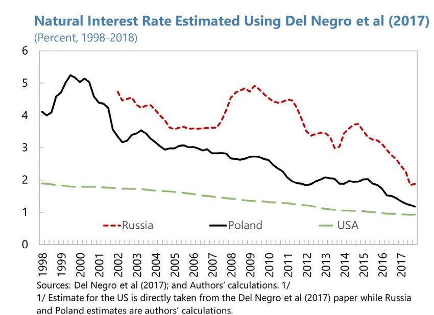
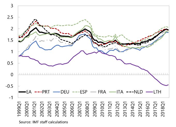
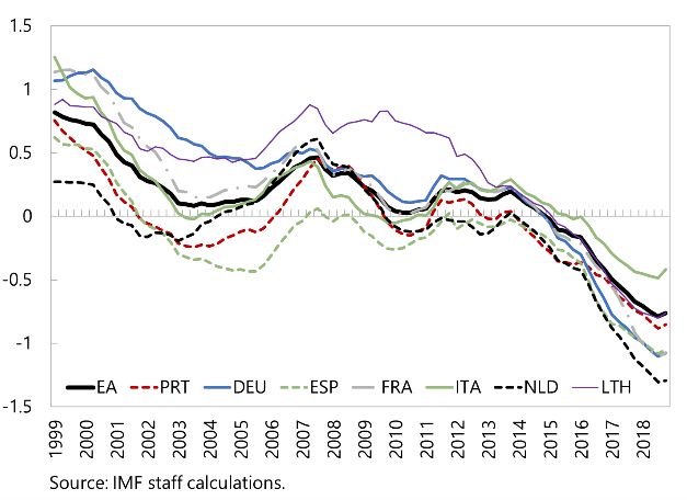
16

by using approaches that more directly look at interest rates to make inferences about r*. In
this logic, financial market data can be used to extract information about r*. Factor models
assume that the real interest rate should fluctuate around r* and that the difference between
them approaches zero as real and nominal shocks dissipate through time. Although these
models are agnostic about the economic drivers of natural rates, they can offer a useful set of
estimates that can be contrasted with those coming from more structural or semi-structural
models.

In this regard, the models proposed by Del Negro et al. (2017) and (2018) extract r* as a deep
trend from inflation, real short-term interest rates and real long rates using a Kalman filter
with Bayesian estimation techniques (see Annex V for details). The trend real short rate is
defined here as the measure of r*. Real variables are calculated from inflation data, nominal
short interest rates, and nominal long interest rates. The models further assume that that these
variables are cointegrated as follows:
 = ∗ + (8)

 3 = ∗ + ∗ + (9)
 10 
 = ∗ + ∗ + ∗ + (10)
 10 
where ∗ is trend inflation, 3 is the three-month T-bill rate, is the 10-year bond yield,
 ∗
 is the trend term premia, and , and are shocks (which can be persistent and
correlated with each other). The trend components are assumed to follow a random walk and
are subject to ‘white-noise’ shocks.

For the Euro Area, we estimate common factors on ∗ , ∗ and ∗ (the ‘Euro Area factors’),
as well country-specific trends, following Del Negro et al. (2018). The results show a clear
decline in r* for all Euro Area countries of around 2 percentage points, very similar to the
estimates from the L-W framework (Figure 4). In contrast with the estimates from the
previous section, however, our r* estimates from Factor models do not show a deep fall in
natural rates during crises periods, nor the subsequent modest rebound observed in L-W
estimates. In fact, the r* estimates from the Factor models are negative at around -1 percent
at mid-2019. This reflects the fact that real rates both at the long and the short end of the
yield curve remain near historic lows, together with the absence of structural features in these
type of models (as opposed to the L-W framework).

Compared to the L-W models, the co-movement of r* between countries is also much closer,
reflecting the explicit modeling of a common factor and the joint estimation procedure. In
this regard, Annex VI includes a comparison of our r* estimates using different
methodologies. There seems to be a broad movement towards similar r* levels rates since the
early 2000s, perhaps reflecting greater economic and financial integration following the
adoption of the euro, and at times some mispricing of risk, with interest rates in the south of
Europe very close to those in Germany. More recently, however, there has been some

17

divergence, which could reflect the fragmentation of financial markets since the GFC, a
clearer differentiation of country risk, and country-specific shocks.

In the case of emerging Europe, we use Del Negro et al. (2017) to estimate r*. Concretely,
our r* estimates are significantly higher than those for Euro Area countries, which is in line
with the results obtained using the L-W framework. Among other drivers, these results
reflect that real rates in emerging Europe are higher than those in the Euro Area throughout
the sample. In the case of Russia, r* falls from around 4 percent in the early 2000s to closer
to 2 percent by 2018. Within this broad decline, however, there is jump in 2008 (GFC) and
2014 (following sanctions), likely as a result of a spike in the risk premium. These peaks –
while not identical in timing or duration—are also found in the L-W model. In Poland, the
decline in r* was similarly in size—but was much steadier—reflecting perhaps smaller and/or
fewer shocks compared to Russia. This downward trend is also more pronounced than the
estimates derived from the L-W model. As a caveat, trend-cycle decompositions are less
suited for emerging economies as structural breaks are frequent. 16

 Figure 4: Natural Interest Rates Using Factor Models

 Natural Interest Rate Estimated using Common Factor Model
 (Percent, 1998-2018)
 1.5

 1

 0.5

 0

 -0.5

 -1

 EA PRT DEU ESP FRA ITA NLD LTH
 -1.5
 1999
 2000
 2001
 2002
 2003
 2004
 2005
 2006
 2007
 2008
 2009
 2010
 2011
 2012
 2013
 2014
 2015
 2016
 2017
 2018
 Source: Authors’ calculations.

Co-movement of r* Within the Euro Area

Countries within a currency union do not need to have the same natural rates or trend growth.
However, one can expect some co-movement of these series, especially as countries become
more integrated. We explore the time-varying interdependence of r* across Euro Area
countries in our sample via a multivariate Dynamic Conditional Correlation (DCC-) GARCH
model with one lag. We use our r* estimates and trend growth obtained from the application
of L-W model where is modeled as a function of certain external variables. As cautioned
in Holston et al. (2017), these series themselves are median estimates with a high level of
uncertainty, and thus, the interpretation of the coefficients and statistical significance of
statistical models should be taken with care. 17

16
 We did not run this model for Romania due to insufficient data.
17
 The model is estimated with Maximum Likelihood and Gaussian distributed errors.

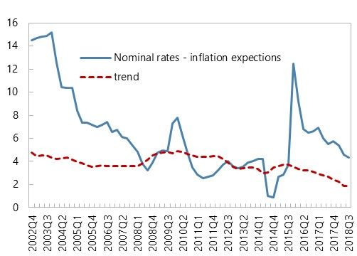
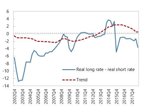
18

The covariance estimates are almost always positive, but strengthen or weaken over time,
indicating that r* across the Euro Area countries in our sample co-move, but not always to
the same degree (Figure 5). In periods of distress, such as the GFC and the sovereign debt
crisis, these estimates become more volatile. Covariances increase, but dispersion in bilateral
covariances also increase. For example, r* estimates for Spain and Portugal show much
stronger co-movement than between France and Germany during the 2011–14 period. Trend
growth estimates exhibit much lower and, in some cases, slightly negative covariances. Their
covariances are also higher and more dispersed during the sovereign debt crisis. The highest
covariances in trend growth are generally between Spain and three other countries (Portugal,
the Netherlands, and Italy) while Germany displays very low co-movement with
other countries.

 Figure 5. Co-movements in r* and g in the Euro Area
 Time-Varying Covariances of Estimates of Natural Rates Time-Varying Covariances of Trend Growth Estimates
 (Extended LW Model, 2001Q1-2019Q1) (Extended LW Model, 2001Q1-2019Q1)
 14 FRA v.s ITA FRA v.s DEU FRA v.s ITA FRA v.s DEU FRA v.s PRT FRA v.s NLD FRA v.s ESP
 FRA v.s PRT FRA v.s NLD 2.7 ITA v.s DEU ITA v.s PRT ITA v.s NLD ITA v.s ESP DEU v.s PRT
 12 FRA v.s ESP ITA v.s DEU
 ITA v.s PRT ITA v.s NLD DEU v.s NLD DEU v.s ESP PRT v.s NLD PRT v.s ESP NLD v.s ESP
 10 ITA v.s ESP DEU v.s PRT 2.2
 DEU v.s NLD DEU v.s ESP
 8 PRT v.s NLD PRT v.s ESP
 NLD v.s ESP 1.7

 6
 1.2
 4
 0.7
 2
 0.2
 0

 -2 -0.3
 2001Q1 2003Q2 2005Q3 2007Q4 2010Q1 2012Q2 2014Q3 2016Q4 2019Q1 2001Q1 2003Q2 2005Q3 2007Q4 2010Q1 2012Q2 2014Q3 2016Q4 2019Q1
 Sources: Using estimates from LW model, results of DCC-GARCH model, authors' calculations Sources: Using estimates from LW model, results of DCC-GARCH model, authors' calculations

What do Forward Interest Rates and the Term Structure say About the Future Path of r*?

Despite uncertainty, financial markets provide information on the direction that financial
markets “expect” r* to take in the future. If actual and natural rates of interest converge over
the medium term, as nominal and real shocks dissipate, financial market data can be used to
assess the market’s implicit “views” on the future path of r*. Market data also sheds light on
the terminal rate toward which policy interest rates may converge as some form of steady
state or equilibrium is approached. 18 To this end, we use two techniques to assess market’s
expectations about the future path of r*:

• Forward interest rates. The forward swap market on government debt gives an
 indication of the future path of short rates. Concretely, we use the three-month treasury
 bill, five-years ahead, as a proxy for the (nominal counterpart) of the neutral rate of
 interest. The relatively long period (five years) is chosen because it is judged likely to be

18
 For an exercise combining an arbitrage-free term structure model and a version of L-W, see Brand et
al (2020).

19

 enough for nominal rigidities not to bind. Inflation expectations are used to convert
 nominal rates into real rates.

• Term structure. We use a version of the Nelson-Siegal term structure model (Christensen
 et al, 2011) to fit the yield curve for a country’s government debt through time. This
 allows to separate the expected sequence of short-term rates from the term premium in a
 way that ensures that arbitrage conditions hold. From this, we derive the implied path of
 future nominal short rates (three-month treasury bill), consistent with this yield curve,
 and we use it as a proxy for the (nominal) natural rate in the future—specifically, five-
 years ahead. Inflation expectations are used again to convert nominal rates into real rates.

Figure 6 shows that for nearly
all Euro Area countries, as of Figure 6: Market Expectations of the Real Rate
June 2019, markets expected Percent
real interest rates to remain well 4.0
below zero for at least the
following five years. While 3.0
market expectations suggested 2.0
that real rates would increase 1.0
somewhat from the levels
observed as of mid-2019 0.0
(indicated by the blue dots), -1.0
their expected values were -2.0
below the range of r* estimates
presented in this paper. Thus, -3.0
while the analysis of previous DEU NLD LTU FRA PRT ESP ITA POL ROM RUS
sections suggested that real rates Forward rate Term structure Current r r* (three models)
should rise only moderately Source: Bloomberg, Haver, author calculations
 Note: Data on r, forwards and term structure are for June
(except in Italy) from the levels 2019. The estimates of r* are for the L-W model, the L-W
observed in mid-2019, markets model where z is modelled and the factor model
seemed to bet that r* and r were
unlikely to increase even that
much in the future, let alone move towards pre-GFC levels. This has important implications
for policy, considered below. In emerging Europe, market data should be viewed with more
caution given the likely higher liquidity and credit premia associated with these
instruments—this may explain part of the significant difference between our estimates of r*
and the path implied by markets. Nevertheless, in both Poland and Romania, market data
suggested a modest increase in real rates in the following years, but remaining well below
our estimates of r*. And in Russia, this analysis suggested that real rates would remain near
mid-2019 levels, and above r*, over the medium term.

20

 IV. POLICY IMPLICATIONS

Monetary Conditions

The estimate of r* compared to observed values of r provides information on the stance of
monetary policy. In countries that issue their own currencies, the r – r* gap provides a direct
assessment of the policy stance, while in countries that are members of a monetary union,
these gaps indicate how the common monetary policy is “felt” in individual member
countries, whose specific conditions will likely differ. In any case, the r – r* gap has a direct
bearing on the way the output gap evolves over time: the larger the positive (negative)
interest rate gap, the more contractionary (expansionary) is the monetary impulse.

Evidently, the complications surrounding the estimation of r* translate into uncertainty in the
assessment of the monetary stance. These challenges are more pressing in real time given
lags in data production and publication (Grigoli et al, 2015) and end-point issues. This
implies that estimates of r* need to be complemented by the analysis of other variables and
the use of judgment to produce a thorough assessment of monetary conditions. The
discussion below is based mostly on an examination during the sample period of the r – r*
gap, and thus should be taken as indicative only.

With these caveats, we estimate the monetary stance for the countries in our sample using r*
estimates derived from the application of the L-W framework when is modeled as a
function of economic variables. Real interest rates are calculated as the difference between
the Euro Area one-week inter-bank rate and five-year ahead inflation expectations. 19 While
inflation expectations in Euro Area countries differ, such differences are small, implying a
similar real short-term interest rate for all countries. Figure 7 shows that that prior to the
GFC, monetary conditions were loose, but began to tighten in 2007. Once the severity of the
GFC was fully realized, following Lehman’s failure, rates fell by over 3 percent within a
one-year period, and monetary conditions eased substantially in all countries. Given that the
ECB was close to the effective lower bound (ELB) by 2012, however, the room for further
policy cuts was limited, and the subsequent changes in the r – r* gap were driven largely by
the evolution of r*. Toward the end of the period under study, the analysis point to an
accommodative monetary conditions in all Euro Area countries, with the r – r* gap at around
-2 percent in 2019:Q1.

But there are important variations among Euro Area countries. For instance, Figure 7 shows
that in the case of France, the r – r* gap peaked by mid-2008 (increasing by over
2 percentage points from 2005 to 2008), and plummeted thereafter, falling below zero
exactly at the peak of the rate cycle (2008:Q3). That is, given France’s own r*, the common
policy was relatively soon having expansionary effects there. As the GFC moved into the

19
 This represents the closest approximation to the policy interest rate over this period. Prior to 2009, the inter-
bank rate moved closely with the ECB’s Main Refinancing Operation rate, but since then it has more closely
followed the Deposit Rate.

21

Euro Area, however, r* continued to decline markedly in the countries most affected by the
crisis, such as Portugal and Spain. In these countries, the monetary conditions, as reflected in
their interest rate gaps, were tight in mid-2008 and remained tighter for longer. This means
that the real interest rate fell for all countries, but such a decline was not equally effective in
creating expansionary conditions everywhere, as the output gaps and hence the need for
accommodation varied across countries (See Annex VI). Eventually, monetary conditions
turned expansionary even for these other countries.

Figure 7 combines information on interest rate gaps with information on output gaps and
inflation gaps (relative to target). This shows very crudely how well monetary conditions
aligned at different points with the inflation and output gaps, as in a simple Taylor rule. In
countries such as the Netherlands, where r* did not sink so low during the periods of stress,
the single Euro Area policy delivered appropriate monetary conditions, although towards the
end of the sample period conditions remained accommodative while the output gape was
turning positive. In other countries, with sharper movements in r*, the r – r* gap was unable
to deliver the accommodation that was desirable in view of their output gaps. This was the
case, for example, in Spain and Portugal during the euro area crisis. Between 2017 and 2019,
output gaps have narrowed (and likely closed) for many Euro Area countries, but the r- r*
gap continues to be negative for all. This is explained in part by the persistence of inflation
below 2 percent.

In the case of emerging Europe, monetary policy seems to have been broadly pro-cyclical in
Russia, and more so prior to the GFC. The description by the Central Bank of Russia of its
monetary policy stance in 2019 as “moderately tight” seems in line with the results we
obtain. In the case of Poland and Romania, the monetary policy stance seems to have been
broadly counter-cyclical during the global financial crisis and the taper tantrum, but has
become pro-cyclical in recent years.

An issue that deserves consideration is the impact of UMPs on monetary conditions. The
foregoing analysis implicitly assumes that monetary conditions are adequately described by
the estimated value of the r – r* gap. However, after hitting the ELB, the ECB started using
new instruments, which are not properly captured by the value of r in that gap. ‘Shadow’
interest rates (Krippner (2015), Wu and Xia (2016)), can be used to assess the stimulus
arising from asset purchases and forward guidance, actions that the ECB implemented once
policy rates reached the ELB. However, this is not as simple as replacing an estimated
shadow rate for an observed policy rate and comparing it to r*. Assessing the monetary
policy stance using shadow rates would require r* estimates that are constructed explicitly
considering UMPs, including a different transmission from the interest rate gap to the output
gap in the IS Curve. Estimated shadow rates would need to be an input into the calculation of
r* estimates that could then be used to obtain an alternative measure of the monetary stance
in the presence of UMPs. This is an interesting avenue for future research. Our conjecture is
that both the level of (shadow) r and r* are lower because of UMPs, but an assessment of the
impact of UMPs on the monetary stance would require further analysis.