A non-cooperative meta-modeling game for automated third-party calibrating, validating, and falsifying constitutive laws with parallelized ...
←
→
Page content transcription
If your browser does not render page correctly, please read the page content below
A non-cooperative meta-modeling game for automated
                                                  third-party calibrating, validating, and falsifying
                                               constitutive laws with parallelized adversarial attacks

                                                                   Kun Wang∗                WaiChing Sun†                 Qiang Du‡
arXiv:2004.09392v1 [eess.SP] 13 Apr 2020

                                                                                            April 21, 2020

                                                                                                 Abstract
                                                     The evaluation of constitutive models, especially for high-risk and high-regret engineering ap-
                                                 plications, requires efficient and rigorous third-party calibration, validation and falsification. While
                                                 there are numerous efforts to develop paradigms and standard procedures to validate models, dif-
                                                 ficulties may arise due to the sequential, manual and often biased nature of the commonly adopted
                                                 calibration and validation processes, thus slowing down data collections, hampering the progress
                                                 towards discovering new physics, increasing expenses and possibly leading to misinterpretations of
                                                 the credibility and application ranges of proposed models. This work attempts to introduce concepts
                                                 from game theory and machine learning techniques to overcome many of these existing difficulties.
                                                 We introduce an automated meta-modeling game where two competing AI agents systematically
                                                 generate experimental data to calibrate a given constitutive model and to explore its weakness, in
                                                 order to improve experiment design and model robustness through competition. The two agents
                                                 automatically search for the Nash equilibrium of the meta-modeling game in an adversarial rein-
                                                 forcement learning framework without human intervention. In particular, a protagonist agent seeks
                                                 to find the more effective ways to generate data for model calibrations, while an adversary agent
                                                 tries to find the most devastating test scenarios that expose the weaknesses of the constitutive model
                                                 calibrated by the protagonist. By capturing all possible design options of the laboratory experiments
                                                 into a single decision tree, we recast the design of experiments as a game of combinatorial moves
                                                 that can be resolved through deep reinforcement learning by the two competing players. Our adver-
                                                 sarial framework emulates idealized scientific collaborations and competitions among researchers
                                                 to achieve better understanding of the application range of the learned material laws and prevent
                                                 misinterpretations caused by conventional AI-based third-party validation. Numerical examples
                                                 are given to demonstrate the wide applicability of the proposed meta-modeling game with adver-
                                                 sarial attacks on both human-crafted constitutive models and machine learning models.

                                           1    Introduction and background
                                           As constitutive models that predict material responses become increasingly sophisticated and com-
                                           plex, the demands and difficulties for accurately calibrating and validating those constitutive laws
                                           also increase [Dafalias, 1984, Thacker et al., 2004, Borja, 2013, Liu et al., 2016, De Bellis et al., 2017,
                                              ∗ Fluid Dynamics and Solid Mechanics Group, Theoretical Division, Los Alamos National Laboratory, Los Alamos, NM

                                           87545. kunw@lanl.gov
                                              † Department of Civil Engineering and Engineering Mechanics, Columbia University, New York, NY 10027.

                                           wsun@columbia.edu (corresponding author)
                                              ‡ Department of Applied Physics and Applied Mathematics, and Data Science Institute, Columbia University, New York,

                                           NY 10027. qd2125@columbia.edu

                                                                                                     1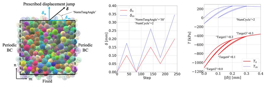
Bryant and Sun, 2018, Na et al., 2019a,b]. Engineering applications, particularly those involve high-
risk and high-regret decision-makings, require models to maintain robustness and accuracy in un-
foreseen scenarios using as little amount of necessary calibration data as possible. Quantifying the
reliability of a new constitutive law, however, is nontrivial. As many constitutive models are cali-
brated against limited amount and types of experimental data, identifying the reliable application
range of these constitutive laws beyond the loading paths used in the calibration could be challeng-
ing. While an apparent good match between predictions and calibration data can be easily achieved
by increasing the dimensionality of the parametric space of a given model, over-fitting may also jeop-
ardize the application of the learned models in the case where the predicted loading path bears little
resemblance to the calibration data [Wang et al., 2016, Gupta et al., 2019, Heider et al., 2020]. Using
such constitutive models therefore bears more risks for a third-party user who is unaware of the sensi-
tivity of material parameters on the stress predictions. Furthermore, the culture and the ecosystem of
the scientific communities often place a more significant focus on reporting the success of the material
models on limited cases. Yet, precise and thorough investigations on the weakness and shortcomings
of material models are important and often necessary, but they are less reported or documented in
the literature due to the lack of incentive [Pack et al., 2014, Boyce et al., 2016].
    Model calibration issues are critical not only for hand-crafted models but for many machine learn-
ing models and data-driven framework that either directly use experimental data to replace consti-
tutive laws Kirchdoerfer and Ortiz [2016, 2017], He and Chen [2019] or generate optimal response
surfaces via optimization problems [Bessa et al., 2017, Yang and Perdikaris, 2019, Zhu et al., 2019].
The recent trend of using black-box deep neural network (DNN) to generate constitutive laws has
made the reliability analysis even more crucial. At present, due to the lack of interpretability of
predictions generated by neural network, reliability of DNN generated constitutive laws is often as-
sessed through uncertainty quantification (UQ) [Yang and Perdikaris, 2019, Zhu et al., 2019]. UQ
can be conducted via different procedures, including Bayesian statistics, polynomial chaos expansion
and Monte Carlo sampling where one seeks to understand how probability distributions of the input
material parameters affect the outcomes of predictions, as often represented by some stress mea-
sures or performance metrics for solid mechanics applications. While UQ is a crucial step to ensure
the readiness of constitutive laws for engineering applications, a common challenge is to detect rare
events where a catastrophic loss of the prediction accuracy may occur in otherwise highly accurate
constitutive laws.
    The machine learning research community has been proposing methods to improve the inter-
polation and generalization capabilities, hence improving the predictive capability with exogenous
data as well as reducing the epistemic uncertainties of trained neural network models. For instance,
the active learning approaches (e.g. [Settles, 2009]), which is sometimes also referred as ”optimal
experimental design” [Olsson, 2009], introduce query strategies to choose what data to be gener-
ated to reduce generalization errors, balance exploration and exploitation and quantify uncertainties.
These approaches have repeatedly outperformed traditional ”passive learning” methods which in-
volve randomly gathering a large amount of training data. Active learning is widely investigated us-
ing different deep learning algorithms like CNNs and LSTMS [Sener and Savarese, 2017, Shen et al.,
2017]. There is also research on implementing Generative Adversarial Networks (GANs) into the ac-
tive learning framework [Zhu and Bento, 2017]. With the increasing interest in deep reinforcement
learning, researchers are trying to re-frame active learning as a reinforcement learning problem [Fang
et al., 2017]. Another recent study focuses on the ”semi-supervised learning” approaches [Zhu, 2005,
Verma et al., 2019, Berthelot et al., 2019], which take advantage of the structures of unlabeled input
data to enhance the ”interpolation consistency”, in addition to labeled training data. These recently
developed techniques have shown some degrees of successes for image recognition, natural language
processing, and therefore could potentially be helpful for mechanics problems.
    The calibration, validation and falsification of material models have issues similar to those dis-
cussed above. Moreover, experimental data are often expensive to get in both time and cost. Hence,
experimentalists would like to generate the least amount of data that can calibrate a constitutive
model with the highest reliability and can also identify its limitations. Traditionally the decisions on

                                                   2
which experiments to conduct are based on the human knowledge and experiences. We make an
effort here to use AI to assist the decision-makings of experimentalists, which will be the first of its
kind specifically targeting the automated design of data generation that can efficiently calibrate and
falsify a constitutive model.
     The major contribution of this paper is the introduction of a non-cooperative game that leads to
new optimized experimental designs that both improves the accuracy and robustness of the predic-
tions on unseen data, while at the same time exposing any potential weakness and shortcoming of a
constitutive law.
     We create a non-cooperative game in which a pair of agents are trained to emulate a form of ar-
tificial intelligence capable of improving their performance through trial and errors. The two agents
play against each other in a turn-based strategy game, according to their own agendas and pur-
poses respectively that serve to achieve opposite objectives. This setup constitutes a zero-sum game
in which each agent is rewarded by competing against the opponent. While the protagonist agent
learns to validate models by designing the experiments than enhance the model predictions, the ad-
versary agent learns how to undermine the protagonist agent by designing experiments that expose
the weakness of the models. The optimal game strategies for both players are explored by searching
for Nash equilibrium [Nash et al., 1950] of the games using deep reinforcement learning (DRL).
     With recent rapid development, DRL techniques have found unprecedented success in the last
decades on achieving superhuman intelligence and performance in playing increasingly complex
games: Atari [Mnih et al., 2013], board games [Silver et al., 2017b,a], Starcraft [Vinyals et al., 2019].
AlphaZero [Silver et al., 2017b] is also capable of learning the game strategies of our game without
human knowledge. By emulating the learning process of human learners through trial-and-error and
competition, the DRL process enables both AI agents to learn from their own successes and failures
but also through their competitions to master the tasks of calibrating and falsifying a constitutive
law. The knowledge gained from the competitions will help us understanding the relative rewards
of different experimental setup for validation and falsification mathematically represented by the
decision trees corresponding to the protagonist and adversary agents.
     The rest of the paper is organized as follows. We first describe the meta-modeling non-cooperative
game, including the method to recast the design of experiments into decision trees (Section 2). Follow-
ing this, we will introduce the detailed design of the calibration-falsification game for modeling the
competition between the AI experimental agent and the AI adversarial agent (Section 3). In Section 4,
we present the multi-agent reinforcement learning algorithms that enable us to find the optimal de-
cision for calibrating and falsifying constitutive laws. For numerical examples in Section 5, we report
the performances of the non-cooperative game on two classical elasto-plasticity models proposed by
human experts for bulk granular materials, and one neural networks model of traction-separation
law on granular interface.
     As for notations and symbols, bold-faced letters denote tensors (including vectors which are rank-
one tensors); the symbol ’·’ denotes a single contraction of adjacent indices of two tensors (e.g. a · b =
ai bi or c · d = cij d jk ); the symbol ‘:’ denotes a double contraction of adjacent indices of tensor of
rank two or higher ( e.g. C : ee = Cijkl ekl         e ); the symbol ‘⊗’ denotes a juxtaposition of two vectors

(e.g. a ⊗ b = ai b j ) or two symmetric second order tensors (e.g. (α ⊗ β)ijkl = αij β kl ). Moreover,
(α ⊕ β)ijkl = α jl β ik and (α β)ijkl = αil β jk . We also define identity tensors ( I )ij = δij , ( I 4 )ijkl = δik δjl ,
and ( I 4sym )ijkl = 21 (δik δjl + δil δkj ), where δij is the Kronecker delta.

2    AI-designed experiments: selecting paths in arborescences of de-
     cisions
Traditionally the decisions on which experiments to conduct are based a combination of intuition,
knowledge and experience from human. We make the first effort to use AI to assist the decision-
makings of experimentalists on how to get data that can efficiently calibrate and falsify a constitutive

                                                            3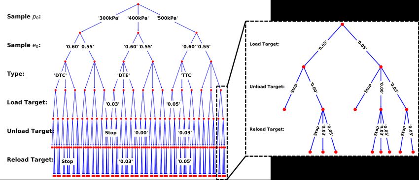
model. Our method differs from the existing machine learning techniques that we formulate the
experimentalist-model-critic environment as Markov games via decision-trees. In this game, the gen-
eration of calibration data is handled by a protagonist agent, once the model is calibrated, the testing
data are generated by an adversary agent to evaluate the forward prediction accuracy. The goal of the
adversary is to identify all application scenarios that the model will fail according to a user-defined
objective function (falsification). Hence the validation will be simultaneously achieved: the model is
valid within the calibration scenarios picked by protagonist and the testing scenarios that the adver-
sary has not picked. Practically, the model is safe to use unless the adversary ”warns” that the model
is at high risk. The formalization of decisions (or actions) as decision-trees, along with the communi-
cation mechanism designed in the game, enable AI agents to play this game competitively instead of
human players.
    Here we idealize the process of designing or planning an experiment as a sequence of decision
making among different available options. All the available options and choices in the design process
considered by the AI experimentalists (protagonist and adversary) are modeled by ”arborescences”
in graph theory with labeled vertices and edges. An arborescence is a rooted polytree in which, for
a single root vertex u and any other vertex v, there exists one unique directed path from u to v. A
polytree (or directed tree) is a directed graph whose underlying graph is a singly connected acyclic
graph. A brief review of the essential terminologies are given in Wang et al. [2019], and their detailed
definitions can be found in, for instance, Graham et al. [1989], West et al. [2001], Bang-Jensen and
Gutin [2008]. Mathematically, the arborescence for decision making (referred to as ”decision tree”
hereafter) can be expressed as an 8-tuple G = (LV , LE , V, E, s, t, nV , n E ) where V and E are the
sets of vertices and edges, LV and LE are the sets of labels for the vertices and edges, s : E → V
and t : E → V are the mappings that map each edge to its source vertex and its target vertex,
nV : V → LV and n E : E → LE are the mappings that give the vertices and edges their corresponding
labels (names) in LV and LE .
    The decision trees are constructed based on a hierarchical series of test conditions (e.g., category
of test, pressure level, target strain level) that an experimentalist needs to decide in order to design an
experiment on a material. Assuming that an experiment can be completely and uniquely defined by
an ordered list of selected test conditions tc = [tc1 , tc2 , tc3 , ..., tcn ], where NTC is the total number of
                                                                                                      m
test conditions. Each tci is selected from a finite set of choices TCi = {tc1i , tc2i , tc3i , ..., tci i }, where mi is
the number of choices for the ith test condition. For test conditions with inherently continuous design
variables, TCi can include preset discrete values. For example, the target strain for a loading can be
chosen from discrete values of 1%, 2%, 3%, etc. All design choices available to experimentalists are
represented by an ordered list of sets TC = [TC1 , TC2 , TC3 , ..., TCn ] with a hierarchical relationship
such that, if i < j, tci ∈ TCi must be selected prior to the selection of tc j ∈ TC j .
    After the construction of TC for experimentalists, a decision tree is built top-down from a root
node representing the ’Null’ state that no test condition is decided. The root node is split into m1
subnodes according to the first level of decisions TC1 . Each subnode is further split into m2 subnodes
according to the second level of decisions TC2 . The splitting process on the subnodes is carried out
recursively for all the NTC levels of decisions in TC. Finally, the down-most leaf nodes represent
all possible combinations of test conditions. The maximum number of possible configurations of
                              N
                            ∏i=TC1 mi , when all decisions across TCi are independent. The number of
experiments is Ntestmax =

possible experiments is reduced (Ntest < Ntest    max ) when restrictions are specified for the selections of

test conditions. E.g., the selection of tci ∈ TCi may prohibit the selections of certain choices tc j
in subsequent test conditions TC j , j > i. The experimentalists can choose multiple experiments by
taking multiple paths in the decision tree from the root node to the leaf nodes. The total number of
possible combination of paths, if the maximum allowed number of simultaneously chosen paths is
             max
            Npath
 max , is          k               k              Ntest !
Npath     ∑ k =1 C N test
                          , where CN test
                                          =   k!( Ntest −k )!
                                                                is the combination number.

Example for hierarchical test conditions and experimental decision tree. Consider a simple design of mechan-

                                                                  4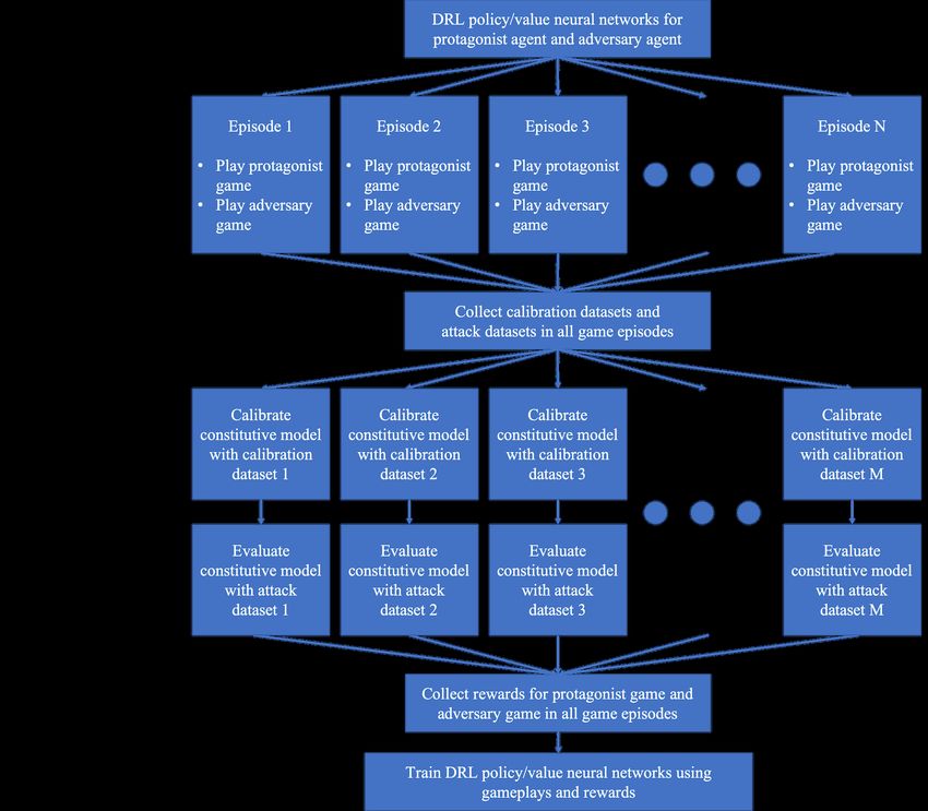
ical experiments for geomaterials, for which all choices are listed in

                                  TC = [’Sample’, ’Type’, ’Target’].                                 (1)

The first decision is to pick the initial geomaterial sample to test. Assuming that a sample is fully
characterized by its initial pressure p0 , a simple set of discrete sample choices is given as

                               TC1 = ’Sample’ = {’300kPa’, ’400kPa’}.                                (2)

The second test condition is the type of the experiment. The experiment can be either drained triaxial
compression test (’DTC’) or drained triaxial extension test (’DTE’). Then

                                   TC2 = ’Type’ = {’DTC’, ’DTE’}.                                    (3)

The third test condition to decide is the target strain magnitude for the loading. For example,

                                    TC3 = ’Target’ = {’1%’, ’3%’}.                                   (4)

After all three decisions are sequentially made (taking a path in the decision tree), the experiment
is completely determined by an ordered list, e.g., tc = [’300kPa’, ’DTE’, ’3%’]. It indicates that the
AI experimentalist decides to perform a monotonic drained triaxial extension test on a sample with
p0 = 300kPa until the axial strain reaches 3%.
    The decision tree G for the hierarchical design of geomaterial experiments specified by Equations
(1), (2), (3), (4) is shown in Fig. 1(a). The vertex sets and edge sets of the graph are

   V ={’Null’, ’300kPa’, ’400kPa’, ’300kPa DTC’, ’300kPa DTE’, ’400kPa DTC’, ’400kPa DTE’,
       ’300kPa DTC 1%’, ’300kPa DTC 3%’, ’300kPa DTE 1%’, ’300kPa DTE 3%’,
       ’400kPa DTC 1%’, ’400kPa DTC 3%’, ’400kPa DTE 1%’, ’400kPa DTE 3%’},
   E ={’Null’ → ’300kPa’, ’Null’ → ’400kPa’, ’300kPa’ → ’300kPa DTC’,
       ’300kPa’ → ’300kPa DTE’, ’400kPa’ → ’400kPa DTC’, ’400kPa’ → ’400kPa DTE’,
       ’300kPa DTC’ → ’300kPa DTC 1%’, ’300kPa DTC’ → ’300kPa DTC 3%’,                               (5)
       ’300kPa DTE’ → ’300kPa DTE 1%’, ’300kPa DTE’ → ’300kPa DTE 3%’,
       ’400kPa DTC’ → ’400kPa DTC 1%’, ’400kPa DTC’ → ’400kPa DTC 3%’,
       ’400kPa DTE’ → ’400kPa DTE 1%’, ’400kPa DTE’ → ’400kPa DTE 3%’},
 LV =V,
 LE ={’300kPa’, ’400kPa’, ’DTC’, ’DTE’, ’1%’, ’3%’}.
                             max = 2 ∗ 2 ∗ 2 = 8. If an experimentalist only collects data from one or
In this example, Ntest = Ntest
                         max
two experiments, i.e., Npath = 2, the total number of possible combinations is C81 + C82 = 36. Fig. 1(b)
presents two example paths with edge labels illustrating the hierarchical decisions on the test con-
ditions in order to arrive at the final experimental designs ’300kPa DTE 1%’ and ’400kPa DTC 3%’.

    In this section, we present two decision trees for the design of geomechanical experiments, one for
the bulk mechanical behavior of granular materials, another for the traction-separation behaviour of
granular interfaces. We later study the intelligence of the reinforcement-learning-based experimen-
talists (protagonist and adversary) on these decision trees in Section 5.

2.1   Decision tree for AI-guided experimentation on bulk granular materials
This section defines a representative decision tree for the AI-guided experimentation on bulk geoma-
terials. The hierarchical series of test conditions includes six elements, TC = [TC1 , TC2 , TC3 , TC4 ,

                                                   5
(a) Decision tree with labels of vertices and edges (b) Example of paths in the decision tree, the selected tests are
’300kPa DTE 1%’ and ’400kPa DTC 3%’
Figure 1: Decision tree for a simple experimental design for geomaterials (Eq. (1), (2), (3), (4)).
TC5 , TC6 ], such that the AI experimentalists can choose isotropic granular samples of different ini-
tial pressure p0 and initial void ratio e0 , perform different drained triaxial tests, and design different
loading-unloading-reloading paths.
The choices for each test conditions are shown in Table 1, represented by decision labels. The
decision labels for the test types TC3 are defined as follows,
1. ’DTC’: drained conventional triaxial compression test (ė11 < 0, σ̇22 = σ̇33 = σ̇12 = σ̇23 = σ̇13 =
0),
2. ’DTE’: drained conventional triaxial extension test (ė11 > 0, σ̇22 = σ̇33 = σ̇12 = σ̇23 = σ̇13 = 0),
σ22 −σ33
3. ’TTC’: drained true triaxial test with b = 0.5 (ė11 < 0, b = σ11 −σ33 = const, σ̇33 = σ̇12 = σ̇23 =
σ̇13 = 0),
with the loading conditions represented by constraints on the components of the stress rate and strain
rate tensors
ė11 ė12 ė13 σ̇11 σ̇12 σ̇13
ė = ė22 ė23 , σ̇ = σ̇22 σ̇23 . (6)
sym ė33 sym σ̇33
Since ’DTC’ and ’DTE’ are special cases of true triaxial tests, the choices {’DTC’, ’DTE’, ’TTC’} for
−σ33
TC3 are equivalent to choosing the value of b = σσ22 − from {’0.0’, ’1.0’, ’0.5’}, respectively [Ro-
11 σ33
driguez and Lade, 2013].
The decision labels ’NaN’ in TC5 and TC6 indicate that the unloading or reloading is not acti-
vated. This design enables the freedom of generating monotonic loading paths (e.g., ’5% NaN NaN’),
loading-unloading paths (e.g., ’5% 0% NaN’) and loading-unloading-reloading paths (e.g., ’5% 0% 3%’).
There are restrictions in choosing the strain targets. The experimentalist picks the loading target in
TC4 first and the unloading target in TC5 must be, if not ’NaN’ (stop the experiment), smaller than
the loading strain. Then the reloading target in TC6 must be, if not ’NaN’, larger than the unloading
strain.
6
TC Test Conditions                   Choices
                  TC1 = ’Sample p0 ’                   {’300kPa’, ’400kPa’, ’500kPa’}
                  TC2 = ’Sample e0 ’                   {’0.60’, ’0.55’}
                  TC3 = ’Type’                         {’DTC’, ’DTE’, ’TTC’}
                  TC4 = ’Load Target’                  {’3%’, ’5%’}
                  TC5 = ’Unload Target’                {’NaN’, ’0%’, ’3%’}
                  TC6 = ’Reload Target’                {’NaN’, ’3%’, ’5%’}

      Table 1: Choices of test conditions for AI-guided experimentation on bulk granular materials.

    The corresponding decision tree is shown in Fig. 2. The subtree concerning the restricted decision-
making in TC4 , TC5 and TC6 is also detailed in the figure. The total number of experimental designs
(which equals to the number of leaf nodes in the tree) is Ntest = 180. Fig. 3 provides the experimental
settings on DEM (discrete element methods) numerical specimens and data from one example of the
experiments. The total number of experimental data combinations increases significantly when the
                                          max increases. The combination number equals to C1
maximum allowed simultaneous paths Npath                                                          180 =
           max = 1, equals to C1 + C2                 max                  1      2      3
180 when Npath                 180  180 = 16290 when Npath = 2, equals to C180 + C180 + C180 =
               max = 3, etc.
972150 when Npath

Figure 2: Decision tree for AI-guided drained true triaxial tests on bulk granular materials. Due to
the complexity of the graph, the vertex labels are omitted, and only a few edge labels are shown. See
Fig. 1 for exhaustive vertex and edge labels in a simple decision tree example.

2.2     Decision tree for AI-guided experimentation on granular interfaces
This section defines a representative decision tree for the AI-guided experimentation on granular in-
terfaces. The hierarchical series of test conditions includes six elements, TC = [TC1 , TC2 , TC3 , TC4 ,
TC5 , TC6 ], such that the AI experimentalists can choose the direction of the prescribed displace-
ment jump, the number of loading cycles, and different target displacement values to design complex
loading paths.
    The choices for each test conditions are shown in Table 2, represented by decision labels. ’Norm-
TangAngle’ represents the angle between the displacement jump vector and the tangential direction
vector, the corresponding values in the Choices column are in units of degree. ’NumCycle’ represents

                                                   7
Figure 3: Experimental settings of drained true triaxial tests on numerical specimen of bulk granular
materials using DEM (discrete element methods). The test conditions for the AI experimentalist are
presented in Table 1. As an example, the differential stress data and volumetric strain data obtained
from a test designed by the decision tree path ’300kPa’ → ’0.55’ → ’DTC’ → ’3%’ → ’0%’ → ’5%’ are
presented.

the number of loading-unloading cycles. The conditions ’Target1’, ’Target2’, ’Target3’, ’Target4’ repre-
sent the target displacement jump magnitudes along the loading-unloading cycles, the corresponding
values in the Choices column are in units of millimeters. Regardless of the loading-unloading cycles,
the final displacement jump reaches the magnitude of 0.4 mm. The decision label ’NaN’ indicates that
the unloading or reloading is not activated. For example, ’NumCycle’=’0’ means a monotonic loading
to 0.4 mm, hence all the target conditions should adopt the values of ’NaN’; ’NumCycle’=’1’ means a
loading-unloading-reloading path to 0.4 mm, hence ’Target1’ (loading target) and ’Target2’(unloading
target) can adopt values within ’0.0’, ’0.1’, ’0.2’, ’0.3’, while ’Target3’ and ’Target4’ should be ’NaN’s.

       TC Test Conditions                   Choices
       TC1 = ’NormTangAngle’                {’0’, ’15’, ’30’, ’45’,   ’60’, ’75’}
       TC2 = ’NumCycle’                     {’0’, ’1’, ’2’}
       TC3 = ’Target1’                      {’NaN’, ’0.1’, ’0.2’,     ’0.3’}
       TC4 = ’Target2’                      {’NaN’, ’0.0’, ’0.1’,     ’0.2’}
       TC5 = ’Target3’                      {’NaN’, ’0.1’, ’0.2’,     ’0.3’}
       TC6 = ’Target4’                      {’NaN’, ’0.0’, ’0.1’,     ’0.2’}

      Table 2: Choices of test conditions for AI-guided experimentation on granular interfaces.

    The corresponding decision tree is shown in Fig. 4. The total number of experimental designs
(which equals to the number of leaf nodes in the tree) is Ntest = 228. Fig. 5 provides the experimental
settings on DEM (discrete element methods) numerical specimens and data from one example of the
experiments. The total number of experimental data combinations, for example, equals to C228         1 +
  2 + C3                        max
C228     228 ≈ 1.97e6 when Npath = 3. Such number is already impractical for human to find the
optimal data sets for calibration and falsification by trial and error. For high efficiency, the decisions
in performing experiments should be guided by experienced experts or, in this paper, reinforcement-
learning-based AI.

                                                     8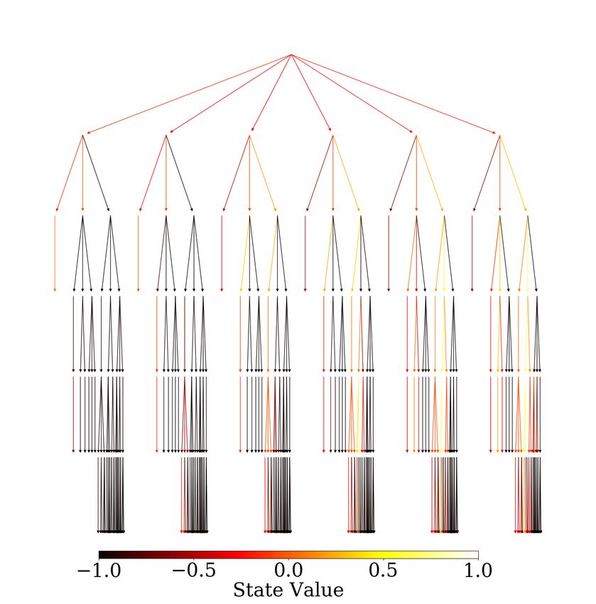
Figure 4: Decision tree for AI-guided displacement-driven mixed-mode shear tests on granular inter-
faces. Due to the complexity of the graph, the vertex labels are omitted, and only a few edge labels
are shown.
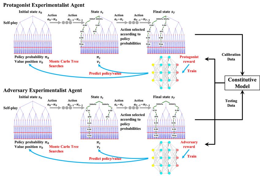
Figure 5: Experimental settings of displacement-driven mixed-mode shear tests on numerical spec-
imen of granular interfaces using DEM (discrete element methods). The test conditions for the AI
experimentalist are presented in Table 2. As an example, the loading path and traction in normal
and tangential directions obtained from a test designed by the decision tree path ’30’ → ’2’ → ’0.2’
→ ’0.0’ → ’0.3’ → ’0.1’ are presented. Regardless of the designed loading-unloading cycles, the final
displacement jump reaches the magnitude of 0.4 mm.
3 Multi-agent non-cooperative game for model calibration/falsifi-
cation with adversarial attacks
This section presents the design of a data acquisition game for both AI experimentalists (protagonist
and adversary) to play, based on the decision trees defined in Section 2 involving the common actions
9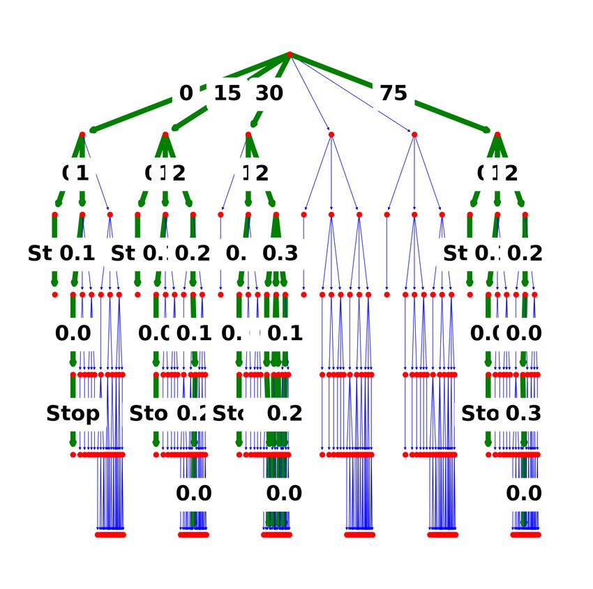
in testing the mechanical properties of geomaterials. The goal of this game is to enable the protagonist
agent to find the optimal design of experiments that best calibrate a constitutive law, while having
the adversary agent designs a counterpart set of experiments that expose the weakness of the models
in the same decision tree that represents the application range. For simplicity, we assume that all
experiments conducted by both agents are fully reproducible and free of noise. We will introduce a
more comprehensive treatment for more general situations in which the bias and sensitivity of the
data as well as the possibility of erroneous and even fabricated data are considered in future. Such a
treatment is, nevertheless out of the scope of this work.
    Multi-agent multi-objective Markov games [Littman, 1994] have been widely studied and applied
in robotics [Pinto et al., 2017], traffic control [Wiering, 2000], social dilemmas [Leibo et al., 2017], etc.
In our previous work, Wang et al. [2019], our focus was on designing agents that have different ac-
tions and states but share the same goal. In this work, our new innovation is on designing a zero-sum
game in which the agents are competing against each other for a pair of opposite goals. While the
reinforcement learning may lead to improved game play through repeated trial-and-error, the non-
cooperative nature of this new game will force the protagonist to act differently in response to the
weakness exposed by the adversary. This treatment therefore may lead to a more robust and regu-
larized model. In this work, the protagonist and the adversary are given the exact same action space
mathematically characterized as a decision tree. While a non-cooperative game with non-symmetric
action spaces can enjoy great performance as demonstrated in some of the OpenAI systems [Pinto
et al., 2017], such an extension is out of the scope of this study and will be considered in the future.

3.1    Non-cooperative calibration/falsification game involving protagonist and ad-
       versary
We follow the general setup in Pinto et al. [2017] to create a two-player Markov game with competing
objectives to calibrate and falsify a constitutive model. Both calibration and falsification are idealized
as procedures that involves sequences of actions taken to maximize (in the case of calibration) and
minimize (in the case of the falsification) a metric that assesses the prediction accuracy and robustness.
       Consider the Markov decision process (MDP) in this game expressed as a tuple (S , A p , A a , P , r p , r a , s0 )
where S is the set of game states and s0 is the initial state distribution. A p is the set of actions
taken by the protagonist in charge of generating the experimental data to calibrate a given material
model. A a is the set of actions taken by the adversary in charge of falsifying the material model.
P : S × A p × A a × S → R is the transition probability density. r p : S × A p × A a → R and
r a : S × A p × A a → R are the rewards of protagonist and adversary, respectively. If r p = r a ,
the game is fully cooperative. If r p = −r a , the game is zero-sum competitive. At the current
state s of the game, if the protagonist is taking action a p sampled from a stochastic policy µ p and
the adversary is taking action a a sampled from a stochastic policy µ a , the reward functions are
  µ p ,µ a                                                            µ ,µ
rp         = Ea p ∼µ p (·|s),aa ∼µa (·|s) [r p (s, a p , a a )] and r a p a = Ea p ∼µ p (·|s),aa ∼µa (·|s) [r a (s, a p , a a )].
       In this work, all the possible actions of the protagonist and the adversary agent are mathematically
represented by decision trees (Section 2). The protagonist first selects one or more paths in its own
tree which provide the detailed experimental setups to generate calibration data for the material
model, then the adversary selects one or more paths in its own tree (identical to the protagonist’s
tree) to generate test data for the calibrated model, aiming to find the worst prediction scenarios. The
rewards are based on the prediction accuracy measures SCORE of the constitutive model against data.
This measure of ’win’ or ’lose’ is only available when the game is terminated, similar to Chess and Go
[Silver et al., 2017b,a], thus the final rewards are back-propagated to inform all intermediate rewards
r p (s, a p , a a ) and r a (s, a p , a a ). r p is defined to encourage the increase of SCORE of model calibrations,
while r a is defined to favor the decrease of SCORE of forward predictions. In this setting, the game is
non-cooperative, and generally not zero-sum.

                                                            10
3.2 Components of the game for the experimentalist agents
The agent-environment interactive system (game) for the experimentalist agents consists of the game
environment, game states, game actions, game rules, and game rewards [Bonabeau, 2002, Wang and
Sun, 2019] (Fig. 6). These key ingredients are detailed as follows.
Figure 6: Key ingredients (environment, agents, states, actions, rules, and rewards) of the two-player
non-cooperative agent-environment interactive system (game) for the experimentalist agents.
Game Environment consists of the geomaterial samples, the constitutive model for performance
evaluation, and the experimental decision trees. The samples in this game are representative volume
elements (RVEs) of virtual granular assemblies modeled by the discrete element method (DEM) (e.g.,
Fig. 3, Fig. 5). The preparation of such DEM RVEs are detailed in the numerical examples. The con-
stitutive model can be given by the modeler agent in a meta-modeling game [Wang and Sun, 2019,
Wang et al., 2019]. In this paper, we focus on the interactive learning of data acquisition strategies for
a certain constitutive model of interest. Three-agent protagonist-modeler-adversary reinforcement
learning games is out of the scope of the current study. The protagonist and adversary agents de-
termine the experiments on the RVEs in order to collect data for model parameter identification and
testing the forward prediction accuracy of the constitutive model, respectively, via taking paths in
their own decision trees (e.g., Fig. 1, Fig. 2, Fig. 4).
Game State For the convenience of deep reinforcement learning using policy/value neural net-
works, we use a 2D array s(2) to concisely represent the paths that the protagonist or adversary has
selected in the experimental decision tree. The mapping from the set of the 2D arrays to the set of
path combinations in the decision tree is injective. The array has a row size of Npath max and a column
size of NTC . Each row represents one path in the decision tree from the root node to a leaf node, i.e.,
a complete design of one experiment. The number of allowed experiments is restricted by the row
max , which is defined by the user. Each array entry in the N
size Npath TC columns represents the selected
decision label of each test condition in TC. The entry a (integer) in the jth row and ith column indi-
cates that the ath decision label in the set TCi is selected for the jth experiment. Before the decision
max , with its kth entry indicating whether
tree selections, the agent first decide a 1D array s(1) of size Npath
11the agent decides to take a new path in the decision tree (perform an another experiment) after the
current kth experiment is done. A value of 1 indicates continuation and 2 indicates stop. The total
state s of the game combines s(1) and s(2) , with s(2) flattened to a 1D array of size Npath max ∗ N
TC and
then input into the policy/value neural networks for policy evaluations. Initially, all entries in the
arrays are 0, indicating no decisions has been made.
Game Action The AI agent works on the game state arrays by changing the initial zero entries into
integers representing the decision labels. The agent firstly selects 1 for continuation or selects 2 for
stop in s(1) , in the left-to-right order. The agent then works on s(2) in the left-to-right then top-to-
bottom order. Suppose that the first zero element of the current state array s(2) is in the jth row and
ith column, the agent will select an integer 1 ≤ a ≤ mi (number of choices) to choose a decision label
in TCi . The size of the action space is Naction = maxi∈[1,NTC ] mi .
Game Rule The AI agents are restricted to follow existing edges in the constructed decision tree,
which has already incorporated decision limitations such as the choices of loading/unloading/reload-
ing strain targets. The game rules are reflected by a list of Naction binaries Legal Actions(s) = [ii1 , ii2 , ..., ii Naction ]
at the current state s. If the ath decision is allowed, the ath entry is 1. Otherwise, the entry is 0. Figure
7 provides an example of the mathematical representations of the game states, actions and rules of
the decision tree game.
Figure 7: Example of the current st and next st+1 game states describing the selected edges in the
decision tree, action by the agent at to ”advance” in the decision tree, and the legal actions at the
max = 2.
current state, with Npath
Game Reward The rewards from the game environment to the experimentalists should consider
the performance of a given constitutive model on calibration data and testing data. After the decision
of experiments by the protagonist, these experiments are performed on material samples to collect
data. Then the constitutive model is calibrated with these data, and the accuracy is evaluated by
a model score SCOREprotagonist . After the decision of experiments by the adversary, the calibrated
constitutive model gives forward predictions on these testing data. The accuracy is evaluated by
a model score SCOREadversary . +SCOREprotagonist is returned to the protagonist to inform its game
reward, while −SCOREadversary is returned to the adversary. This adversary attack reward system is
the key to ensure that the protagonist generates calibration data to maximize the prediction strength
of the constitutive model, while the adversary tries to explore the weakness of the model.
123.3 Evaluation of model scores and game rewards
The accuracy of model calibrations and forward predictions are quantified by calculating the discrep-
data Ndata model Ndata
ancy between the vector of data points [Y i ] i =1 and the vector of predicted values [Y i ] i =1
j j
under the same experimental conditions. For both data points and predictions, Y i = S j (Yi ), where Yi
is the data that falls into the jth category of output features (quantities of interest, such as deviatoric
stress q and void ratio e). S j is the scaling operator (standardization, min-max scaling, ...) for the jth
output feature.
model N
The predictions [Y i ]i=data
1 come from a given constitutive model that is calibrated with data gen-
erated by the protagonist. In this work, for elasto-plastic models, the nonlinear least-squares solver
”NL2SOL” in Dakota software [Adams et al., 2014] is used to find the optimal parameter values. The
initial guess, upper and lower bounds of each parameter are given by domain experts’ knowledge
and preliminary estimations. For models of artificial neural networks, parameters are tuned by back-
propagation algorithms using Tensorflow [Abadi et al., 2015]. In both cases, the optimal material
parameters minimize the scaled mean squared error objective function
Ndata
1 model data 2
scaled MSE =
Ndata ∑ (Y i − Yi ) . (7)
i =1
The model scores measuring the prediction accuracy are based on the modified Nash-Sutcliffe
efficiency index [Nash and Sutcliffe, 1970, Krause et al., 2005],
N data model j
j ∑i=data
1 |Y i − Yi |
ENS = 1 − data data
∈ (−∞, 1.0]. (8)
N
∑i=data
1 |Y i − mean(Y )| j
When j = 2, it recovers the conventional Nash-Sutcliffe efficiency index. Here we adopt j = 1, and
min(max( E1NS , Emin max min max
NS ), E NS ) − 0.5 ∗ ( E NS + E NS )
SCOREprotagonist or adversary = 2 ∗ , (9)
Emax min
NS − E NS
where Emax min
NS and E NS are maximum and minimum cutoff values of the modified Nash-Sutcliffe effi-
ciency index, SCORE ∈ [−1.0, 1.0].
The game reward returned to the protagonist can consider both the calibration accuracy and the
forward prediction accuracy, by including an exponential decay term:
Rewardprotagonist = −1 + (SCOREprotagonist + 1) ∗ exp [−αSCORE ∗ max( Emin 1
NS − min({ E NS }), 0)]. (10)
where min({ E1NS }) is the minimum N-S index observed in the gameplay history, αSCORE is a user-
defined decay coefficient. When min({ E1NS }) < Emin
NS , the decay term starts to drop the reward of the
protagonist, otherwise Rewardprotagonist = +SCOREprotagonist . On the other hand, the game reward
returned to the adversary is
Rewardadversary = −SCOREadversary . (11)
Since the adversary is rewarded at the expense of the protagonist’s failure, it is progressively learning
to create increasingly devastating experimental design to falsify the model, thus forcing the protag-
onist to calibrate material models that are robust to any disturbances created by the adversary. In
this work, we refer to the move of the protagonist as calibration or defense, while the move of the
adversary as falsification or attack.
134 Parallel reinforcement learning algorithm for the non-cooperative
experimental/adversarial game
In the language of game theory, the meta-modeling game defined in the previous section is cate-
gorized as non-cooperative, asymmetric (the payoff of a particular strategy depends on whether
protagonist or adversary is playing), non-zero-sum, sequential (the adversary is aware of the pro-
tagonist’s strategy in order to attack accordingly), imperfect information (the protagonist does not
know how the adversary will attack). Let (M, R) be a representation of this two-player (denoted by
subscripts p and a) non-cooperative game, with M = M p × M a the set of strategy profiles. R(µ) =
(R p (µ), R a (µ)) is the payoff (final reward) function evaluated at a strategy profile µ = (µ p , µ a ) ∈ M.
A strategy profile µ∗ is a Nash equilibrium if no unilateral change in µ∗ by any player is more prof-
itable for that player, i.e.,
∀µ p ∈ M p , R p ((µ∗p , µ∗a )) ≥ R p ((µ p , µ∗a ))
(
. (12)
∀µ a ∈ M a , R a ((µ∗p , µ∗a )) ≥ R a ((µ∗p , µ a ))
The existence of at least one such equilibrium point is proven by Nash et al. [1950].
Solving the optimization problem directly to find the Nash equilibria strategies for this complex
game is prohibitive [Perolat et al., 2015]. Instead, deep reinforcement learning (DRL) algorithm is
employed. In this technique the strategy of each player (µ p or µ a ) is parameterized by an artificial
neural network f θ that takes in the description of the current state s of the game and outputs a policy
vector p with each component representing the probability of taking actions from state s, as well as a
scalar v for estimating the expected reward of the game from state s, i.e.,
( p, v) = f θ (s). (13)
These policy/value networks provide guidance in learning optimal strategies of both protagonist and
adversary in order to maximize the final game rewards. The learning is completely free of human
interventions after the complete game settings. This tactic is considered one of the key ideas leading
to the major breakthrough in AI playing the game of Go (AlphaGo Zero) [Silver et al., 2017b], Chess
and shogi (Alpha Zero) [Silver et al., 2017a] and many other games. In Wang and Sun [2019], the key
ingredients (policy/value network, upper confidence bound for Q-value, Monte Carlo Tree Search)
of the DRL technique are detailed and applied to a meta-modeling game for modeler agent only,
focusing on finding the optimal topology of physical relations from fixed training/testing datasets.
Since DRL needs to figure out the optimal strategies for both agents, the algorithm is extended to
multi-agent multi-objective DRL [Tan, 1993, Foerster et al., 2016, Tampuu et al., 2017]. The AI for
protagonist and adversary are improved simultaneously during the self-plays of the entire meta-
modeling game, according to the individual rewards they receive from the game environment and
the communications between themselves (Figure 8).
The pseudocode of the reinforcement learning algorithm to play the non-cooperative game is
presented in Algorithm 1. This is an extension of the algorithm in [Wang and Sun, 2019]. As demon-
strated in Algorithm 1, each complete DRL procedure involves numIters number of training iterations
and one final iteration for generating the converged selected paths in decision trees. Each iteration in-
volves numEpisodes number of game episodes that construct the training example set trainExamples
Protagonist Adversary
for the training of the policy/value networks f θ and f θ . For decision makings in each
game episode, the action probabilities are estimated from numMCTSSims runs of MCTS simulations.
The state values v can be equal to the continuous reward functions (10), (11) to train the poli-
cy/value neural networks. To further improve the convergence rate of the DRL algorithm, we pro-
pose an empirical method to train the networks with binary state values (1 or -1) post-processed
from the reward values, which is similar to the concept of ”win” (1) and ”lose” (-1) in the game
of Chess. Consider the set of rewards {Rewardprotagonist }i of the numEpisodes games played in
14Figure 8: Two-player adversarial reinforcement learning for generating optimal strategies to automate
the calibration and falsification of a constitutive model.
the ith DRL iteration. The maximum reward encountered from Iteration 0 to the current Itera-
tion k, is Rmax
p = maxi∈[0,k] (max({Rewardprotagonist }i )). A minimum reward is chosen as Rmin p =
range
maxi∈[0,k] (min({Rewardprotagonist }i )). A reward range in Iteration k is R p = Rmaxp − R min . A strat-
p
range
egy µ p is considered as a ”win” (v = 1) when its reward Rewardprotagonist ≥ Rmax p − R p ∗ αrange ,
max range
while it is a ”lose” (v = −1) when Rewardprotagonist < R p − R p ∗ αrange . αrange is a user-defined
coefficient which influences the degree of ”exploration and exploitation” of the AI agents. Similarly,
µp µp
for the adversary agent, Rmax min
aµ p = mini ∈[0,k ] (max({−Rewardadversary }i )), R aµ p = mini ∈[0,k ] (min({−Rewardadversary }i ))
range
and R aµ p = Rmax min
aµ p − R aµ p are collected for each protagonist strategy µ p . Then an attack strat-
µp
egy µ a corresponding to µ p is considered as a ”win” (v = 1) when its reward −Rewardadversary ≤
range µp range
Rmin min
aµ p + R aµ p ∗ αrange , while it is a ”lose” (v = −1) when −Rewardadversary > R aµ p + R aµ p ∗ αrange .
The training examples for the policy/value neural networks are limited to the gameplays in the DRL
iterations i ∈ [max(k − ilookback , 0), k], where ilookback is a user-defined hyperparameter controlling the
degree of ”forget” of the AI agents.
Another new contribution to the DRL framework is that we improve the computational efficiency
of DRL by executing the mutually independent gameplays and reward evaluations in a parallel man-
ner, instead of serial executions as in previous works [Wang and Sun, 2018, 2019, Wang et al., 2019].
We use the parallel python library ”Ray” [Moritz et al., 2018] for its simplicity and speed in building
and running distributed applications. The new workflow of parallel playing of game episodes in each
training iteration for DRL is illustrated in Figure 9.
15Algorithm 1 Self-play reinforcement learning of the non-cooperative meta-modeling game
Require: The definitions of the non-cooperative meta-modeling game: game environment, game
states, game actions, game rules, game rewards (Sections 3).
Protagonist Adversary
1: Initialize the policy/value networks f θ and f θ . For fresh learning, the networks
are randomly initialized. For transfer learning, load pre-trained networks instead.
2: Initialize empty sets of the training examples for both protagonist and adversary
trainExamplesProtagonist ← [], trainExamplesadversary ← [].
3: for i in [0,..., numIters − 1] do
4: for j in [0,..., numEpisodes − 1] do
5: Initialize the starting game state s.
6: for player in [Protagonist, Adversary] do
7: Initialize empty tree of the Monte Carlo Tree search (MCTS), set the temperature pa-
rameter τtrain for ”exploration and exploitation”.
8: while True do
9: Check for all legal actions at current state s according to the game rules.
10: Get the action probabilities π (s, ·) for all legal actions by performing
numMCTSSims times of MCTS simulations.
11: Sample action a from the probabilities π (s, ·)
12: Modify the current game state to a new state s by taking the action a.
13: if s is the end state of the game of player then
14: Evaluate the score of the selected paths in the decision tree.
15: Evaluate the reward r of this gameplay according to the score.
16: Break.
17: Append the gameplay history [s, a, π (s, ·), r ] to trainExamples player .
Protagonist Adversary
18: Train the policy/value networks f θ and f θ with trainExamplesProtagonist and
trainExamplesAdversary .
Protagonist Adversary
19: Use the final trained networks f θ and f θ in MCTS with temperature parameter
τtest for one more iteration of ”competitive gameplays” to generate the final converged selected
experiments.
20: Exit
16Figure 9: Workflow of parallel gameplays and reward evaluations in DRL.
5 Automated calibration and falsification experiments
We demonstrate the applications of the non-cooperative game for automated calibration and falsifica-
tion on three types of constitutive models. The material samples are representative volume elements
(RVEs) of densely-packed spherical DEM particles. The decision-tree-based experiments are per-
formed via numerical simulations on these samples. The preparation and experiments of the samples
are detailed in Appendix A. The three constitutive models studied in this paper are Drucker-Prager
model [Tu et al., 2009], SANISAND model [Dafalias and Manzari, 2004], and data-driven traction-
separation model [Wang and Sun, 2018]. Their formulations are detailed in Appendix B. The re-
sults shown in this section are representatives of the AI agents’ performances, since the policy/value
networks are randomly initialized and the MCTS simulations involve samplings from action proba-
bilities. The gameplays during DRL iterations may vary, but similar convergence performances are
expected for different executions of the algorithm. Furthermore, the material calibration procedures,
such as the initial guesses in Dakota and the hyperparameters in training of the neural networks, may
affect the game scores and the converged Nash equilibrium points. Finally, since simplifications and
assumptions are involved in the DEM samples, their mechanical properties differ from real-world
geo-materials. The conclusions of the three investigated constitutive models are only on these artifi-
cial and numerical samples. However, the same DRL algorithm is also applicable for real materials,
17when the actions of the AI experimentalists can be programmed in laboratory instruments.
The policy/value networks f θ are deel neural network in charge of updating the Q table that deter-
mines the optimal strategies. The design of the policy/value networks are identical for both agents in
this paper. Both of them consist of one input layer of the game state s, two densely connected hidden
layers, and two output layers for the action probabilities p and the state value v, respectively. Each
hidden layer contains 256 artificial neurons, followed by Batch Normalization, ReLU activation and
Dropout. The dropout layer is a popular regularization mechanism designed to reduce overfitting
and improve generalization errors in deep neural network (cf. Srivastava et al. [2014]). The dropout
rate is 0.5 for the protagonist and 0.25 for the adversary. These different dropout rates are used such
that the higher dropout rate for the protagonist will motivate the protagonist to calibrate the Drucker-
Prager model with less generalization errors, while the smaller dropout rate will help the adversary
to find the hidden catastrophic failures in response to a large amount of protagonist’s strategies. In
addition, the non-cooperative game requires the hyperparameters listed in Table 3 to configure the
game.
Hyperparameters Definition Usage
Maximum number of decision tree Define the dimension of
max
Npath paths chosen by the agents the game states
Maximum cutoff value of
Emax
NS the modified Nash-Sutcliffe efficiency index See Eq. (9)
Minimum cutoff value of
Emin
NS the modified Nash-Sutcliffe efficiency index See Eq. (9)
Define DRL iterations for
numIters Number of training iterations training policy/value networks
Number of gameplay episodes Define the amount of
numEpisodes in each training iterations collected gameplay evidences
Number of Monte Carlo Tree Search Control the agents’ estimations
numMCTSSims simulations in each gameplay step of action probabilities
αSCORE Decay coefficient for the protagonist’s reward See Eq. (10)
Coefficient for determining Set the agents’ balance between
αrange ”win” or ”lose” of a game episode ”exploration and exploitation”
Number of gameplay iterations Control the agents’
ilookback for training of the policy/value networks ”memory depth”
Temperature parameter for Set the agents’ balance between
τtrain training iterations ”exploration and exploitation”
Temperature parameter for Set the agents’ balance between
τtest competitative gameplays ”exploration and exploitation”
Table 3: Hyperparameters required to setup the non-coorperative game.
5.1 Experiment 1: Drucker-Prager model
The two-player non-cooperative game is played by DRL-based AI experimentalists for Drucker-
Prager model. The formulations of the model are detailed by Eq. (14), (15), (16). The initial guesses,
upper and lower bounds of the material parameters for Dakota calibration are presented in Table 5.
The game settings are Npath max = 5 for both the protagonist and the adversary, Emax = 1.0, Emin = −1.0.
NS NS
Hence the combination number of the selected experimental decision tree paths in this example is
180!/(5!(180 − 5)!) ≈ 1.5e9 where 180 is the total number of leaves in the decision tree and 5 is the
maximum number of paths chosen by either agent. The hyperparameters for the DRL algorithm used
in this game are numIters = 10, numEpisodes = 50, numMCTSSims = 50, αSCORE = 0.0, αrange = 0.2,
ilookback = 4, τtrain = 1.0, τtest = 0.1.
18You can also read