On the representation of water reservoir storage and operations in large-scale hydrological models: implications on model parameterization and ...
←
→
Page content transcription
If your browser does not render page correctly, please read the page content below
Hydrol. Earth Syst. Sci., 24, 397–416, 2020
https://doi.org/10.5194/hess-24-397-2020
© Author(s) 2020. This work is distributed under
the Creative Commons Attribution 4.0 License.

On the representation of water reservoir storage and operations in
large-scale hydrological models: implications on model
parameterization and climate change impact assessments
Thanh Duc Dang, A. F. M. Kamal Chowdhury, and Stefano Galelli
Pillar of Engineering Systems and Design, Singapore University of Technology and Design, 487372, Singapore

Correspondence: Stefano Galelli (stefano_galelli@sutd.edu.sg)

Received: 28 June 2019 – Discussion started: 10 July 2019
Revised: 10 December 2019 – Accepted: 18 December 2019 – Published: 24 January 2020

Abstract. During the past decades, the increased impact of         ferent projections of the minimum, maximum, and average
anthropogenic interventions on river basins has prompted           monthly discharges. These results are consistent across both
hydrologists to develop various approaches for represent-          RCPs. Overall, our study reinforces the message about the
ing human–water interactions in large-scale hydrological and       correct representation of human–water interactions in large-
land surface models. The simulation of water reservoir stor-       scale hydrological models.
age and operations has received particular attention, owing
to the ubiquitous presence of dams. Yet, little is known about
(1) the effect of the representation of water reservoirs on
the parameterization of hydrological models, and, therefore,       1   Introduction
(2) the risks associated with potential flaws in the calibration
process. To fill in this gap, we contribute a computational        Hydrological systems consist of multiple physical, chemical,
framework based on the Variable Infiltration Capacity (VIC)        and biological processes, most of which are profoundly al-
model and a multi-objective evolutionary algorithm, which          tered by anthropogenic interventions (Nazemi and Wheater,
we use to calibrate VIC’s parameters. An important feature of      2015a, b). Land cover modifications or hydraulic infrastruc-
our framework is a novel variant of VIC’s routing model that       tures, for instance, affect both surface and subsurface hydro-
allows us to simulate the storage dynamics of water reser-         logical processes by redistributing water over time and space
voirs. Using the upper Mekong river basin as a case study, we      (Haddeland et al., 2006; Bierkens, 2015). Such alterations are
calibrate two instances of VIC – with and without reservoirs.      expected to amplify in the near future, owing to the increase
We show that both model instances have the same accuracy           in water and energy consumption (Abbaspour et al., 2015).
in reproducing daily discharges (over the period 1996–2005),       In this context, hydrological models play a key role, as they
a result attained by the model without reservoirs by adopting      help in the planning of the use of water resources in a sustain-
a parameterization that compensates for the absence of these       able way, so as to avoid adverse impacts on ecosystems and
infrastructures. The first implication of this flawed parameter    livelihoods (Bunn and Arthington, 2002; Yassin et al., 2019).
estimation stands in a poor representation of key hydrolog-        A detailed and accurate representation of the anthropogenic
ical processes, such as surface runoff, infiltration, and base-    interventions within hydrologic models is thus of paramount
flow. To further demonstrate the risks associated with the use     importance: successful water management plans must neces-
of such a model, we carry out a climate change impact as-          sarily build on reliable models.
sessment (for the period 2050–2060), for which we use pre-            Water reservoirs are arguably one of the most common in-
cipitation and temperature data retrieved from five global cir-    frastructures altering hydrological processes at the catchment
culation models (GCMs) and two Representative Concentra-           scale; yet, their representation in hydrological and land sur-
tion Pathways (RCPs 4.5 and 8.5). Results show that the two        face models is challenged by multiple factors. First, the vast
model instances (with and without reservoirs) provide dif-         majority of the models currently available was initially con-

Published by Copernicus Publications on behalf of the European Geosciences Union.
398                                                        T. D. Dang et al.: On the representation of water reservoir storage

ceived to study and understand the behavior of natural sys-         of global models, such as WaterGAP (Alcamo et al., 1997)
tems, so the added representation of water reservoirs entails       or WBM (Vörösmarty et al., 1998). Using a similar con-
the partial modification of the model structure. Second, the        cept, Hanasaki et al. (2006) accounted for 452 reservoirs
existing databases (e.g., GRanD; Lehner et al., 2011) pro-          in a global river routing model. More sophisticated post-
vide details on dam design specifications, but no informa-          processing techniques are based on optimization algorithms,
tion on the management aspects, such as the operating rules         which are used to design either reservoir operating rules or
or flood contingency plans. Third, the installation of dams         sequences of reservoir discharges that meet pre-defined ob-
is generally combined with impoundment (or filling) strate-         jectives (e.g., hydropower production). Lauri et al. (2012)
gies, which may largely differ from the steady-state operat-        and Hoang et al. (2019), for example, first calibrated the
ing rules and last from a few months to several years (Gao          distributed hydrological model VMod for the Mekong river
et al., 2010; Zhang et al., 2016). Although the complexity          basin and then postprocessed its output using a linear pro-
of these factors varies with the study site at hand, one might      gramming algorithm that designed the discharge time se-
imagine that the representation of water reservoir storage and      ries for 126 dams over a given simulation scenario. Sim-
operations is particularly challenging for large-scale models,      ilarly, Turner et al. (2017) and Ng et al. (2017) examined
simply because of the number of dams deployed over time in          the vulnerability of global hydropower production to climate
large river basins. It is perhaps not surprising to observe that    changes and El Niño–Southern Oscillation by correcting the
water reservoirs – and their corresponding operations – have        discharge simulated by WaterGAP. In this case, the cor-
not been consistently accounted for across the broad number         rection entailed designing bespoke reservoir operating rules
of large-scale hydrological modeling studies available in the       through the use of a stochastic dynamic programming algo-
literature.                                                         rithm (Turner and Galelli, 2016). Other recent applications
   A simple and popular approach is the exclusion of large          of postprocessing techniques were adopted in Masaki et al.
impounds from the streamflow routing models, a modeling             (2017), Veldkamp et al. (2018), Zhou et al. (2018).
choice that has been adopted in many regions across the                Naturally, the most suitable approach lies in the direct rep-
globe (Maurer et al., 2002; Jayawardena and Mahanama,               resentation of water storage and operations within a large-
2002; Akter and Babel, 2012; de Paiva et al., 2013; Leng            scale hydrological model (Bellin et al., 2016). This approach
et al., 2016). Such an approach can support the investigation       requires not only the modification of the model structure (or
of various physical processes (e.g., emergence of new hydro-        to develop a new one), but also the gathering of informa-
logical regimes, generation of land surface fluxes), but ob-        tion on the design specifications and operating rules of the
viously prevents the application of the hydrological models         water reservoirs. Because of these challenges, the number
to downstream water management problems, such as investi-           of large-scale hydrological modeling studies adopting such
gating the impact of regime shifts on hydropower production.        an approach is limited. A first attempt was carried out by
Another potential issue with this approach lies in the model        Pokhrel et al. (2012), who incorporated a water regulation
parameterization, which might be affected by a calibration          module into the MATSIRO model to reproduce the dynam-
process carried out with hydrological time series altered           ics of heavily regulated global river basins. More recently,
by anthropogenic interventions. de Paiva et al. (2013), for         Shin et al. (2019) integrated a reservoir storage dynamics
instance, implemented the MGB-IPH hydrologic–hydraulic              and release scheme into the continental hydrological model
model to the Amazon River basin – a region characterized            Leaf-Hydro-Flood to simulate ∼ 1900 reservoirs within the
by the presence of hydroelectric dams (Finer and Jenkins,           contiguous United States. In both studies, the authors put par-
2012) – and yet showed reliable calibration performance at          ticular emphasis on the calibration of the reservoir operating
multiple gauging stations. A similar example is represented         scheme and demonstrated that the hydrological model accu-
by Abbaspour et al. (2015), who simulated hydrological and          rately represents some processes altered by human interven-
water quality processes for the entire European continent.          tions, such as the reservoir-floodplain inundation.
Despite neglecting the presence of hydraulic infrastructures,          While the relevance and needs for the description of
the model yielded acceptable values for the goodness-of-fit         human–water interactions in hydrological models are now
statistics. One may thus wonder whether the calibration pro-        well acknowledged (Nazemi and Wheater, 2015a), less is
cess somehow compensates for a deficiency in the model              known about the risks associated with a poor representation
structure.                                                          of such interactions. For example, can the estimation of some
   With the goal of striking a balance between an accu-             hydrological parameters be flawed by an inaccurate repre-
rate representation of reservoirs and the “costs” due to            sentation of water reservoir storage? What are the implica-
the modification of the model structure, several researchers        tions for the downstream applications of a flawed model?
have adopted a hybrid approach, in which the output of              To answer these questions, we take the upper Mekong river
hydrologic–hydraulic models (e.g., runoff or streamflow at          basin as a case study, for which we develop a computational
multiple locations) is postprocessed with the aid of water          framework based on the Variable Infiltration Capacity (VIC)
management (or reservoir operation) models. The very first          model (Liang et al., 1994) and a multi-objective evolutionary
efforts employed data on water uses to correct the output           algorithm (MOEA) tasked with the problem of calibrating

Hydrol. Earth Syst. Sci., 24, 397–416, 2020                                        www.hydrol-earth-syst-sci.net/24/397/2020/
T. D. Dang et al.: On the representation of water reservoir storage 399
the model. A key feature of the framework is a novel vari- et al., 2018; Hoang et al., 2019). The impact of these dams
ant of VIC – named VIC-Res – that allows us to represent goes beyond the upper Mekong basin (Zhao et al., 2012; Han
the reservoir storage dynamics and operating rules within et al., 2019): the analysis of historical data shows that dams
the streamflow routing model. In a first experiment, we use have already modified many indicators of hydrological alter-
this framework to calibrate two instances of VIC – with and ations in the entire basin, including the Cambodian lowlands
without reservoirs. As we shall see, both model instances at- and Vietnamese river delta (Hecht et al., 2018). These al-
tain the same accuracy, a result obtained by the model in- terations appear to be more evident since the early 1990s,
stance without reservoirs by adopting a parameterization that when Xi’er He 1 and Manwan dams started storing water
compensates for the absence of these infrastructures. In turn, (Cochrane et al., 2014; Lu et al., 2014; Dang et al., 2016).
this leads to a poor representation of key hydrological pro- Overall, the upper Mekong basin offers two desirable fea-
cesses, such as infiltration or baseflow. In our second experi- tures for investigating the effect of water reservoir storage
ment, we demonstrate the potential implications of these un- and operations on the parameterization of hydrological mod-
intended consequences by applying two selected model in- els. First, the catchment is heavily regulated (Hecht et al.,
stances (with and without reservoirs) to a climate change im- 2018). Second, the catchment area is about 24 % of the whole
pact assessment, for which we obtain partially diverging ex- Mekong river basin, so this helps reduce the computational
pectations on the hydrological alterations caused by global requirements of the optimization-based calibration process.
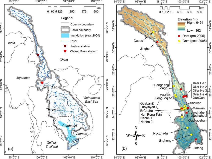
warming. The location of the gauging station (Chiang Saen) used for
In the remainder of the manuscript, we first describe the the calibration process is illustrated in Fig. 1a. This station
study area (Sect. 2) and then proceed by illustrating the com- provides a long and reliable daily time series, which has been
putational framework (Sect. 3), including the data on dams adopted by several studies on the Mekong basin (e.g., Lauri
and operating rules. In Sect. 4, we provide a detailed descrip- et al., 2012, 2014; Cochrane et al., 2014; Hoang et al., 2016).
tion of the results obtained for the aforementioned experi- To validate the model, we use monthly discharge values at
ments, whose implications are further discussed in Sect. 5. Jiuzhou station (see Fig. 1a), retrieved from He et al. (2009),
Wang et al. (2018), and Tang et al. (2019). For both stations,
we used data belonging to the period 1996–2005.
2 Study area The aforementioned orography and climate conditions are
not particularly suitable for agricultural activities, which are
The Mekong is a trans-boundary river that flows through indeed limited. The basin is mountainous, with mostly rocks
China, Myanmar, Thailand, and Laos before pouring into one and a shallow Quaternary alluvium (Carling, 2009; Gupta,
of the world’s largest deltas, located in Cambodia and Viet- 2009). Due to the impermeability of bedrock underneath iso-
nam. The catchment area of about 795 000 km2 can be di- lated valleys, only a very small fraction of water leaks into
vided into two parts, namely the upper Mekong, or Lancang, the ground through karst aquifer units (Lee et al., 2017). As
and the lower Mekong basins (Fig. 1a). The upper Mekong a result, subsurface water is mostly generated in the shallow
stretches in a north-to-south direction and drains an area of loam layer in the form of baseflow.
167 400 km2 . As shown in Fig. 1b, the region is characterized
by a complex orography, with high mountains and deep val-
leys (the elevation ranges from 362 to 6494 m). Because of 3 Materials and methods
these orographical conditions, the spatiotemporal variability
The first goal of our study is to investigate the role of water
of rainfall and temperature is remarkable. The average annual
reservoir storage and operations on the parameterization of
precipitation across the basin ranges from 752 to 1025 mm,
large-scale hydrological models. For this purpose, we adopt
70 % of which is concentrated in the monsoon season (May
the computational framework illustrated in Fig. 2, which con-
to November). The precipitation in the northwestern part of
sists of VIC’s rainfall–runoff and routing models and the ε-
the basin is sometimes lower than 250 mm yr−1 , making it
NSGA-II MOEA. In Sect. 3.1 we provide a detailed descrip-
dryer than the southeastern part, which receives an average of
tion of VIC, including the proposed variant for represent-
1600 mm yr−1 (Han et al., 2019). The average annual temper-
ing reservoir storage dynamics. The data and experimental
ature across the basin varies narrowly (from 12.3 to 14.3 ◦ C),
setup of the framework are outlined in Sect. 3.2 and 3.3. In
but the latitudinal temporal gradient is much larger – about
Sect. 3.4, we describe the climate change data used for our
2.2 ◦ C per 100 km (Wang et al., 2014). Climate changes are
second goal, that is, to demonstrate that different model pa-
expected to modify both rainfall and temperature patterns,
rameterizations caused by the absence (presence) of water
making the region warmer, wetter, and more susceptible to
reservoirs can affect the results of a climate change impact
extreme weather events (Tang et al., 2015).
assessment.
The favorable orography and abundant water availability
have attracted massive investments in the hydropower sector
(see the location of the dams in Fig. 1b), with consequent
impacts on the riverine ecosystems (Lauri et al., 2012; Dang
www.hydrol-earth-syst-sci.net/24/397/2020/ Hydrol. Earth Syst. Sci., 24, 397–416, 2020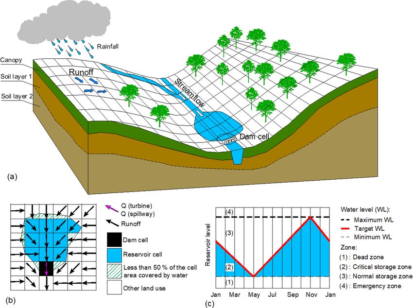
400                                                       T. D. Dang et al.: On the representation of water reservoir storage

Figure 1. Mekong river basin (a) and elevation map and location of the hydropower dams in the upper Mekong basin (b). The red squares
denote dams built before 2005 (and therefore included in our study), while the yellow circles indicate dams built after 2005.

3.1     Hydrological-water resources management model                ables are then used by the routing model (Lohmann et al.,
                                                                     1996, 1998), which simulates discharge throughout the river
3.1.1    Variable Infiltration Capacity model                        network using a linearized version of the Saint-Venant equa-
                                                                     tions. Specifically, the model first creates the impulse re-
VIC is a large-scale, semi-distributed land hydrological             sponse functions for each grid cell, and then simulates the
model maintained and developed by the University of                  flow convolution by aggregating the flow contribution from
Washington (http://www.hydro.washington.edu, last access:            all upstream cells at each time step lagged according the re-
22 January 2020). VIC consists of two core components,               sponse functions (ibid).
namely a rainfall–runoff and routing model (Fig. 2), which              Following the approach adopted in previous works on the
can be applied to multiple spatial scales and implemented            calibration of VIC (e.g., Dan et al., 2012; Park and Markus,
with different temporal resolutions – daily, in our case. The        2014; Xue et al., 2015), we focus our attention on six main
rainfall–runoff model simulates the water and energy fluxes          parameters that control the rainfall–runoff process (Table 1).
that govern the terrestrial hydrological cycle (Liang et al.,        These parameters are the thickness of the two soil layers (d1
1994). For these purposes, it takes as input climate forcings        and d2 ), the infiltration parameter (b), and three baseflow
(precipitation and temperature), land use and soil maps, leaf        parameters (Ds , Dmax , and Ws ). The parameter b character-
area index and albedo, and a digital elevation model (DEM).          izes the shape of the VIC curve, and therefore influences the
For each computational cell, the model uses one vegetation           available infiltration capacity and quantity of runoff gener-
layer and two (or three) soil layers: the upper soil layer con-      ated by each cell (for additional details, please refer to Ren-
trols evaporation, infiltration, and runoff, while the lower         Jun, 1992, and Todini, 1996). A higher value of b leads to a
layer controls the baseflow generation. These gridded vari-          lower infiltration rate and higher surface runoff. The three

Hydrol. Earth Syst. Sci., 24, 397–416, 2020                                         www.hydrol-earth-syst-sci.net/24/397/2020/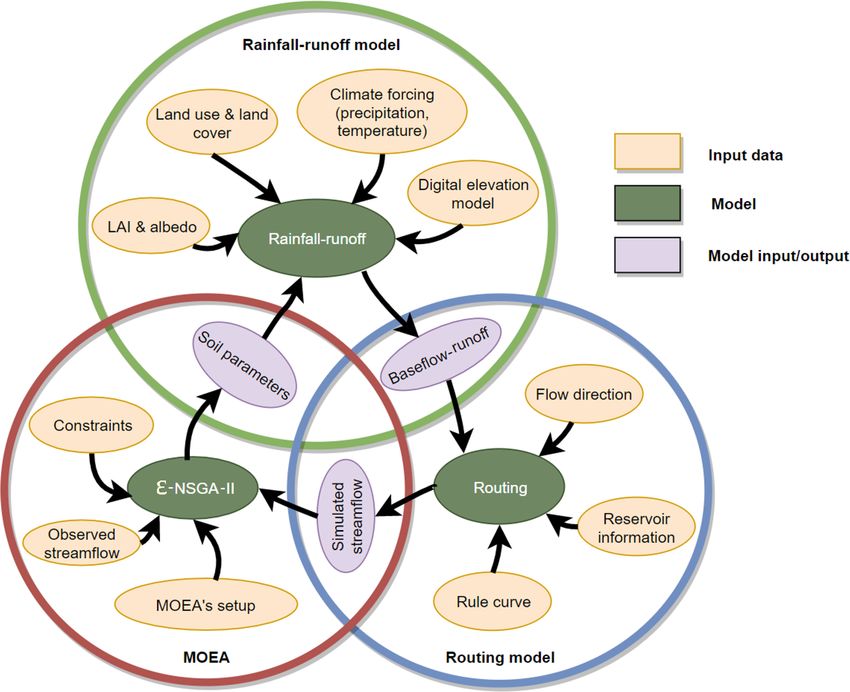
T. D. Dang et al.: On the representation of water reservoir storage                                                                401

Figure 2. Computational framework adopted in the first part of this study. The framework consists of VIC’s rainfall–runoff and routing
models and the MOEA ε-NSGA-II. The output of the rainfall–runoff model (i.e., gridded baseflow and runoff) is used by the routing model,
which simulates the streamflow at multiple locations within the upper Mekong basin. The simulated streamflow is then used to calculate
goodness-of-fit statistics, whose value is optimized with ε-NSGA-II by calibrating the parameters of the rainfall–runoff model. In other
words, these parameters and goodness-of-fit statistics represent the decision variables and objective functions used by ε-NSGA-II.

parameters Ds , Dmax , and Ws determine the shape of the              age in the dam cell, where we calculate the daily mass bal-
baseflow curve (Franchini and Pacciani, 1991), which re-              ance. From the dam cell, water is discharged using the rule
lates the soil moisture in the lower layer to the amount of           curves described in the following paragraph. Since the con-
baseflow. More specifically, Dmax is the maximum baseflow             struction of a dam is likely to create an impoundment with
that can occur in the lower layer, while Ds is the fraction of        surface area larger than the dam cell, we proceed by estimat-
Dmax associated with the transition from linear to nonlinear          ing the maximum reservoir extent, a factor used to determine
(rapidly increasing) baseflow generation. Ws is the fraction of       the so-called reservoir cells, namely cells that are at least
the maximum soil moisture (in the lower layer) where non-             half-covered by water (see Fig. 3b). Although these cells do
linear baseflow occurs. Hence, higher values of Ws increase           not contain the reservoir storage, they can affect the evapo-
the water content needed for rapidly increasing baseflow. The         ration processes, so their number and location must be deter-
thickness of the two soil layers affects several processes. In        mined accurately. The flow routing in these cells follows the
general, thicker layers delay the seasonal peak flow and in-          information provided in the flow direction map (described
crease the evaporation losses (since they increase the water          in Sect. 3.2.1). Further details about the implementation of
storage capacity).                                                    this variant of VIC’s routing model are given in Sect. S1 in
                                                                      the Supplement. We note that a more realistic way of repre-
3.1.2   Water reservoir storage and operations                        senting a reservoir within a hydrological model is to spread
                                                                      the reservoir storage over multiple upstream cells from the
To represent the storage dynamics of water reservoirs, we             dam location (Shin et al., 2019). However, a successful im-
modified VIC’s routing model (version 4.2) using the follow-          plementation of this method requires detailed bathymetry of
ing steps. First, we determine the location of all dams within        all reservoirs within the basin (information that may not al-
the basin and directly add them to the model using a dam              ways be available) and a 2-D model of the reservoir, so as
cell (Fig. 3a–b). To avoid allocating multiple dams within the        to accurately calculate the water fluxes between the different
same cell, we adopt a high spatial resolution of 0.0625◦ (ap-         reservoir cells.
proximately 6.9 km). Then, we aggregate the reservoir stor-

www.hydrol-earth-syst-sci.net/24/397/2020/                                             Hydrol. Earth Syst. Sci., 24, 397–416, 2020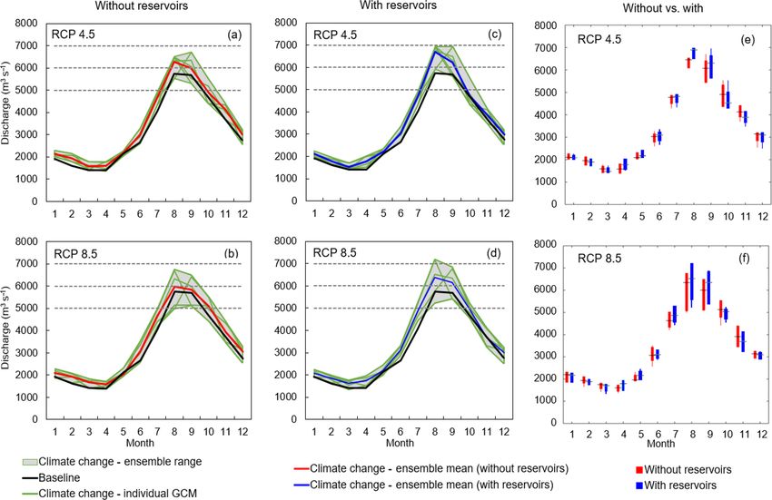
402                                                            T. D. Dang et al.: On the representation of water reservoir storage

Table 1. Main parameters controlling the rainfall–runoff process in VIC. The third column contains the range of each parameter value
considered during the calibration process. Note that these are the same ranges typically adopted for the implementation of VIC to large
basins (cf., Dan et al., 2012; Xue et al., 2015; Wi et al., 2017).

                Name     Unit        Feasible range     Description
                d1       m              [0.05, 0.25]    Thickness of the upper soil layer
                d2       m                 [0.3, 1.5]   Thickness of the lower soil layer
                b        –                   (0, 0.9]   Variable Infiltration Capacity curve parameter
                Dmax     mm d−1               (0, 30]   Maximum baseflow
                Ds       –                     (0, 1)   Fraction of Dmax where nonlinear baseflow begins
                Ws       –                     (0, 1)   Fraction of maximum soil moisture where nonlinear baseflow occurs

Figure 3. Graphical representation of VIC’s spatial domain (adapted from http://www.hydro.washington.edu, last access: 22 January 2020)
(a), including the selection of dam cell (black), reservoir cells (blue), and cells with other land use (white and white with green lines). The
black and pink arrows indicate the direction of the flow routing and discharge from the reservoir (b). Seasonal rule curve (c).

   As for the reservoir operations, we adopt an approach sim-             means determining the daily target water levels. For the case
ilar to that of Piman et al. (2012), which relies on rule curves          of hydropower production in the Mekong basin, such a rule
conceived to maximize the hydropower production – an as-                  should allow (1) drawdown of the reservoir storage during
sumption justified by the fact that all dams within the up-               the drier months (e.g., December to May) to maximize the
per Mekong are operated for hydropower supply (Räsänen                    production of electricity, (2) recharge of the depleted storage
et al., 2017). Determining the rule curve for a given reservoir           during the monsoon season, and (3) avoidance of the risks

Hydrol. Earth Syst. Sci., 24, 397–416, 2020                                               www.hydrol-earth-syst-sci.net/24/397/2020/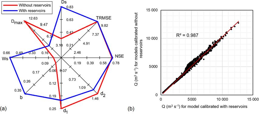
T. D. Dang et al.: On the representation of water reservoir storage 403
of spilling water at the end of the monsoon season (see the represented by the following equations:
illustration in Fig. 3c). Rule curves are tailored to each reser-
0 if St ≤ Sd (Zone 1)
voir within the basin by determining the time at which the
0 if Sd ≤ St ≤ Sts,tmodT and
minimum and maximum water levels are reached (May and
St + Qt − Et
November, in the Mekong; Piman et al., 2012), setting the
≤ Sts,tmodT (Zone 2, case 1)
value of the minimum and maximum water levels (the mini-
S ts,t modT − (S t + Qt − Et ) if Sd ≤ St ≤ Sts,tmodT and
mum and maximum elevation levels of each reservoir, in our St + Qt − Et
case), and finally connecting these points with a piecewise Rt = > Sts,tmodT (Zone 2, case 2) (2)
(St + Qt − Et ) − Sts,tmodT if Sts,tmodT ≤ St ≤ Scap and
linear function that gives us the daily target level for each
St + Qt − Et − Rmax
calendar day.
≤ Sts,tmodT (Zone 3, case 1)
As shown in Fig. 3c, there are three water levels that di-
Rmax if Sts,tmodT ≤ St ≤ Scap and
vide the storage into four zones. These levels are the dead
St + Qt − Et − Rmax
> Sts,tmodT (Zone 3, case 2)
water (or minimum elevation) level, the target water level,
and the full (or maximum elevation) level. If the water level
where Sd is the storage corresponding to the dead water level,
falls below the dead water level (Zone 1), the turbines are
and Sts,tmodT the target storage at time tmodT (in our study, we
not operated. If the level is between the dead water and tar-
use a period T of 365 d).
get level (Zone 2), the model first uses the information on the
incoming daily inflow to solve a mass balance equation, in 3.2 Data and preprocessing
which the discharge from the dam is kept at zero. The aim is
to understand whether the water level is expected to go be- 3.2.1 Climate forcings and other input variables
yond the target at the end of the day. If that is the case, the
model discharges through the turbines the amount of water Climate forcings are represented by precipitation and air tem-
needed to keep the level close to the target. Otherwise, the perature (maximum and minimum), which must be provided
turbines are not activated. In Zone 3 (between the target and at a daily time step. As far as precipitation is concerned, we
full level), the turbines are used at their maximum capacity, use the APHRODITE dataset (Asian Precipitation – Highly-
until the water reaches the target level. In Zone 4 (i.e., level Resolved Observational Data Integration Towards Evalua-
above the maximum elevation), both turbines and spillways tion), developed by the University of Tsukuba, Japan, using
are used. The key advantage of the rule curves adopted here rain-gauge data (Yatagai et al., 2012). APHRODITE is avail-
is that they do not require the calibration of any parameter. able with a spatial resolution of 0.25◦ and has been shown
Naturally, such an approach is less applicable when the infor- by Lauri et al. (2014) to be the most suitable precipitation
mation on the operating objectives is not available, or when dataset available for the Mekong basin. A similar observa-
dealing with multi-purpose water systems. tion applies to the CFSR (Climate Forecast System Reanaly-
Overall, our model implements the following mass bal- sis) maximum and minimum temperature dataset (Saha et al.,
ance equation at each simulation time step t (and for each 2014). These data are then interpolated to meet the spatial
reservoir): resolution of 0.0625◦ adopted in our implementation. More
specifically, we use the bilinear interpolation method, which
St+1 = St + Qt − Et − Rt , (1a) has found successful application in some recent studies (e.g.,
Hoang et al., 2016; Shin et al., 2019). We also bias correct the
0 ≤ St ≤ Scap , (1b) APHRODITE dataset (using a multiplying factor of 1.26), as
0 ≤ Rt ≤ min(St + Qt − Et , Rmax ), (1c) recommended by Lauri et al. (2014).
The monthly leaf area index and albedo are derived
where St is the reservoir storage at time t, Qt is the inflow from the Moderate Resolution Imaging Spectroradiometer
volume, Et is the evaporation loss, and Rt is the water re- (Terra MODIS) satellite images, which represent changes in
leased from the reservoir. Both storage St and discharge Rt canopy and snow coverage over time. (It is worth noting that
are constrained by the design specifications of each reservoir. snowmelt only marginally contributes to the streamflow of
Specifically, the storage cannot exceed the reservoir capacity the Mekong river; Räsänen et al., 2016.) Land use and land
Scap (Eq. 1b), while the discharge is bounded by the water cover data are obtained from the Global Land Cover Char-
availability and capacity of the turbines Rmax (Eq. 1c). The acterization (GLCC) dataset, developed by the United States
excess water, if any, is spilled: Geological Survey. We choose this product because it was
completed in 1993, close to the simulation period adopted in
our study (1995–2005). With such a choice, we make sure
Spillt = max(0, St + Qt − Rmax − Et − Scap ). (1d) that the influence of land use dynamics on the model pa-
rameterization is minimized. Soil data are extracted from the
Equation (1d) thus represents the release dynamics when Harmonized World Soil Database (HWSD), developed by the
the reservoir water level is in Zone 4. Zone 1, 2, and 3 are International Institute for Applied System Analysis and Food
www.hydrol-earth-syst-sci.net/24/397/2020/ Hydrol. Earth Syst. Sci., 24, 397–416, 2020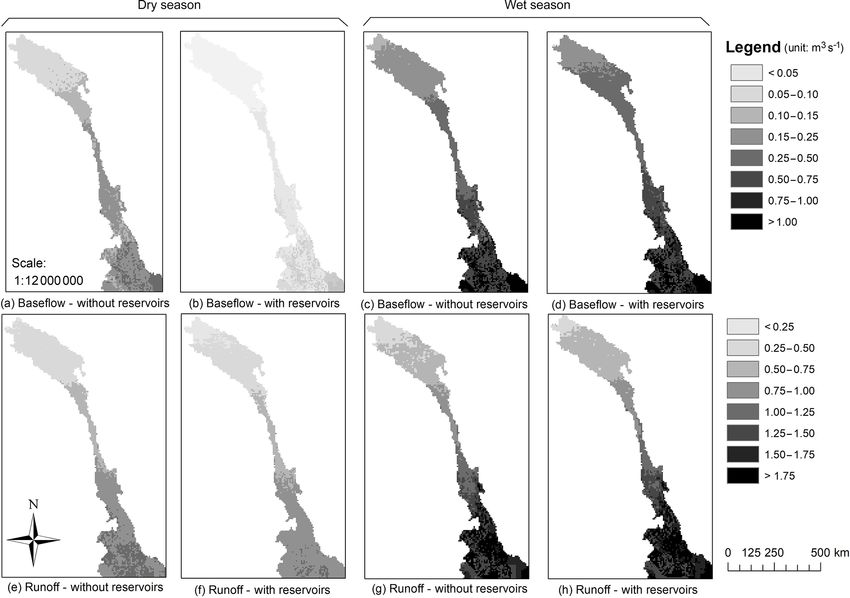
404 T. D. Dang et al.: On the representation of water reservoir storage
and Agriculture Organization and last updated in 2013. Both so we proceeded by analyzing remotely sensed data. More
land use and soil maps are generated with the majority re- specifically, we extracted surface water profiles from Land-
sampling technique, since their original spatial resolution is sat TM and ETM+ imagery. Landsat images are raster
30 arcsec (approximately 1 km). This technique assigns the grids with seven layers corresponding to seven bands (ex-
most common values found from the group of involved pixels cluding the panchromatic band). The normalized differ-
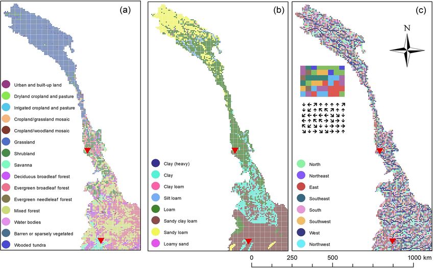
to the new cell. The resulting maps are illustrated in Fig. 4a– ence water index (NDWI) was calculated using the near-
b. The land use map shows that the upper reaches of the infrared (NIR, Band 4) and shortwave infrared (SWIR,
basin are characterized by the presence of grassland, while Band 5) bands: NDWI = (NIR − SWIR) / (NIR + SWIR).
the lower reaches – with complex terrain and large altitudi- Water bodies have NDWI values greater than 0.3 (McFeeters,
nal variations – present mixed coniferous forest ecoregions. 2013), so from the NDWI raster we can create a binary raster
Soil characteristics are also heterogeneous: in the central and in which 1 denotes a reservoir cell (and 0 a non-reservoir
northern part of the basin, soil is characterized by a shallow cell). This process yields an accurate estimation of the reser-
layer consisting of loam, sandy loam, and clay. At the bor- voir cells, since Landsat images have a spatial resolution of
der between China, Myanmar, and Laos (near Chiang Saen 30 m × 30 m.
station), soil characteristics are dominated by the presence of When calculating the daily mass balance for each reser-
sandy clay loam. voir, we consider three main processes, namely inflow, evap-
To estimate the flow directions, we use the Global oration, and release. Infiltration and seepage (via dam body,
30 arcsec Elevation (GTOPO30) DEM, which has been abutment, and foundation) are neglected. That is because of
adopted in several studies (e.g., Kite, 2001; Wu et al., 2012; two reasons. First, the upper Mekong basin is a mountainous
Li et al., 2013). First, we mask this DEM with the shape region, with mostly rocks and a shallow Quaternary alluvium
of the upper Mekong basin. Since GTOPO30 has a spatial (see Sect. 2), so infiltration losses are to some extent marginal
resolution of 30 arcsec, we then resample the DEM to the as compared to inflow, release, and evaporation. Second, the
resolution of our VIC model using the average resampling dams considered in our study are built with concrete (and
technique (Hoang et al., 2019). Finally, we manually correct with rocky abutments and foundations), so seepage is indeed
the flow direction map generated by ArcGIS by comparing limited.
it to a detailed river network provided by the Mekong River
Commission. Such correction is necessary, since errors are 3.3 Experimental setup
to some extent unavoidable when automatically generating a
flow direction map – because overland runoff and interflow To carry out the calibration exercise (with and without
directions depend on the relation between hillslope charac- reservoirs), we couple VIC with the ε-NSGA-II algorithm,
teristics and adopted spatial resolution. The resulting flow which has found successful application in many water re-
direction map is illustrated in Fig. 4c. sources problems – including model calibration (Reed et al.,
2013). In our case, the decision variables are represented
3.2.2 Dams and reservoir information by the six parameters controlling the rainfall–runoff process
in VIC (Sect. 3.1.1), and whose range of variability is re-
Our model requires detailed information on the reservoirs, ported in Table 1. As for the objective functions, we consider
namely location, storage capacity, dam height, dead storage, two goodness-of-fit statistics dependent upon the simulated
turbine design discharge, and maximum and minimum el- streamflow, namely the Nash–Sutcliffe efficiency (NSE) and
evation levels. Such information (summarized in Table 2) transformed root mean square error (TRMSE), which assess
was retrieved by cross-checking the databases provided by the model performance on high and low flows, respectively
the Mekong River Commission, the International Commis- (Dawson et al., 2007). The NSE is defined as follows:
Pn
sion On Large Dams, and the Global Reservoir and Dam (Qt − Qto )2
Database. Since data on reservoir bathymetry are not avail- NSE = 1 − Pnt=1 s , (3)
t 2
t=1 (Qo − Qo )
able, we modeled the storage–depth relationship with Liebe’s
method, which assumes that the reservoir is shaped like a top- where n is the number of time steps, Qts is the simulated
down pyramid cut diagonally in half (Liebe et al., 2005). In streamflow (at time t), Qto is the observed streamflow (at
other words, the relation between reservoir volume (V ) and Chiang Saen station), and Qo is the mean of the observed
depth (or level, h) is equal to V = ah3 , where a is a shape streamflow. The TRMSE is defined as follows:
factor equal to Vcap /h3max (Vcap is the live storage capacity v
u n
and hmax the maximum water depth). This method has been u1 X
TRMSE = t (zs,t − zo,t )2 , (4)
adopted for regional and global studies (see Ng et al., 2017; n t=1
Shin et al., 2019).
As for the maximum reservoir extent (needed to deter- where zs,t and zo,t represent the value of the simulated and
mine the reservoir cells), the existing databases do not pro- observed streamflow (at time t) transformed by the expres-
λ −1
vide detailed information, such as the reservoir polygon, sion z = (1+Q)
λ , (λ = 0.3). In other words, λ scales down
Hydrol. Earth Syst. Sci., 24, 397–416, 2020 www.hydrol-earth-syst-sci.net/24/397/2020/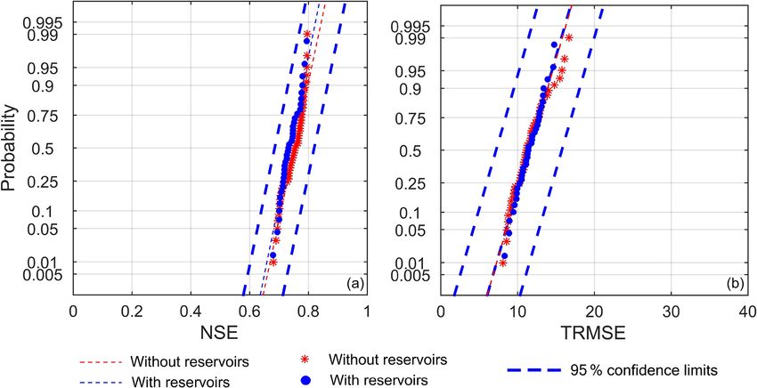
T. D. Dang et al.: On the representation of water reservoir storage                                                                405

Figure 4. Land use map derived from the Global Land Cover Characterization dataset (a); soil map (for the top layer) retrieved from the
Harmonized World Soil Database (b); flow direction map (c). The red triangles denote the position of the Chiang Saen and Jiuzhou gauging
stations.

the values of the streamflow, and TRMSE thus emphasizes               to be parallelized. For each of the 20 seeds, we used four
the errors on the low flows. In this specific modeling prob-          cores, taking approximately 200 h per core (wall-clock time).
lem, capturing both high and low flows is particularly impor-            Since 6 (out of 11) dams became operational during the
tant, since the riverine ecosystems are sensitive to both dry         study period (see Table 2), the VIC simulation with reser-
and wet conditions (Hoang et al., 2016).                              voirs is implemented in such a way to activate the reservoirs
   Both objective functions are calculated for the period             at the right time. In this specific implementation, we do not
1996–2005 – after a 1-year spin-up period, 1995 – and scaled          use filling strategies different from the rule curves described
between 0 and 1, so we set only one value of ε (equal to              in Sect. 3.2.2, because all six dams reach a steady-state oper-
0.001). The other ε-NSGA-II parameters to set up are the size         ation within a few months (data not shown).
of the initial population and number of function evaluations,
which are equal to 10 and 250 – a setting that strikes a rea-         3.4   Climate change data
sonable balance between the computational requirements of
the calibration exercise and the quality of the solutions. Each       For our second experiment, we used the CMIP5 climate
calibration exercise (with and without reservoirs) is solved          projections to derive climate change scenarios for the pe-
with 20 different random seeds, so as to characterize the vari-       riod 2050–2060. Since the data provided by the Coordinated
ability in the ε-NSGA-II stochastic search process. The fi-           Regional Climate Downscaling Experiment only cover one
nal set of Pareto-efficient solutions (i.e., alternative param-       GCM for our study site (Giorgi and Gutowski Jr., 2015), we
eterizations of VIC) thus corresponds to the set of Pareto-           followed the approach taken by previous studies (e.g., Hoang
efficient solutions identified across all 20 seeds. All experi-       et al., 2016, 2019) and proceeded by using GCM projec-
ments are carried out on an Intel (R) Xeon (R) W-2175 CPU             tions as a basis for our scenarios. As far as the GCMs are
2.50 GHz with 128 GB RAM running Linux Ubuntu 16.04                   concerned, we used ACCESS1-0, CCSM4, CSIRO Mk3.6,
(Xenial Xerus), using a Python implementation of various              HadGEM2-ES, and MPI-ESM-LR, whose reliability for this
MOEAs (Platypus) that allows the optimization experiments             region has been evaluated in a few previous studies (Sill-
                                                                      mann et al., 2013; Huang et al., 2014; Ul Hasson et al.,
                                                                      2016; Hoang et al., 2016). The main characteristics of the

www.hydrol-earth-syst-sci.net/24/397/2020/                                             Hydrol. Earth Syst. Sci., 24, 397–416, 2020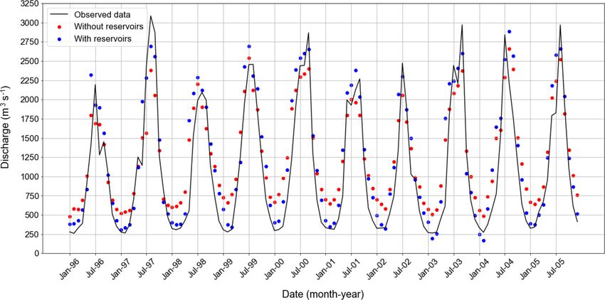
406                                                         T. D. Dang et al.: On the representation of water reservoir storage

Table 2. Design specifications of the dams implemented in our VIC model (simulation period 1995–2005). The column marked “Year”
denotes the year in which each reservoir became operational.

             No.          Name         Year    Long.      Lat.     Height        Storage   Design discharge   Installed capacity
                                                (◦ E)    (◦ N)       (m)         (Mm3 )           (m3 s−1 )               (MW)
             1            Xi’er He 4   1971   100.066   20.000            20          14               283                   50
             2            Xi’er He 1   1989   100.202   30.000            30      1,501                  60                 105
             3            Xi’er He 2   1987   100.131   25.562         37.25         0.2               168                   50
             4            Xi’er He 3   1988   100.108   20.700         20.70       0.09                304                   50
             5            Manwan       1992   100.446   24.625           136        257              1,700                1,670
             6            Longdi       1997    99.724   26.221            95      13.30              12.34                   10
             7            Laoyinyan    1997    99.818   24.469          4.31      10.92                 9.3                  16
             8            XunCun       1999    99.993   25.422            67      73.74                146                   78
             9            Jinfeng      1998   101.225   21.592            45      19.48                  45                  16
             10           Dachaoshan   2003   100.370   24.025           115        367              2,109                 1350
             11           Jinhe        2004    97.333   34.000            34       4.27                222                   60

GCMs are summarized in Table 3. As for the RCPs, we chose                  river discharges (Lauri et al., 2012, 2014). More recently,
RCPs 4.5 and 8.5. The former is a medium-to-low scenario                   some studies have focussed on hydrological extremes, such
that assumes a stabilization of radiative forcing to 4.5 W m−2             as high (Q5 ) and low flows (Q95 ) (Hoang et al., 2016). Since
by 2100, while the latter is a high emission scenario based                our goal is to demonstrate that different model parameteriza-
on an increase of the radiative forcing to 8.5 W m−2 by 2100.              tions caused by the absence (or presence) of water reservoirs
These two RCPs provide a broad range of climate variability                can largely impact the results of climate change assessments
for the region – and thus exclude RCP 2.6, which is charac-                – and not to push forward the boundaries of climate change
terized by the lowest radiative forcings.                                  impact assessments – we chose a simple and established cri-
   To prepare the precipitation and temperature data used by               terion, namely the annual and monthly river discharges at
VIC, we then re-gridded and bias corrected the GCMs out-                   Chiang Saen and Jiuzhou stations.
puts. The first step is necessary to overcome the limited spa-
tial resolution of the GCMs (our VIC implementation uses
a resolution of 0.0625◦ × 0.0625◦ ) and is carried out using               4     Results
the bilinear interpolation method. The bias correction is per-
formed with the delta method (Diaz-Nieto and Wilby, 2005;                  To discuss the impact of water reservoirs on the parameter-
Choi et al., 2009), which has already been applied to our                  ization of hydrological models, we first compare the results
study site (Lauri et al., 2012). With this method, we calculate            of the calibration exercise carried out with and without reser-
correcting factors for precipitation and temperature using the             voirs and then proceed by comparing the performance of two
following expressions:                                                     selected parameterizations on the climate change impact as-
                                                                           sessment.
         P series,i
1PRE =                ,                                          (5)       4.1     Model parameterization
          P ref,i
           T series,i − T ref,i                                            The optimization-based parameterization exercise yielded a
1TEMP =                         ,                                (6)       total of 118 and 109 parameterizations (or Pareto-efficient
                  σref,i
                                                                           solutions) for the VIC implementations with and without
where P series,i and T series,i are the (11-year) average precip-          reservoirs, respectively. To prove our hypothesis that the cal-
itation and temperature for month i produced by the GCM                    ibration process may somehow compensate for a deficiency
in our control period (1995–2005), P ref,i and T ref,i are the             in the model structure – the absence of reservoirs, in our
(11-year) average observed precipitation and temperature for               case – we begin by analyzing the values of the goodness-
month i in the period 1995–2005, and σref,i is the stan-                   of-fit statistics, namely NSE and TRMSE. Figure 5 reports
dard deviation of the monthly average temperature during                   the probability plots of NSE and TRMSE values obtained
the same period for month i. These factors were then used                  for the two model setups: results show that the calibration
to correct the future climate projections for each time series             exercise yields a reasonable modeling accuracy, with NSE
(using the same factor for all daily data in a given month).               and TRMSE varying in the ranges 0.68–0.79 and 8.10–
   The impact of climate change on hydrological processes is               16.69. More interestingly, these results show that the NSE
often assessed by studying changes in the flow regime, and,                and TRMSE values of both model setups belong to the same
in particular, changes in the monthly, seasonal, and annual                range of variability and follow an almost identical distribu-

Hydrol. Earth Syst. Sci., 24, 397–416, 2020                                                 www.hydrol-earth-syst-sci.net/24/397/2020/
T. D. Dang et al.: On the representation of water reservoir storage 407
Table 3. CMIP5 GCMs used for the climate change impact assessment.
GCM Spatial resolution Control baseline Developer
(long × lat)
ACCESS1-0 1.875◦ × 1.25◦ 1850–2006 Commonwealth Scientific and Industrial Research
Organization, Australia
CCSM4 1.25◦ × 0.94◦ 1850–2005 National Center for Atmospheric Research, USA
CSIRO Mk3.6 1.875◦ × 1.875◦ 1850–2005 Commonwealth Scientific and Industrial Research Organization
and the Queensland Climate Change Centre of Excellence,
Australia
HadGEM2 ES 1.875◦ × 1.24◦ 1861–2010 Met Office, UK
MPI-ESM-LR 1.875◦ × 1.875◦ 1850–2005 Max Planck Institute for Meteorology, Germany
tion. In addition, all NSE and TRMSE values of the mod- lower layer. Finally, we can note that d1 (the thickness of
els without reservoirs fall within the 95 % confidence lim- the first layer) in the models without reservoirs tends to be
its calculated using the NSE and TRMSE values attained by larger, indicating that these model instances increase the wa-
the models with reservoirs. To corroborate this finding, we ter storage capacity of the top layer. The only parameter that
carried out a Kolmogorov–Smirnov two-sample test to re- does not appear to depend on the absence (or presence) of
ject the null hypothesis that the values of NSE (and TRMSE) water reservoirs is d2 , the thickness of the second soil layer.
produced by the two model setups come from the same dis- This result is corroborated by a global sensitivity analysis,
tribution. For both goodness-of-fit statistics, the hypothesis which shows that d2 is indeed the parameter with the least
cannot be rejected (with a 5 % significance level). Overall, influence on the model output (Fig. S2 in the Supplement).
this confirms that the accuracy of the models is not affected Overall, it appears that the calibration process compensates
by the presence (absence) of the reservoirs. for the absence of water reservoirs by determining values of
How does the parameterization compensate for the ab- the soil parameters that can somehow ‘mimic’ the alterations
sence of water reservoirs? To answer this question, we vi- caused by water reservoirs, namely an increase in the evap-
sualize both goodness-of-fit statistics (NSE and TRMSE) oration and delay in the peak flows – obtained by increasing
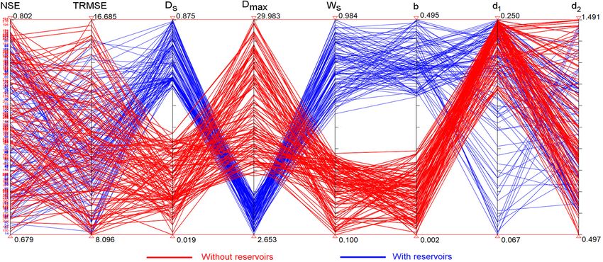
and model parameters (Ds , Dmax , Ws , b, d1 and d2 ) in a infiltration, baseflow, and soil water storage capacity.
parallel-coordinate plot (Fig. 6). These eight variables are To further understand the unintended consequences of the
shown in eight parallel axes, so each line connecting the absence of water reservoirs, we select two model parameter-
axes represents a parameterization (i.e., a solution of the opti- izations (with and without reservoirs) characterized by the
mization problem) along with the corresponding value of the same performance over the period 1996–2005. The values
goodness-of-fit statistics (i.e., the objectives). Blue and red of NSE, TRMSE, and model parameters are illustrated in
lines denote solutions obtained with and without reservoirs, Fig. 7a, while the simulated daily discharges produced by
respectively. First of all, one can notice that while NSE and both models are compared in the scatter plot of Fig. 7b. In
TRMSE spread over the same ranges (results discussed in Fig. 8, we contrast the average values of simulated base-
the previous paragraph), the presence or absence of reser- flow and runoff during the dry (December–April) and wet
voirs consistently yields different parameterizations. Let’s (May–November) seasons of the period 1996–2005. Unsur-
analyze them. The value of b – characterizing the shape of the prisingly, results show that during the dry season the model
VIC curve – belongs to two distinct ranges (0.319–0.495 and without reservoirs generates more baseflow and runoff than
0.002–0.195) for the model implementation with and with- the model with reservoirs (left four panels of Fig. 8): dur-
out reservoirs, respectively, indicating that the model with- ing the dry months, hydropower reservoirs release part of the
out reservoirs has higher infiltration and lower surface runoff water stored during the monsoon (recall the rule curves de-
than the model with reservoirs (recall that a higher value of scribed in Sect. 3.1.2) – a process simulated by the model
b leads to a lower infiltration rate and higher surface runoff; without reservoirs by increasing both baseflow and runoff –
Sect. 3.1.1). A similar observation applies to the parameters and, therefore, the discharge at the catchment outlet. During
Ds , Dmax , and Ws , which determine the shape of the baseflow the wet season, we find an opposite trend: in these months,
curve. In this case, the model without reservoirs has higher hydropower reservoirs tend to store part of the water (thus
values of Dmax (i.e., maximum baseflow) and lower values reducing the discharge at the catchment outlet), so the model
of Ds and Ws (i.e., fraction of Dmax where rapidly increasing without reservoirs slightly decreases the discharge by reduc-
baseflow begins, and fraction of the maximum soil moisture ing baseflow and runoff (right four panels of Fig. 8). We also
in the lower layer where rapidly increasing baseflow occurs), note that the difference between the two models is clearer
suggesting that the absence of reservoirs leads to model pa- during the dry season, when a larger amount of the water
rameterizations that favor the generation of baseflow in the volumes is controlled by the hydropower reservoirs.
www.hydrol-earth-syst-sci.net/24/397/2020/ Hydrol. Earth Syst. Sci., 24, 397–416, 2020408 T. D. Dang et al.: On the representation of water reservoir storage
Figure 5. Probability plots for the NSE (a) and TRMSE (b) obtained in the model calibration process. The blue circles and red stars
specify the results obtained by the models with and without reservoirs, respectively. The dashed blue and red lines represent the theoretical
distributions. In both plots, we also report the 95 % confidence limits for the models calibrated with reservoirs.
Figure 6. Parallel coordinate plot illustrating the values of the goodness-of-fit statistics (NSE and TRMSE) and model parameters (Ds ,
Dmax , Ws , b, d1 and d2 ) obtained through the optimization-based parameterization exercise. Each line connecting the axes represents a
parameterization, along with the corresponding model performance. Blue and red lines denote parameterizations obtained with and without
reservoirs.
The effect of such flawed representation of baseflow and applications of the models, such as a climate change impact
runoff is further demonstrated by validating the simulated assessment.
discharge at Jiuzhou station. Figure 9 shows a macroscopic
difference between the models calibrated with and without 4.2 Climate change impact assessment
reservoirs. In particular we note that the model calibrated
without reservoirs largely overestimates the dry season flow
To begin the climate change impact assessment, we compare
and slightly underestimates the wet season one; a result con-
the data produced by the GCMs over the reference and fu-
firmed by the values of NSE (equal to 0.82 and 0.79 for
ture period (1996–2005 and 2050–2060). In general, the to-
the model with and without reservoirs) and TRMSE (equal
tal annual precipitation in the Lancang basin is projected to
to 21.48 and 28.95). One may also suspect that these unin-
increase under almost all climate change scenarios – only the
tended consequences could further propagate in downstream
CSIRO MK3-RCP 8.5 scenario projects a −3.12 % decrease
in the total annual precipitation. Yet, we observe a large spa-
Hydrol. Earth Syst. Sci., 24, 397–416, 2020 www.hydrol-earth-syst-sci.net/24/397/2020/T. D. Dang et al.: On the representation of water reservoir storage 409 Figure 7. Radar chart illustrating the values of the Nash–Sutcliffe efficiency (NSE), transformed root mean square error (TRMSE), and model parameters (Ds , Dmax , Ws , b, d1 and d2 ) of the two selected models (a); scatter plot comparing the daily discharges at Chiang Saen station simulated by the two models over the period 1996–2005 (b). Figure 8. Average values of simulated baseflow (a, b, c, d) and runoff (e, f, g, h) simulated by the selected models (with and without reservoirs) during the dry (December–April) and wet (May–November) seasons of the period 1996–2005. www.hydrol-earth-syst-sci.net/24/397/2020/ Hydrol. Earth Syst. Sci., 24, 397–416, 2020
410                                                         T. D. Dang et al.: On the representation of water reservoir storage

tial variability in the total annual rainfall within each scenario   ceive larger inflows, part of which is directly spilled into the
(see Fig. S3). For example, in ACCESS-RCP 4.5, rainfall              downstream reaches (data not shown). This is an unprece-
changes vary between −2 % in the central part of the basin           dented situation for the model without reservoirs, which can-
to more than +10 % in the southern part. All scenarios (but          not simulate an increase in the use of the spillways. In fact,
for CSIRO MK3-RCP 8.5) tend to share a similar spatial pat-          this model tends to reproduce the dynamics learned during
tern, in which the lower part of the basin exhibits an increase      the calibration process, that is, storing part of the water (in
in the projected precipitation. As for the temperature, we ob-       the lower soil layer) during the monsoon season and slowly
serve an increase in both minimum and maximum tempera-               discharging it in the following months.
ture across all scenarios (see Fig. S4), with higher warming            Naturally, the difference between the monthly discharges
for the RCP 8.5. Also in this case, we can note some vari-           predicted by the two models becomes even more apparent
ability across the GCMs as well as the spatial domain. As            when we consider Jiuzhou station, which was not used in
discussed in Hoang et al. (2016), these precipitation and tem-       the calibration process. As depicted in Fig. 11, the model
perature scenarios represent an improvement with respect to          without reservoirs consistently yields higher discharges in
the CMIP3 ones, which show a broader variability. However,           the pre-monsoon season and lower discharges in the mon-
there still are some non-negligible differences across the sce-      soon season. Note that, in some months, the difference be-
narios that are likely to cause different projections of the an-     tween the average monthly discharges produced by the two
nual and monthly river discharges.                                   models causes an uncertainty larger than the one surrounding
   The expected climate change impacts on the annual river           the downscaled climate projections. For instance, the average
discharge at Chiang Saen are synthesized in Table 4, where           monthly discharge in March (under both RCPs) predicted by
we report the relative changes in discharge with respect to the      two models is about 500 and 750 m3 s−1 , that is, a 50 % dif-
period 1996–2005. Interestingly, it appears that the projec-         ference.
tions are robust with respect to the representation of the wa-
ter reservoirs. Indeed, the model with and without reservoirs
yield comparable ensemble means and ranges for the two               5   Discussion and conclusions
RCPs. Specifically, we find that the annual discharge is pre-
dicted to increase in the vast majority of the scenarios, in re-     This work contributes to the existing literature on large-
sponse to the increase in precipitation described above. Such        scale hydrological modeling by studying the effect of wa-
similarity between the projections is arguably attributable to       ter reservoir storage and operations on the parameterization
the calibration process, which generates models producing            of process-based models. To this purpose, we developed a
similar aggregate performance measures at Chiang Saen sta-           computational framework consisting of VIC and the multi-
tion.                                                                objective evolutionary algorithm ε-NSGA-II, which we used
   What is perhaps more interesting is a comparison between          to calibrate the model parameters through a simulation–
the monthly discharges at Chiang Saen predicted by the mod-          optimization process. Our framework also includes a novel
els with and without reservoirs. While both models produce           variant of VIC that simulates both storage dynamics and op-
similar ensemble ranges (see Fig. 10a–d), a closer analysis of       erations of water reservoirs. Using the Lancang river basin as
the data reveals a non-negligible difference in the minimum,         a case study, we calibrated two implementations of VIC, with
maximum, and average monthly discharges (across the GCM              and without reservoirs. In line with previous studies (e.g.,
scenarios) produced by the two models (Fig. 10e–f). In par-          de Paiva et al., 2013; Abbaspour et al., 2015), we found that
ticular, the model with reservoirs predicts higher discharges        the model without reservoirs attains a reasonable modeling
in the July–September period and lower discharges in Oc-             accuracy. In fact, we found that the calibration process of
tober and November. Note that such difference is consistent          both model implementations yields de facto the same values
across both RCPs. Since both models share the same rain-             of the goodness-of-fit statistics (NSE and TRMSE), suggest-
fall and temperature scenarios, the only cause for this stark        ing that the model parameterization helps compensates for a
difference must lie in the unintended consequences of the pa-        structural error, namely the absence of the water reservoirs.
rameterization process. As explained in Sect. 4.1, the model         More specifically, this effect is achieved by determining the
without reservoirs shows two “artifacts” that help compen-           values of six soil parameters (Ds , Dmax , Ws , b, d1 and d2 )
sate for the absence of the hydropower reservoirs: first, it in-     that let this model implementation emulate the presence of
creases both baseflow and runoff during the dry season (to           water reservoirs.
account for the water discharged to sustain hydropower pro-             The first implication of a flawed parameter estimation
duction in the dry months); second, it decreases baseflow and        stands in a poor representation of key hydrological pro-
runoff (to account for part of the water stored by the dams          cesses, such as surface runoff, infiltration, and baseflow. In
during the wet months). The latter artifact is responsible for       our case, we found that, during the dry months, the models
the macroscopic change in the hydrograph described above.            calibrated without water reservoirs generate a higher amount
In the wetter conditions depicted by the GCM and RCP sce-            of baseflow and runoff than the models with reservoirs.
narios, the hydropower reservoirs of the Lancang basin re-           This is an artifact needed to reproduce the higher discharges

Hydrol. Earth Syst. Sci., 24, 397–416, 2020                                         www.hydrol-earth-syst-sci.net/24/397/2020/
You can also read