State-space optimal feedback control of optogenetically driven neural activity
←
→
Page content transcription
If your browser does not render page correctly, please read the page content below
Journal of Neural Engineering

PAPER

State-space optimal feedback control of optogenetically driven neural
activity
To cite this article: M F Bolus et al 2021 J. Neural Eng. 18 036006

View the article online for updates and enhancements.

                              This content was downloaded from IP address 143.215.137.43 on 26/05/2021 at 13:34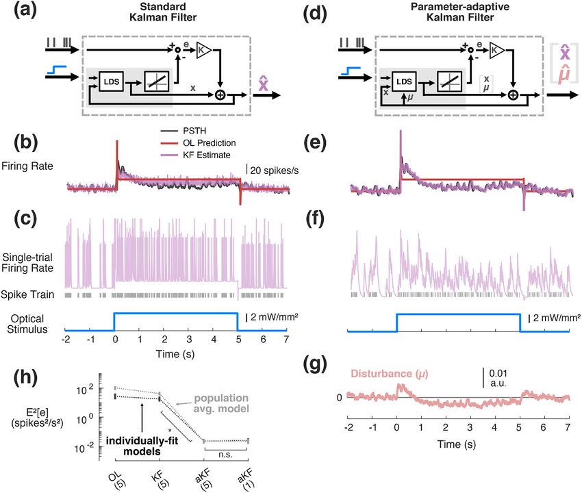
J. Neural Eng. 18 (2021) 036006 https://doi.org/10.1088/1741-2552/abb89c
Journal of Neural Engineering
PAPER
State-space optimal feedback control of optogenetically driven
RECEIVED
25 June 2020
REVISED
neural activity
26 August 2020
M F Bolus1, A A Willats1, C J Rozell2 and G B Stanley1
ACCEPTED FOR PUBLICATION
15 September 2020 1
Wallace H. Coulter Department of Biomedical Engineering, Georgia Institute of Technology and Emory University, Atlanta, GA 30332,
PUBLISHED United States of America
31 March 2021 2
School of Electrical and Computer Engineering, Georgia Institute of Technology, Atlanta, Georgia 30332, United States of America
E-mail: garrett.stanley@bme.gatech.edu
Keywords: closed-loop, control, estimation, optogenetics, state space, thalamus, firing rate, in vivo
Abstract
Objective. The rapid acceleration of tools for recording neuronal populations and targeted
optogenetic manipulation has enabled real-time, feedback control of neuronal circuits in the brain.
Continuously-graded control of measured neuronal activity poses a wide range of technical
challenges, which we address through a combination of optogenetic stimulation and a state-space
optimal control framework implemented in the thalamocortical circuit of the awake mouse.
Approach. Closed-loop optogenetic control of neurons was performed in real-time via stimulation
of channelrhodopsin-2 expressed in the somatosensory thalamus of the head-fixed mouse. A
state-space linear dynamical system model structure was used to approximate the light-to-spiking
input-output relationship in both single-neuron as well as multi-neuron scenarios when recording
from multielectrode arrays. These models were utilized to design state feedback controller gains by
way of linear quadratic optimal control and were also used online for estimation of state feedback,
where a parameter-adaptive Kalman filter provided robustness to model-mismatch.
Main results. This model-based control scheme proved effective for feedback control of
single-neuron firing rate in the thalamus of awake animals. Notably, the graded optical actuation
utilized here did not synchronize simultaneously recorded neurons, but heterogeneity across the
neuronal population resulted in a varied response to stimulation. Simulated multi-output feedback
control provided better control of a heterogeneous population and demonstrated how the
approach generalizes beyond single-neuron applications. Significance. To our knowledge, this work
represents the first experimental application of state space model-based feedback control for
optogenetic stimulation. In combination with linear quadratic optimal control, the approaches laid
out and tested here should generalize to future problems involving the control of highly complex
neural circuits. More generally, feedback control of neuronal circuits opens the door to adaptively
interacting with the dynamics underlying sensory, motor, and cognitive signaling, enabling a
deeper understanding of circuit function and ultimately the control of function in the face of
injury or disease.
1. Introduction to a wide range of discoveries of the circuit mechan-
isms underlying sensory, motor, and cognitive pro-
Over the last two decades, there has been a rapid cesses [4]. The integration of recording and opto-
expansion of tools and technologies for recording the genetic stimulation techniques, however, has received
large-scale activity within and across brain structures comparatively little attention until recently ([5–13];
at single neuron resolution [1, 2]. In parallel, the for review [14]), and in most cases these closed-
development of optogenetics provided the ability to loop systems utilize event-triggered or on-off con-
optically excite or inhibit neural activity in a cell-type trol rather than continuous feedback. While feed-
specific manner [3]. Together, these advances in the back control is the engineering cornerstone for the
ability to ‘read’ or ‘write’ the neural code have led function of a wide range of complex technologies
© 2021 IOP Publishing LtdJ. Neural Eng. 18 (2021) 036006 M F Bolus et al
ranging from communication to flight, applying this was carried out via optical activation of the excit-
perspective in the nervous system remains more the- atory opsin channelrhodopsin-2 (ChR2) expressed
oretical [15–19] than experimental. In this study, in the somatosensory thalamus of the awake, head-
we establish a general framework for continuously fixed mouse. A feedback controller updated light
modulated closed-loop optogenetic control of neur- intensity in real-time based on simultaneous elec-
onal circuits, where optical actuation is determined trophysiological measurements of the thalamic neur-
in real-time by comparing measured neuronal spik- ons being manipulated. A linear dynamical system
ing to target activity. This work opens up possibilities model structure was used to approximate the light-
for investigation of poorly understood mechanisms to-spiking input-output relationship in both single-
of the underlying circuitry and for adaptively inter- neuron as well as multi-neuron scenarios in cases
acting with the circuit dynamics within and across where multiple neurons were measured simultan-
brain regions that constantly change in response to eously using multielectrode arrays. These linear state-
the internal and external environments. space models were used in combination with linear
Electrical stimulation has been the gold stand- quadratic optimal control to design feedback control-
ard for manipulating the activity of neurons at fast ler gains for the purpose of regulating thalamic firing
time-scales, and remains the basis for clinical inter- around a desired target rate. The models were also
ventions like deep brain stimulation [20]. However, used online for estimation of state feedback, using
this approach suffers from lack of specificity while a parameter-adaptive Kalman filter for robustness to
also typically precluding simultaneous measurement model-mismatch. The resulting controller-estimator
of the activity of the neurons being stimulated. While feedback loop was deployed experimentally by way of
not yet clinically viable, optogenetics offers an altern- a custom-written program running in real-time. This
ative approach that enables cell-type specificity, bi- control scheme provided effective optogenetic con-
directional actuation, the ability to simultaneously trol of firing rate in the awake brain, owing to the
stimulate and obtain electrophysiological recordings, robustness to model accuracy granted by a parameter-
and a potentially lesser degree of unnatural synchron- adaptive Kalman filter that estimated a stochastically-
ization of the local population [21]. This presents an varying process disturbance. Feedback control using
attractive toolbox for the development of continu- this estimator resulted in very good firing rate track-
ous, feedback control strategies where stimulation is ing experimentally for the single neurons whose activ-
continuously modulated based on real-time measure- ity was used for feedback. By comparison, control was
ments of the local neuronal activity. There has been a not as effective for other simultaneously-measured
range of studies where previously-determined stim- neurons not used for feedback. To investigate the gen-
ulation is triggered based on recorded activity in a eralizability and efficacy of these methods for future
reactive closed-loop fashion [8–11]. In addition to multi-output control scenarios, we demonstrate their
event-triggered control, a recent study has also used application to multi-neuron feedback control of a
on-off closed-loop control to gate photostimulation population in simulation.
when recorded neuronal activity was below target
levels [13]. Although these approaches to stimula- 2. Methods
tion have proven effective for their uses, they are fun-
damentally different from the continuously-graded 2.1. Animal preparation
feedback control we describe here, where stimula- All procedures were approved by the Institutional
tion is updated on a moment-by-moment basis as Animal Care and Use Committee at the Georgia
a function of the current and past measured neural Institute of Technology and were in agreement with
activity. In previous studies, we have developed and guidelines established by the NIH. Experiments were
demonstrated strategies for closed-loop optogenetic carried out using either C57BL/6 J mice that were
control of spiking activity of neurons in a cultured virally transfected to express channelrhodopsin-2
network and single neurons in vivo in the anesthetized (ChR2) or by single-generation crosses of an Ai32
brain [5, 7]. While laying the conceptual groundwork, mouse (Jax) with an NR133 cre-recombinase driver
these approaches do not scale well to neuronal pop- line (Jax) which grants better specificity of ChR2
ulations and do not take advantage of more modern expression in ventral posteromedial/posterolateral
approaches in control theory. Additionally, these pre- thalamus [22]. In the case of viral transfection, ChR2
vious studies had not yet applied optogenetic control expression was targeted to excitatory neurons in the
in the context of wakefulness. thalamus via stereotactic injection relative to bregma
In this study we bridge the gap between opto- (approximately 2 × 2 × 3.25 mm caudal × lateral
genetics and established paradigms of more modern × depth) using 0.5 µL of virus (rAAV5/CamKIIa-
control theory by utilizing state-space models to cap- hChR2(H134R)-mCherry-WPRE-pA; UNC Vector
ture single- and multi-neuron responses to optogen- Core, Chapel Hill, NC) at a rate of 1 nL/s.
etic stimulation and employing optimal control to At least three weeks prior to recordings, a custom-
design the control loop for driving desired neuronal made metal plate was affixed to the skull for head
activity. Specifically, precise manipulation of neurons fixation, and a recording chamber was made using
2J. Neural Eng. 18 (2021) 036006 M F Bolus et al
dental cement while the animals were maintained controller gains to a state-space controller object, and
under 1%–2% isoflurane anesthesia [23]. After allow- the controller returned an updated control signal each
ing a week for recovery, mice were gradually habitu- time it was queried by RTXI. This control signal was
ated to head fixation over the course of at least then routed by RTXI to the LED driver via a DAC (see
five days before proceeding to electrophysiological above). All linear algebra was carried out using the
recordings and optical stimulation. On the day of C++ library Armadillo [25].
the first recording attempt, animals were again anes-
thetized under 1%–2% isoflurane and a small crani- 2.3. Offline spike sorting
otomy (1–2 mm in diameter) was centered at approx- For online control applications, single-channel PCA-
imately 2 × 2 mm caudal and lateral of bregma. based spike sorting was carried out in real-time using
The animals were allowed to recover for a minimum a commercially available electrophysiology system
of three hours before awake recording. At the time (Tucker Davis Technologies RZ2). Beyond tetrode
of recording, animals were head-fixed and either a recordings, spike sorting from high-density electrode
single electrode or an electrode array coupled to an arrays requires a multi-step process that is not feasible
optic fiber (section 2.2) was advanced through this within the timescale of experiments with head-fixed
craniotomy to a depth between 3–4 mm for thalamic awake animals. Kilosort2 [26] was used for all offline
recording and stimulation. Between repeated record- spike sorting, including single-channel recordings, in
ing attempts, this craniotomy was covered using which case spatial whitening and common mode ref-
a biocompatible silicone sealant (Kwik-Cast, WPI). erencing steps were disabled. Initial sorting by Kilo-
Following termination of recordings, animals were sort2 was then manually curated (additional mer-
deeply anesthetized (4%–5% isoflurane) and sacri- ging/splitting of clusters) using the phy viewer. After
ficed using a euthanasia cocktail. manual curation, any clusters that met the following
criteria were considered single units and used in this
2.2. Experimental setup study: sub 1 ms ISI violations of < 0.5%, sub 2 ms ISI
All optical stimuli were presented deep in the violations of < 2%, and mean waveform amplitude-
brain via a 200 or 100 µm diameter optic fiber to-standard-deviation ratio > 4.
attached to a single tungsten electrode (FHC) or to
a 32-channel NeuroNexus optoelectric probe in a 2.4. Mathematical modeling
25 µm-spaced ‘poly3’ configuration (A1x32-Poly3- Linear and Gaussian state space models were used
5 mm-25 s-177-OA32LP, NeuroNexus Technologies, in designing feedback controller gains before exper-
Inc.), respectively. Command voltages were gener- iments as well as during the experiment as part of the
ated by a data acquisition device (National Instru- state feedback estimator. These models were fit off-
ments Corporation) in a dedicated computer running line to neuronal data before experimental application
a custom-written RealTime eXperimental Interface of optogenetic control and were fit at 1 ms time resol-
(RTXI, [24]) program at 1 ms resolution. Command ution, which was also the operating resolution of the
voltages were sent to a Thorlabs LED driver, which RTXI software used for real-time control and estim-
drove a Thorlabs M470F3 LED (470 nm wavelength ation during experiments. In addition to the single-
blue light) connected to the 100-200 µm optical fiber. unit quality selection criteria in section 2.3, models
A commercially available data acquisition device and were only fit to putative single units (called ‘neur-
processor (Tucker Davis Technologies RZ2) measured ons’ hereafter) whose activity was significantly mod-
extracellular electrophysiology. This system was used ulated by optical stimulation. Following Sahani and
for single-channel PCA spike sorting, binning, and Linden [27], a neuron’s response was considered sig-
sending these binned spike counts at 2 ms resolu- nificantly modulated if the amount of ‘signal power’
tion to the computer running RTXI over ethernet via in the response was greater than one standard error
UDP. The computer running RTXI for realtime con- above zero. Note that Sahani and Linden [27] define
trol listened for datagrams over ethernet and linearly ‘power’ as the variance in time. We will refer to ‘signal
interpolated from 2 ms to the operating resolution of power’ as ‘signal variance’ in this study.
1 ms. All told, the closed-loop processing loop was The underlying dynamics of neural activity were
approximately 10 ms. approximated as a linear dynamical system (LDS) in
As mentioned above, the control and estimation which a number of latent ‘state’ variables, represented
algorithms were carried out in real-time at 1 ms resol- as the vector x ∈ Rn , evolve linearly in time:
ution using a custom-written program. The program
consisted of an RTXI ‘plugin’ linked against a C++ xt = Axt−1 + But−1 + µt−1 + wt−1 , (1)
dynamic library that was responsible for online estim-
ation of state feedback (section 2.5) and the gener- where ut ∈ R1 is the optical stimulus at time t, µt ∈
ation of control signals (section 2.6). This function- Rn is a process disturbance, wt ∼ N (0, Q) is Gaussian
ality was provided as part of a state-space controller noise of covariance Q, A ∈ Rn×n is the state transition
C++ class. The RTXI plugin forwarded the reference, matrix, and B ∈ Rn×1 is the input vector (generally a
or target, firing rate, model parameters, and feedback matrix). Note that the disturbance, µ, was assumed to
3J. Neural Eng. 18 (2021) 036006 M F Bolus et al
be zero during model fitting. However, for robustness rates were assumed to be scaled versions of the GLDS
in control applications, µ was allowed to be non-zero output matrix rows: i.e. for the ith output,
and to vary stochastically over time for the purpose of
online state estimation (section 2.5.2). γi = gi ci , (6)
2.4.1. Gaussian linear dynamical system where ci is the corresponding row of the GLDS output
Linear and Gaussian models were used for con- matrix C.
trol system design and implementation because of Note that at each time point the outputs are stat-
the relative simplicity and ubiquity of linear control istically independent conditioned on the state, allow-
approaches. In this case, the output of an LDS y ∈ Rp ing the output function parameters to be estimated
is modeled as a linear transformation of a latent state in an output-by-output fashion. The resulting 2p-
x and is assumed to be corrupted by additive Gaus- parameters of the PLDS output function were fit by
sian noise before measurement in the form of binned maximizing the log-likelihood of the model one out-
spiking, z ∈ Rp : put at a time, given the predicted state sequence:
∗
θ ∗i = [gi di ] = arg max Li (θ i ) , (7)
yt = Cxt + d , (2) θi
X
T
zt = yt + vt , (3) θ ∗i = arg max zit log yit |xt (θi ) − yit |xt (θi ) , (8)
θi
t=1
where C ∈ Rp×n is the output matrix, d ∈ Rp is an where θ ∗i are the parameters and Li the log-
output bias term that describes the baseline firing likelihood of the model for the ith output, (·)
∗
rates of the p outputs (here, neurons), and vt ∼ denotes the result of the optimization, and
N (0, R) is zero-mean Gaussian measurement noise
of covariance R ∈ Rp×p . As a system whose dynam- yit |xt (θi ) = exp (gi ci xt + di ) . (9)
ics evolve linearly and whose observation statistics
are assumed to be additive/Gaussian, this is termed This optimization was carried out iteratively until
a Gaussian LDS, or GLDS [28]. The bias term d parameter convergence for each output by analytic-
was estimated as the average firing rate of each ally solving for di and numerically solving for g i using
channel during spontaneous periods without optical Newton’s method in a manner analogous to Smith
stimulation, and GLDS models were fit relating ut et al [30].
and (zt − d) using subspace identification (N4SID
algorithm, [29]). 2.4.3. Finite impulse response model
While state-space models were used in this study,
2.4.2. Poisson linear dynamical system finite impulse response (FIR) models were also fit
While GLDS models were used for control and estim- in order to provide empirical estimates of the light-
ation, we evaluated their performance in capturing to-spiking responses that did not depend on choices
light-driven firing rate relative to a spiking model. As such as number of latent states. Moreover, FIR mod-
it is a more accurate statistical observation model for els, often termed (‘whitened’) spike-triggered average
spike count data, we fit linear dynamical systems with (STA) models, are widely used to characterize neur-
Poisson observations, so-called Poisson LDS, or PLDS onal responses to stimuli [31], so they are are a more
[28, 30]. In this case, the underlying latent state(s) of familiar model type for much of the neuroscience
the LDS is mapped to an output firing rate by a rec- community and provide a useful point of comparison
tifying exponential non-linearity and the measured for state-space models which are less frequently used
spike counts are assumed to be drawn from a Poisson in this context. Contrary to state-space models whose
process driven at the given rate: outputs share a set of dynamical states, in FIR models
the optical stimulus (u) is related to the output firing
yit = exp (γ i xt + di ) , (4) rates (y) of p neurons in the following manner:
yt = FUt + d , (10)
zit |yit ∼ Poisson yit , (5) where Ut is a q-dimensional column vector of stimu-
lus history up to time step t inclusive,
where yit is the firing rate and zit the measured spike
ut
counts of the ith output at time t. For the purposes
ut−1
of this study, PLDS models were fit by first estimating
Ut = .. , (11)
a GLDS model. The row vectors γ i that describe the .
log-linear contributions of each state to output firing ut−q−1
4J. Neural Eng. 18 (2021) 036006 M F Bolus et al
fi is the impulse response of the ith output, compris- of the Kalman filter on previously collected spiking
ing the rows of F, and d is the output bias as before in data, the fit matrix for Q was rescaled to minimize
the case of the GLDS model. Note that this is effect- the mean squared error (MSE) between the Kalman-
ively a convolution of a set of p FIR filters with the filter-estimated firing rate and an output of a model-
stimulus. The output y is assumed to be corrupted by free estimation method: smoothing the spikes with a
additive Gaussian noise before being observed/meas- 25 ms Gaussian window.
ured in the form of binned spiking, z: At each time point, a one-step prediction of the
estimated state mean (b x), state covariance (P), and
zt = yt + vt , (12) output (b y) were calculated:
where vt is the measurement noise as described b
xt|t−1 = Ab
xt−1|t−1 + But−1 , (13)
in the case of the GLDS model previously. This
FIR model was fit by ordinary least squares lin-
ear regression between (zt − d) and corresponding Pt|t−1 = APt−1|t−1 A⊤ + Q , (14)
100 ms stimulus histories, i.e. Ut ∈ R100 at ∆ = 1 ms
sample period.
b
yt|t−1 = Cb
xt|t−1 + d , (15)
2.4.4. Optical stimulus for model fitting
c denotes estimates, (·)
where (·)
While the approaches in this study can generalize t|t−1 denotes the pre-
to multi-input systems (e.g. multiple light sources diction at time t, given data up to time t − 1, and (·)t|t
spread spatially or multiple wavelengths), only single- denotes filtered estimates. Recall that all model para-
input systems are considered and tested here. As in meters were fit to optical noise-driven spiking activ-
Bolus et al [7], a repeated 5-s instantiation of 1 ms res- ity, and note that µ was assumed to be zero unless
olution uniform optical noise was used to stimulate adaptively re-estimated (section 2.5.2). The one-step
spiking activity for model fitting. While the amplitude prediction was updated taking into account the latest
of this stimulus varied across experiments based on measurement as
perceived neuronal sensitivity to light, the average ⊤
−1
Kest
t = Pt|t−1 C R + CPt|t−1 C⊤ , (16)
range of this uniform-distributed noise was from 0
to 14.4 mW/mm2 , and the same pattern of noise was
always presented. State-space models were fit using
data from the first 2.5 s of each stimulus trial, while b
xt|t = b
xt|t−1 + Kest
t zt − b
yt|t−1 , (17)
the remaining 2.5 s of stimulation were held out and
used to assess model performance.
Pt|t = I − Kest
t C Pt|t−1 , (18)
2.5. Estimator
GLDS models were used both offline for designing
the control law and online for estimating state feed- b
yt|t = Cb
xt|t + d , (19)
back. For online estimation, two variants of GLDS
model-based state estimation are considered. The where Kest
t is the Kalman filter gain and I denotes an
first is a standard implementation of the Kalman fil- identity matrix.
ter (section 2.5.1, [32, 33]). Another variant of this
approach that was used to achieve greater robustness 2.5.2. Parameter-adaptive Kalman filtering
to plant-model mismatch was to apply Kalman fil- For robustness of state estimation to plant-model
tering to estimate a parameter-augmented state vec- mismatch, the state and a model parameter were
tor (section 2.5.2), which we will refer to here as a jointly re-estimated by the Kalman filter. Specific-
parameter-adaptive Kalman filter but has elsewhere ally, the mean of the process disturbance, µ, was
been described as a proportional-integral (PI) Kal- assumed to vary stochastically over time as a random
man filter [34, 35]. walk:
2.5.1. Kalman filtering µt = µt−1 + wtµ−1 , (20)
The Kalman filter proceeds by alternating between where wµ t ∼ N (0, Qµ ) is noise disturbing the
a one-step prediction of the state and updating this stochastic evolution of µ. The covariance of this pro-
estimate when the corresponding measurement is cess Qµ effectively sets the timescale of adaptive re-
available [33]. The filter has two design parameters estimation of µ. To jointly estimate this disturbance,
which are reflected in the GLDS model struc- the state and model parameters were augmented as
ture (Equations (1) & (3)): the covariances of the pro- follows:
cess and measurement noise, or Q and R, respect-
aug x
ively. The value for R was taken from fits of the GLDS xt = t , (21)
models to training data. In analyzing the performance µt
5J. Neural Eng. 18 (2021) 036006 M F Bolus et al
A I 2.6.2. Linear quadratic regulator design
Aaug = , (22)
0 I Linear quadratic optimal control was used to design
controller gains Kctrl for non-zero-set-point regula-
tion [37]:
Q 0
Q aug
= , (23)
0 Qµ x − x∗
ut = u∗ − Kctrl Pt t ∗ , (26)
i=1 (yi − y ) ∆
B where both instantaneous state error (top row) as well
Baug = , (24)
0 as integrated output error (bottom row) were used
for feedback to ensure robustness of control. ∆ is
the sample period (1 ms). The controller gains were
Caug = C 0 . (25) chosen to minimize a quadratic cost (J) placed on
these tracking errors and on deviations in the con-
In general, such joint parameter-state estimation trol [37, 39]:
would require the use of the extended Kalman fil-
∞ ⊤
ter (e.g. [36]). However, in this case, the augmen- X 1 x − x∗
ted dynamics and output equations remain linear J Kctrl = Pt t ∗
t =1
2 i=1 (yi − y ) ∆
with respect to the augmented state. Therefore, Kal-
man filtering was carried out on this augmented form x − x∗
× Qctrl Pt t ∗
of the state and GLDS model as detailed before in i=1 (yi − y ) ∆
section 2.5.1. For the purposes of this study, Qaug was 1 ⊤
+ (ut − u∗ ) rctrl (ut − u∗ ) , (27)
assumed to be a diagonal matrix. In analyzing the per- 2
formance of this adaptive Kalman filter on spiking
where Qctrl is the weight placed on minimizing
data, the elements of Qaug were scaled to minimize
squared instantaneous state error and integrated out-
the mean squared error between the Kalman-filter-
put error,
estimated firing rate and the Gaussian smoothed
estimate as before (section 2.5.1). ⊤
ctrl C C 0
Q = , (28)
0 qint I
2.6. Controller
While the state-space modeling and control frame- and rctrl is the weight placed on control deviations.
work can be readily used for trajectory tracking, the Minimization of this quadratic cost function is lin-
control objective in this study was holding the out- early constrained by the error system dynamics
put neuronal firing to a fixed target, or reference, rate
(r), corresponding to a nonzero-setpoint regulation x − x∗ A 0
Pt t ∗ =
problem [37], also described here as ‘clamping’. i=1 (yi − y ) ∆ C∆ I
∗
xt−1 − x B
2.6.1. Control setpoint × Pt−1 ∗ + (ut−1 − u∗ ) . (29)
(y
i=1 i − y ) ∆ 0
In order to use state feedback for the case where the
target is an output, we first calculated the state and This optimization was carried out numerically by
optical input that would be required to achieve the backward recursion of the discrete-time matrix Ric-
target firing rate, r. Since this was a regulation prob- cati equation until convergence [37] or calculated
lem, we calculated the state and input for achiev- using the MATLAB function dlqr() (MathWorks).
ing the target at steady-state. This steady-state set- Generally, a stabilizing solution was not possible
⊤
point y∗⊤ x∗⊤ was calculated using models fit to for multi-output control scenarios with integral
previously collected optical noise driven data. This action because of nonzero output error; however, the
problem was solved by linearly-constrained least- numerical solution for feedback controller gains still
squares [38], where the objective was to minimize converged in practice.
the 2-norm ||y∗ − r||2 , subject to the system being
at steady-state x∗ = Ax∗ + Bu∗ . The control signal 2.6.3. Experimental SISO control
required to achieve the target at steady state, u∗ , was First-order GLDS models fit to previously collec-
served as a nominal control signal, about which feed- ted spiking responses to optical noise were used off-
back controller gains modulated light intensity. For line for designing feedback controller gains, Kctrl ,
single-input/single-output (SISO) applications, there (section 2.6.2) and online for the parameter-adaptive
was a solution that resulted in zero-offset tracking (i.e. Kalman filtering (section 2.5.2). The diagonal ele-
y∗ = r). However, for multi-output control where the ments of the assumed process noise covariance, Qaug ,
responses to control are heterogeneous, the steady- used in the parameter-adaptive Kalman filter ranged
state solutions do not result in zero-offset track- from 1 × 10⁻⁹ to 5 × 10⁻⁸ . For controller design,
the
ing, but rather the least-squares compromise across quadratic weight chosen for integral error qint was
neurons. 1 × 10² , while the weight placed on control deviation,
6J. Neural Eng. 18 (2021) 036006 M F Bolus et al
rctrl , ranged from 1 × 10⁻⁴ to 1 × 10⁻³ . The online- 2.7.2. Estimator performance
sorted spiking data fed back to the controller was used Because the control objective in this study was to track
to assess performance of the control scheme; however, a constant reference firing rate, it was important that
in cases where a 32-channel electrode array was used the estimator achieve low bias; otherwise, the integ-
for recording, offline-sorted population activity was ral action of the controller cannot serve its ideal pur-
inspected to understand the local effects of closing the pose to eliminate steady state tracking errors. There-
loop around a given putative single neuron. fore, the performance metric considered here for the
online estimator was the squared bias of the single-
trial-estimated firing rate compared to the corres-
2.6.4. Simulated SIMO vs. SISO control ponding spiking responses to 5-second step inputs of
In addition to experimental validation in the SISO light.
case, the state-space modeling, estimation, and con-
trol methods were also applied to a simulated multi- 2.7.3. Control performance
output control problem in which the objective was To assess controller performance, the mean squared
to push the outputs toward a common target firing error (MSE) as well as squared bias between the
rate. In this case, 5th-order models were used. When achieved single-trial firing rate and the reference
fitting GLDS models to SIMO datasets, we found firing rate were calculated. Single-trial firing rate
that there was often great heterogeneity in input– was taken as the online-sorted spike train fed back
output gain across outputs. Therefore, a two-output to the controller, smoothed offline with a 25 ms
PLDS model was the simulated system being con- standard deviation Gaussian window. While MSE
trolled, whose second output (‘neuron 2’) was a gain- takes into account variance, we separately considered
modulated version of the first (‘neuron 1’), before across-trial variability using the Fano factor [40]
exponentiation and spike generation. The dynamics of spike counts in a 500 ms sliding window, a
and the first output channel of this PLDS came from mean-normalized measure of spike count variability.
a fit to an example SISO dataset. The log-linear gain Finally, in cases where a 32-channel multielectrode
of neuron 2 was swept between 0.1 and 3 times that array was used for recording local population activ-
of neuron 1. A multi-output controller and estimator ity, the degree of synchrony between simultaneously
were designed using a 2-output GLDS model fit to recorded neurons was quantified in a manner sim-
simulated PLDS data, where optical noise stimulated ilar to Wang et al [41]. Briefly, a cross-correlogram
the PLDS in the case where the both neurons had the was constructed by binning the relative spike times
same gain. The neuron-averaged mean squared error of simultaneously recorded neuron pairs. To quantify
performance of the SIMO control loop was compared degree of synchrony, the number of correlated events
to the SISO scenario when only neuron 1 data was in a ±7.5 ms window (Ncc ) was normalized by the
fed back. For both SIMO and SISO control loops, the total number of spikes in a ±50 ms window (Ntot ):
diagonal elements of the process noise covariance for
the parameter-adaptive Kalman filter (Qaug ) were all
taken as 1 × 10⁻⁶ , while the weights placed on quad- Ncc
synchrony = . (30)
ratic cost of integrated tracking error (qint ) versus Ntot
control deviation (rctrl ) were 1 × 10² and 1 × 10⁻³ , Allowing 1-s for non-steady state performance, all
respectively. four of these performance metrics were calculated in
a 4-s period of time during closed-loop control. As a
2.7. Performance measures point of comparison, the same metrics were also cal-
Various measures of performance are used through- culated using 4-s periods of spontaneous data recor-
out this study to quantify goodness of fit for state- ded between trials of closed-loop stimulation.
space models and the effectiveness of the estimators
as well as the controller. 3. Results
In this study, we applied a model-based optimal
2.7.1. Model performance control framework to the experimental control of
The performance of GLDS and PLDS models were neural activity in vivo using optogenetic stimula-
assessed using variance of the raw 1 ms binned tion. Specifically, we utilized the ventral postero-
PSTH explained in the held-out second half of each medial (VPm) region of the sensory thalamus in
5 second trial of optical noise stimulation. The vari- the vibrissa/whisker pathway of the awake mouse
ance explained was either taken as a proportion of the as an experimental model system, where single-unit
variance in the PSTH (pVE), or relative to the amount electrophysiological recordings were obtained while
of ‘signal’ or explainable variance in the PSTH (pSVE, optically stimulating light sensitive channels with an
[27]). These two metrics were computed for each inserted optical fiber. The optimal control framework
SISO and SIMO dataset for 5th order PLDS models relies on a state-space representation of the optically-
and 1st and 5th order GLDS models. driven dynamics of neural activity. This model is used
7J. Neural Eng. 18 (2021) 036006 M F Bolus et al
both for the offline design of the optimal control- although in principle these same techniques could be
ler and for the online estimation of state feedback. applied to other neural signals of interest such as local
Although experimental results are presented from field potential or voltage/calcium signals. Figure 1(d)
this specific pathway and brain region, the approach illustrates the workflow for the closed-loop experi-
is directly applicable to others. Furthermore, while ments. Neuronal responses to optical noise recorded
the methods used here should generalize to future in previous experiments were used to fit state-space
multi-input and multi-output (MIMO) applications, models and the control system, utilized in subsequent
we first focus on the single-input and single-output closed-loop control experiments to be presented in
(SISO) case where the measured outputs were single- detail in later sections, highlighting the generalizab-
unit spiking activity and the control objective was ility of the approach across animals.
to track step commands (i.e. clamp neural activ-
ity at a fixed target firing rate). In the context of 3.1. GLDS captures optical noise-driven responses
these experiments, we were able to use a linear and The control framework used here depends on a model
Gaussian model to approximate light-driven spiking of the underlying dynamics for both the design of
responses for the purposes of controlling firing rate; the controller and online state estimation to execute
moreover, we found that a low order approxima- the control strategy. As we have previously described
tion of the neural dynamics was sufficient at least for in a simpler, classical control framework [7], feed-
the slow timescale control/estimation objectives stud- back control is robust to a degree of model inac-
ied here. In experiments where multi-electrode arrays curacy. Therefore, there is an application-specific
were employed to record thalamic activity, we found balance to be struck between model complexity/fi-
that simultaneously-recorded neurons responded to delity and simplicity. Here, we first asked to what
optical stimulation with a high degree of diversity, extent a GLDS model could predict the experiment-
motivating investigation of applicability of this con- ally observed SISO firing rate modulation with opto-
trol framework to multi-output scenarios. We applied genetic stimulation, as this would provide a relatively
this framework in a simulated single-input/multi- simple modeling framework that is attractive in terms
output (SIMO) scenario, where the “output” con- of its widespread applicability and ease of implement-
sisted of the activity of multiple simultaneously- ation. Since the measurements were spike counts in
recorded neurons, and the control objective was to 1 ms bins at relatively low firing rates, a Gaussian
force the population activity as close as possible to observation model is an obvious violation of these
a common target firing rate. Feeding back multi- statistics. For comparison, we also fit an LDS model
output population activity to the controller enhanced whose observation model is Poisson (PLDS), which
the robustness of the control scheme’s ability to drive has been utilized in a range of studies for describing
the collective population activity to a desired target in the dynamics of spiking neurons (figure 2(a)).
the face of heterogeneity in sensitivity to light. In fitting a state-space model, the order of the
Figure 1(a) illustrates the control scheme that was model (the dimensionality of the latent state vec-
implemented experimentally in the awake, head-fixed tor) must be specified. To ascertain the appropri-
mouse, where an ‘optrode’ consisting of an electrode ate order of these models, we pooled together noise-
attached to an optical fiber was inserted into the VPm. driven response data from 37 neurons that were all
Given binned single-unit spiking activity, control and significantly excited by the optical stimulus, and fit
estimation was carried in realtime at 1 ms resolu- GLDS models to this population. For comparison, we
tion using custom-written software (section 2.2). We separately fit a finite impulse response (FIR) model
designed an estimator that generated an online estim- to the same population dataset (see section 2.4),
ate of the state of neural activity, and a feedback con- as it is widely used in the neuroscience literature
troller that maintained a target firing rate in the face [31, 42]. Models were fit from recorded responses
of potential disturbances, such as reafferent sensory to white-noise optical inputs (section 2.4.4). Shown
input (i.e. whisker motion) and changing brain states. in figure 2(b) are the impulse responses for both
To develop a generalizable control methodology, the GLDS (red) and FIR (black) models, as a head-
we applied a state-space model-based control and to-head comparison. This can be interpreted as the
estimation scheme where the model is used not only model prediction of the instantaneous firing rate
in the design phase but as an online estimator for in response to a light impulse input at time zero.
the control scheme (figure 1(b)). The model structure Prominent in both is an initial peak at approxim-
utilized here was a linear dynamical system (LDS), ately 3 ms reflecting a relatively short latency excit-
where optical input(s) modulate the activity of lat- ation, followed by a subsequent drop below baseline
ent state variables. More specifically, for the purposes at 7–8 ms reflecting a post-excitatory inhibition. We
of this study we employed a Gaussian linear dynam- found that a 4th to 5th order state-space model was
ical system (GLDS), in which a linear combination of sufficient for these data, striking a balance between
the states is observed after being corrupted by additive goodness of fit and model complexity. Note that the
Gaussian noise (figure 1(c)). Here, the output of the above analysis was restricted to thalamic neurons that
model was either single or multi-neuron firing rate, were found to be excited by the optical input, which
8J. Neural Eng. 18 (2021) 036006 M F Bolus et al
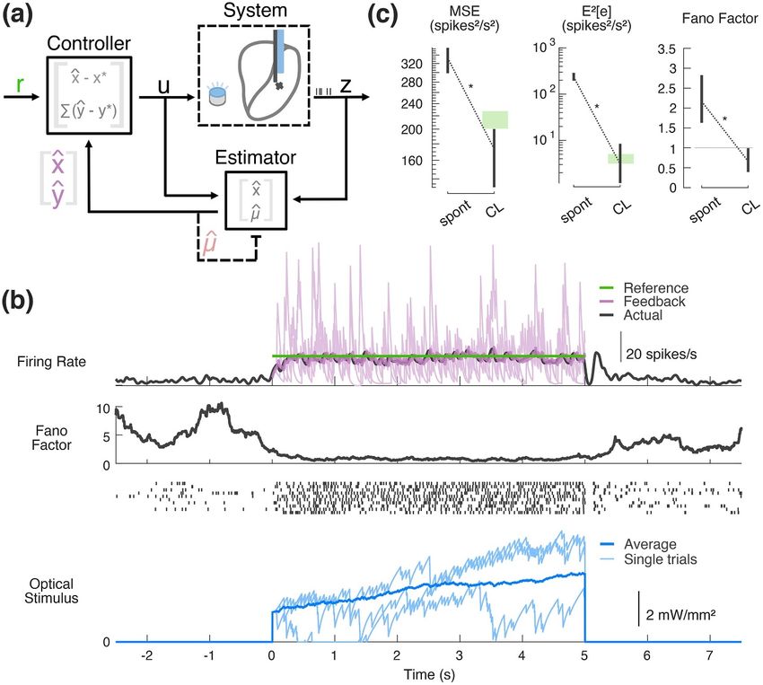
Figure 1. Closed-loop optogenetic control using state-space linear dynamical systems models. (a) Experimental setup. (b)
Control system block flow diagram. Spiking activity is fed back to a model-based estimator (‘EST’), which provides online
estimates of the underlying state of the system (x) and the output (y), which is firing rate in the current application. The
controller (‘CTRL’) uses a model to generate the system setpoint [y∗⊤ x∗⊤ u∗⊤ ]⊤ that corresponds to user-specified reference
firing rate (r). An updated control signal is generated using feedback controller gains and the error between this setpoint and the
online estimates of the system state/output. The updated control signal is sent to an LED driver to modulate light intensity. (c)
Structure of the Gaussian LDS Model. The GLDS used throughout the control loop consists of a linear dynamical system (LDS)
describing the evolution of the state (x) and a linear remapping of x to the output firing rate and eventually measured spiking (z).
This model is used for single-neuron and multi-neuron estimation/control. (d) Workflow for closed-loop experiments. Neuronal
responses to optical noise recorded in previous experiments (left) were used to fit state-space models and design the control
system (middle). The resulting model-based control system was used in subsequent CL control experiments (right).
excluded other thalamic neurons that exhibited more the raw 1 ms PSTH explained by 5th order PLDS and
heterogeneous behaviour (i.e. a minority of recor- GLDS fits (pVE). Note that a relatively low proportion
ded neurons were indirectly inhibited by the optical of the variance in the raw PSTHs was explained, due
input, interestingly). To capture the full heterogeneity to levels of intrinsic noise in the observed responses at
of the population, therefore, we fit 5th order PLDS fine timescales. For this reason, we assessed the qual-
and GLDS models to each single-output dataset indi- ity of the model using a metric that takes into account
vidually (n = 48 neurons, 17 recordings in 9 mice). the fact that some of the observed variability is not
A representative example SISO dataset is shown in explainable across trials [27], instead quantifying the
figure 2(c), where the firing rate estimates for the 5th amount of explainable, or ‘signal’, variance the model
order PLDS (first row, orange) and 5th order GLDS captures. The right panel of figure 2(d) presents the
(second row, red) are superimposed onto the corres- proportion of the signal variance explained (pSVE),
ponding PSTH (black) at white-noise onset and off- showing that the models captured approximately 60%
set. Qualitatively, there is little gained in using a PLDS of the explainable variance and that there was not
model instead of a GLDS for this example, aside from a significant difference in the predictive capabilities
the non-negativity of the PLDS firing rate. Across the between the GLDS and the PLDS models in this data-
population of units, there is no significant difference set. Therefore, with the exception of multi-output
between the performance of the Poisson vs. Gaussian modeling where the same PLDS versus GLDS ana-
models (figure 2(d), n = 48 neurons, p = 0.234, Wil- lysis was conducted for comparison, GLDS models
coxon signed-rank test). Specifically, the left plot of are used for the remainder of this study in order to
figure 2(d) shows the proportion of the variance in leverage linear controls approaches.
9J. Neural Eng. 18 (2021) 036006 M F Bolus et al
Figure 2. State-space models of SISO optogenetic responses. (a) SISO LDS model structure: Poisson (top) or Gaussian (bottom)
output functions being considered. (b) Population impulse response. This impulse response was fit using pooled data from 37
neurons that were excited by optical noise. An FIR model fit to population data (black) is plotted alongside the impulse response
from the 5th order GLDS model fit to the same data (red). (c) Example Data and Model Fits. Top, the PSTH (black) was
smoothed with a 1 ms standard deviation Gaussian window for visualization. The fit types include 5th-order PLDS (orange),
5th-order GLDS (red). Middle, the corresponding trial-by-trial spike raster. Bottom, repeated instantiation of uniform optical
noise. (d) Proportion variance in PSTH explained (pVE) and signal variance explained (pSVE) by model response to noise. All
models were trained on data from first half of each trial, while model performance metrics (pVE, pSVE) were calculated from the
second half of each trial. Error bars represent bootstrapped 95% confidence intervals about the population mean (n = 48
neurons, 17 recordings, 9 animals).
3.2. Parameter-adaptive Kalman filtering provides stimulation and then consistently underestimates the
robust online estimation firing rate at steady state. Model-based control and
These GLDS models are used online as part of the estimation schemes are particularly sensitive to such
Kalman-filter-based estimator (figure 3(a), grey box) plant-model mismatch, as is apparent here when
which is used to provide state feedback to the con- standard Kalman filtering used for online estima-
troller. While the models performed relatively well tion is applied to these datasets for step changes in
in the case of uniform white-noise optical stimula- input. In this example in figure 3(b) there is still
tion as shown in figure 2, when challenged with step an obvious bias in the average Kalman-filter estim-
changes in input that are often utilized in control ated firing rate (KF Estimate, purple) when compared
scenarios, non-zero-mean model mismatch is clearly to the smoothed PSTH (PSTH, black). Moreover,
revealed (figure 3(b)). In this example the open-loop because of the rapid time-course of the fit neuronal
model predicted firing rate (OL Prediction, red) ini- dynamics (figure 2(b)) and the spiking nature of the
tially under-estimates the experimentally-measured measurements, the single-trial KF estimates of firing
firing rate (PSTH, black) during the first second of rate which will be fed back to a controller are full
10J. Neural Eng. 18 (2021) 036006 M F Bolus et al
of extreme transients each time a new spike is meas- previous experiments in separate mice, as illustrated
ured (figure 3(c), purple trace). Online estimation in figure 1(d). As previously noted, 1st-order GLDS
of firing rate can be made more robust by assum- models were sufficient and were therefore used for
ing there is an unmeasured, non-zero-mean disturb- this particular application; however, higher order
ance that varies stochastically (e.g. other exogenous models would be merited or necessary in other scen-
inputs), augmenting the state with the mean(s) of this arios. The robustness of the estimator (figure 3), the
disturbance (µ), and jointly re-estimating this along use of feedback, and the slow timescale nature of the
with the state using Kalman filtering (figure 3(d), control objective allowed GLDS models fit to pre-
see methods for details), which we refer to here as viously collected noise response data to be used for
the parameter-adaptive Kalman filter, but has else- experimental control and estimation, rather than fit-
where been described as a proportional-integral Kal- ting a model during an experiment, the timespan of
man filter [34, 35]. As can be seen in the example in which is limited in the context of awake, head-fixed
figure 3(e), this adaptive Kalman filter produces an recordings. The feedback controller was designed
effectively unbiased estimate of the experimentally- using output-weighted LQR [37], where the state of
observed PSTH in SISO applications (figure 3(e), the system was augmented with the integrated output
purple vs. black), and it is able to do so with a single- in order to find not only proportional feedback gains
trial estimate of firing rate that is smoother than that on the state, but integral feedback gains to minimize
achieved by the standard Kalman filter (figure 3(f), cf. steady state tracking errors (section 2.6.2). Addition-
figure 3(c)). In this example, the parameter-adaptive ally, since this particular application is a non-zero set-
Kalman filter approach accounts for apparent model point regulation problem, the steady-state set-point
⊤
mismatch by estimating a process disturbance µ that of the system y∗⊤ x∗⊤ u∗⊤ at the desired out-
on average pushes the firing rate above the model put firing rate (r) was calculated as described in
prediction for the first second of optical stimulation section 2.6.1.
and then pulls the estimated firing rate below that Figure 4 illustrates the performance of the con-
prediction at steady state (figure 3(g)). The filtering trol framework for a typical single thalamic neuron
approach works well in this illustrative example and and the summary performance across experiments.
at a population level, as it brings the estimation bias Figure 4(a) is an illustration of the control imple-
to near-zero levels compared to the standard Kalman mentation, highlighting the feedback controller and
filter (figure 3(h), p = 1.63 × 10⁻⁹ , Wilcoxon signed- the online estimator. In the case of the estimator,
rank test, n = 48 neurons, 17 experiments, 9 animals). Parameter-adaptive Kalman filtering is being used
At least in the context of estimating step responses, we to estimate not only the state of the system being
see there is little benefit in using a 5th order versus controlled but also the uncontrolled disturbance
1st-order GLDS model for this SISO application (figure 4(a), estimator block). On the other hand,
(figure 3(h), black, p = 0.083 0, Wilcoxon signed-rank the controller is operating on the error between the
test). Importantly, the parameter adaptation provides estimated state of the system and the desired steady-
enough robustness that even the population-average state set point as well as the integrated output error
GLDS model in figure 2(b) was able to estimate SISO (figure 4(a), controller block). In this example (figure
firing nearly as well as models fit to each neuron 4(b)), the baseline ongoing activity of the recor-
individually (figure 3(h), gray, p = 0.014 2, Wilcoxon ded neuron was approximately 5 spikes s−1 , and
signed-rank test). Since the control objective in this the controller was activated at time zero with a tar-
study is to clamp firing rate at relatively long times- get firing rate of 20 spikes s−1 . Upon activating the
cales, we therefore used a 1st-order Gaussian approx- controller, the neuron reached and remained at the
imation for the system. However, for fast timescale target firing rate (green), as reflected in the aver-
trajectory tracking problems, a higher-order model age firing rate (black). Importantly, the controller
would almost certainly be warranted (see Discus- operated using online estimates of state and corres-
sion), and higher-order models are important even ponding output firing rate provided by the estim-
for long timescale control/estimation in multi-output ator (figure 4(b), purple). The firing rate of the
scenarios (see section 3.6). online estimator (purple) also quickly reached the
target (green) and remained there. As shown previ-
3.3. State-space control performs well in SISO ously in figure 3, the online estimate was on aver-
clamping applications age unbiased, as it matched the offline estimate of
The control and estimation framework was tested the average firing (black, PSTH smoothed with 25 ms
experimentally in the awake head-fixed mouse in s.d. Gaussian). The controller achieved the target
a SISO configuration, where spiking activity of a with well-below spontaneous levels of across-trial
single neuron was fed back to a controller with a variability, quantified using the Fano factor (FF) that
single channel of optical input. The models used captures the spike count variance relative to the mean
for pre-experiment controller design and for the spike count (figure 4(b), middle). In this particular
online estimation for state feedback were fit to example, the controller’s use of feedback resulted in a
thalamic spiking responses to optical noise from gradual increase in light intensity that was needed to
11J. Neural Eng. 18 (2021) 036006 M F Bolus et al
Figure 3. Kalman filtering for online estimation in SISO applications. (a) Standard Kalman filter. Prediction error (e) is used to
correct the estimate of state at each time step. (b) Example open-loop (OL) prediction of neuronal response (red) to step input of
light (blue) using 5th order GLDS fit to noise-driven data, compared to PSTH smoothed with 25 ms Gaussian window (black)
and the trial-averaged response estimated using the standard implementation of the Kalman filter (5th-order GLDS) (purple). (c)
Example single-trial Kalman filter estimate (purple) along with corresponding spike raster (grey). (d) Parameter-adaptive Kalman
filter. In addition to estimating the state of the system, this approach jointly re-estimates a state disturbance (µ) at each time step.
(e) Same as (b) but trial-averaged estimate of firing rate using the parameter-adaptive Kalman filter. (f) Same as (c) except
single-trial estimate using parameter-adaptive Kalman filter. (g) Trial-averaged disturbance on the first state estimated using
parameter-adaptive Kalman filter. (h) Population average squared-bias in estimation calculated between the single-trial spiking
responses and the OL prediction of a 5th-order GLDS, the standard Kalman filter using the 5th-order GLDS, and the
parameter-adaptive Kalman filter (aKF) using a 1st- or 5th-order GLDS. Black and grey data points correspond to error
associated with using individually-fit models vs. a single population average fit model, respectively. Error bars represent
bootstrapped 95% confidence intervals about the mean (n = 48 neurons, 17 recordings, 9 animals).
maintain the target level of spiking over the control in figure 4(c). For each of these metrics, the meas-
epoch. Also note that this control signal varied sub- ure during closed-loop (CL) control is compared to
stantially across individual trials (figure 4(b), bottom, that from the spontaneous period (spont) before the
light blue), with significant individual trial variability control was activated at time zero. The mean squared-
serving to drive the firing rate tracking and quench error (MSE) between an offline estimate of the single-
the variability. While variable across experiments, in trial firing rate and the target (figure 4(c) left)
general it was approximately 1.1 seconds before the decreased significantly with activation of the control
controller was able to push neuronal firing to within law as expected (p = 0.001 95, Wilcoxon signed-rank
2% of its steady state value (bootstrapped 95% con- test), and the MSE during closed-loop control was
fidence intervals about the median, 0.47–1.34 s, n = even below that of a Poisson spike generator driven
11 recordings). This settling time metric was calcu- at the target rate (green bar), consistent with the sub-
lated by fitting a second order transfer function to Poisson variability as revealed by the Fano-factor in
closed-loop step data and using the MATLAB ‘step- figure 4(b). Because the MSE captures a combina-
info’ function (Mathworks, Inc.). tion of the variance and the bias, we separately com-
Across experiments (n = 11 neurons, 11 exper- puted the bias in the control (figure 4(c) middle),
iments), the control framework performed well as substantially reduced with the activation of the con-
quantified by the summary of performance metrics trol (p = 0.000 977, Wilcoxon signed-rank test) and
12J. Neural Eng. 18 (2021) 036006 M F Bolus et al
Figure 4. Experimental SISO control and estimation. (a) SISO control block flow diagram. Shown inside the controller and
estimator blocks are the notions of state being used in each operation. (b) Example experimental SISO control. (top) Fed-back
online estimate in purple (single trial in light purple, trial-averaged in bold), along with the corresponding trial-average offline
estimate (25 ms s.d. Gaussian-smoothed PSTH); (middle) across-trial spike count variability (Fano factor in 500 ms sliding
window) and corresponding example spike rasters from 10 randomly selected trials; (bottom) controller input. (c) Population
controller performance. In spontaneous vs. closed-loop (CL) control conditions, mean squared error (left) and squared bias
(middle) were calculated between the reference (20 spikes s−1 ) and single-trial feedback spiking data smoothed with a 25 ms s.d.
Gaussian window; average Fano factor was also calculated (right). For each trial, four seconds of spontaneous data were
compared to four seconds of CL control data. The first second was ignored in order to obtain a measure of steady-state
performance. Error bars represent bootstrapped 95% confidence intervals about the mean. Green bands represent 95%
confidence band for the metrics calculated from simulated Poisson firing at the target rate.
at the level expected for a Poisson spike generator one of the main benefits of using state-space mod-
driven at the target rate (green band). To further els for control and estimation is the generalizabil-
quantify the reduction in across-trial variability dur- ity to such multi-output problems. While the pre-
ing the control, we computed the average Fano-factor ceding experimental demonstration was presented in
in a 500 ms sliding window, exhibiting substantial the context of a single channel of light input and
reduction from supra-Poisson variability (FF> 1) in a single channel of neuronal output, in a subset of
the spontaneous activity to sub-Poisson variability experiments, we simultaneously recorded multiple
(FF< 1) during the control (figure 4(c) right). nearby neurons in the thalamus of the awake, head-
fixed mouse. This provides a window into the effect
3.4. Multi-electrode recordings reveal effects of of the stimulation on the local population while a
SISO control on simultaneously recorded neurons single neuron is used as an ‘antenna’ around which
Up to this point, the state-space control framework the controller is operating, which we will refer to as
has been shown effective for tracking step commands the feedback (FB) neuron (figure 5(a)). For the pur-
in single-neuron scenarios. However, neural record- poses of this analysis, we inspected simultaneously-
ing methodologies (electrophysiology and imaging) recorded neurons that were excited by 5 ms square
continue to scale in size (e.g. larger numbers of chan- pulses of light with sub-10 ms latency. Figure 5(b)
nels for electrophysiology, or pixels for imaging) and provides an example in which one neuron is being
13You can also read