House Prices, Credit Growth, and Excess Volatility: Implications for Monetary and Macroprudential Policy
←
→
Page content transcription
If your browser does not render page correctly, please read the page content below
House Prices, Credit Growth, and Excess
       Volatility: Implications for Monetary and
                Macroprudential Policy∗

 Paolo Gelain,a Kevin J. Lansing,a,b and Caterina Mendicinoc
                                 a
                                   Norges Bank
                  b
                      Federal Reserve Bank of San Francisco
                               c
                                 Bank of Portugal

           Progress on the question of whether policymakers should
       respond directly to financial variables requires a realistic eco-
       nomic model that captures the links between asset prices,
       credit expansion, and real economic activity. Standard DSGE
       models with fully rational expectations have difficulty pro-
       ducing large swings in house prices and household debt that
       resemble the patterns observed in many industrial countries
       over the past decade. We show that the introduction of sim-
       ple moving-average forecast rules for a subset of agents can
       significantly magnify the volatility and persistence of house
       prices and household debt relative to an otherwise similar
       model with fully rational expectations. We evaluate various

   ∗
     For helpful comments and suggestions, we would like to thank Kim Abild-
gren, Pierpaolo Benigno, Allesandro Notarpietro, Kjetil Olsen, Bruce Preston,
Vincenzo Quadrini, Øistein Røisland, Federico Signoretti, Anders Vredin, semi-
nar participants at the Bank of Canada, the Norges Bank Macro-Finance Forum,
Sveriges Riksbank, Swiss National Bank, the 2012 Meeting of the International
Finance and Banking Society, the 2012 Meeting of the Society for Computa-
tional Economics, the 2012 ESCB Day-Ahead Conference in Malaga, the 2012
Central Bank Modeling Workshop hosted by the National Bank of Poland, the
2012 Dynare Conference, the 2012 Fall Conference of the International Jour-
nal of Central Banking hosted by the Central Bank of Chile, the 2012 Central
Bank of Turkey conference on “Reserve Requirements and Other Macropruden-
tial Policies,” the 2012 Second Conference of the ESCB Macroprudential Research
Network hosted by the European Central Bank, and the 2013 UCLA/FRB-San
Francisco Conference on Housing and the Macroeconomy. Corresponding author
(Lansing): Federal Reserve Bank of San Francisco, P.O. Box 7702, San Fran-
cisco, CA 94120-7702, e-mail: kevin.j.lansing@sf.frb.org or kevin.lansing@norges-
bank.no.

                                      219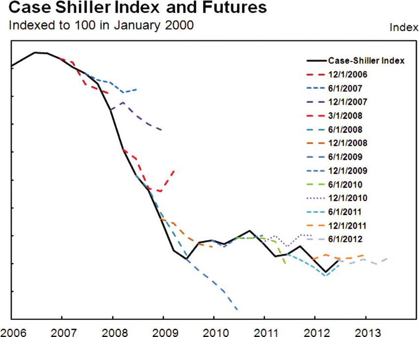
220           International Journal of Central Banking                June 2013

       policy actions that might be used to dampen the resulting
       excess volatility, including a direct response to house-price
       growth or credit growth in the central bank’s interest rate rule,
       the imposition of a more restrictive loan-to-value ratio, and the
       use of a modified collateral constraint that takes into account
       the borrower’s wage income. Of these, we find that a debt-to-
       income type constraint is the most effective tool for dampening
       overall excess volatility in the model economy. While an inter-
       est rate response to house-price growth or credit growth can
       stabilize some economic variables, it can significantly magnify
       the volatility of others, particularly inflation.
       JEL Codes: D84, E32, E44, G12, O40.

1.    Introduction

Household leverage in many industrial countries increased dramati-
cally in the years prior to 2007. Countries with the largest increases
in household debt relative to income tended to experience the fastest
run-ups in house prices over the same period. The same countries
tended to experience the most severe declines in consumption once
house prices started falling (Glick and Lansing 2010; International
Monetary Fund 2012).1 Within the United States, house prices dur-
ing the boom years of the mid-2000s rose faster in areas where sub-
prime and exotic mortgages were more prevalent (Tal 2006; Mian
and Sufi 2009; Pavlov and Wachter 2011). In a given area, past
house-price appreciation had a significant positive influence on sub-
sequent loan approval rates (Dell’Ariccia, Igan, and Laeven 2012;
Goetzmann, Peng, and Yen 2012). Areas in the United States which
experienced the largest run-ups in household leverage tended to
experience the most severe recessions as measured by the subsequent
fall in durables consumption or the subsequent rise in the unemploy-
ment rate (Mian and Sufi 2010). Recession severity in a given area

   1
     King (1994) identified a similar correlation between prior increases in house-
hold debt ratios and the severity of the early 1990s recession using data for ten
major industrial countries from 1984 to 1992. King also notes that U.S. consumer
debt more than doubled during the 1920s—a factor that likely contributed to the
severity of the Great Depression in the early 1930s.
Vol. 9 No. 2 House Prices, Credit Growth, and Excess Volatility 221
appears to reflect the degree to which prior growth in that area
was driven by an unsustainable borrowing trend—one which came
to an abrupt halt once house prices stopped rising (Mian and Sufi
2012). Overall, the data suggests the presence of a self-reinforcing
feedback loop in which an influx of new homebuyers with access to
easy mortgage credit helped fuel an excessive run-up in house prices.
The run-up, in turn, encouraged lenders to ease credit further on the
assumption that house prices would continue to rise.
Figure 1 illustrates the simultaneous boom in U.S. real house
prices and per capita real household debt that occurred during the
mid-2000s. During the boom years, per capita real GDP remained
consistently above trend. A common feature of all bubbles which
complicates the job of policymakers is the emergence of seemingly
plausible fundamental arguments that seek to justify the dramatic
rise in asset prices. The U.S. housing boom was no different. During
the boom years, many economists and policymakers argued that a
bubble did not exist and that numerous fundamental factors, includ-
ing the strength of the U.S. economy, were driving the run-up in
prices.2 But in retrospect, many studies now attribute the run-up
to a classic bubble driven by overoptimistic projections about future
house-price growth which, in turn, led to a collapse in lending stan-
dards.3 Reminiscent of the U.S. stock market mania of the late-
1990s, the mid-2000s housing market was characterized by an influx
of unsophisticated buyers and record transaction volume. When the
2
See, for example, McCarthy and Peach (2004) and Himmelberg, Mayer,
and Sinai (2005). In an October 2004 speech, Federal Reserve Chairman Alan
Greenspan (2004a) argued that there were “significant impediments to specula-
tive trading” in the housing market that served as “an important restraint on the
development of price bubbles.” In a July 1, 2005 media interview, Ben Bernanke,
then Chairman of the President’s Council of Economic Advisers, asserted that
fundamental factors such as strong growth in jobs and incomes, low mortgage
rates, demographics, and restricted supply were supporting U.S. house prices.
In the same interview, Bernanke stated his view that a substantial nationwide
decline in house prices was “a pretty unlikely possibility.” For additional details,
see Jurgilas and Lansing (2013).
3
For a comprehensive review of events, see the report of the U.S. Financial
Crisis Inquiry Commission (2011). Recently, in a review of the Federal Reserve’s
forecasting record leading up to the crisis, Potter (2011) acknowledges a “misun-
derstanding of the housing boom . . . [which] downplayed the risk of a substantial
fall in house prices” and a “lack of analysis of the rapid growth of new forms of
mortgage finance.”222 International Journal of Central Banking June 2013
Figure 1. U.S. Real House Prices, Real Household Debt,
and Real GDP
U.S. real house prices (in logs) U.S. real house prices
20
% deviation from trend
10
0.4
0
0.2 Linear trend −10
−20
1990 1995 2000 2005 2010 1990 1995 2000 2005 2010
U.S. real household debt per capita (in logs) U.S. real household debt per capita
2 40
% deviation from trend
1.5 20
1 0
Linear trend
0.5 −20
1990 1995 2000 2005 2010 1990 1995 2000 2005 2010
U.S. real GDP per capita (in logs) U.S. real GDP per capita
1 10
% deviation from trend
0.8 5
0.6 0
0.4 Linear trend −5
0.2 −10
1990 1995 2000 2005 2010 1990 1995 2000 2005 2010
Notes: U.S. real house prices (from U.S. Census Bureau) and real household
debt (from Federal Reserve Flow of Funds) both increased dramatically starting
around the year 2000. During the boom years, per capita real GDP remained
consistently above trend. House prices have since retraced to the downside, while
the level of household debt has declined slightly. Real GDP experienced a sharp
drop during the Great Recession and remains about 5 percent below trend.
optimistic house-price projections eventually failed to materialize,
the bubble burst, setting off a chain of events that led to a finan-
cial and economic crisis. The “Great Recession,” which started in
December 2007 and ended in June 2009, was the most severe eco-
nomic contraction since 1947, as measured by the peak-to-trough
decline in real GDP.
Much of the strength of the U.S. economy during the mid-2000s
was linked to the housing boom itself. Consumers extracted equityVol. 9 No. 2 House Prices, Credit Growth, and Excess Volatility 223
from appreciating home values to pay for all kinds of goods and
services while hundreds of thousands of jobs were created in resi-
dential construction, mortgage banking, and real estate. After peak-
ing in 2006, real house prices have retraced to the downside while
the level of real household debt has started to decline. Real GDP
experienced a sharp drop during the Great Recession and remains
about 5 percent below trend. Other macroeconomic variables also
suffered severe declines, including per capita real consumption and
the employment-to-population ratio.4
Nearly four years after the end of the Great Recession, the
unwinding of excess household leverage is still imposing a signifi-
cant drag on consumer spending and bank lending in many coun-
tries, thus hindering the vigor of the global economic recovery.5 In
the aftermath of the global financial crisis and the Great Reces-
sion, it is important to consider what lessons might be learned for
the conduct of policy. Historical episodes of sustained rapid credit
expansion together with booming stock or house prices have often
signaled threats to financial and economic stability (Borio and Lowe
2002). Times of prosperity which are fueled by easy credit and
rising debt are typically followed by lengthy periods of deleverag-
ing and subdued growth in GDP and employment (Reinhart and
Reinhart 2010). As noted originally by Persons (1930), “When the
process of expanding credit ceases and we return to a normal basis
of spending each year . . . there must ensue a painful period of
readjustment.” According to Borio and Lowe (2002), “If the econ-
omy is indeed robust and the boom is sustainable, actions by the
authorities to restrain the boom are unlikely to derail it altogether.
By contrast, failure to act could have much more damaging conse-
quences, as the imbalances unravel.” This raises the question of what
“actions by the authorities” could be used to restrain the boom?
Our aim in this paper is to explore the effects of various policy
measures that might be used to lean against credit-fueled financial
imbalances.
Standard dynamic stochastic general equilibrium (DSGE) mod-
els with fully rational expectations have difficulty producing large
swings in house prices and household debt that resemble the patterns
4
For details, see Lansing (2011).
5
See, for example, Roxburgh et al. (2012).224 International Journal of Central Banking June 2013
observed in many industrial countries over the past decade. Indeed,
it is common for such models to include extremely large and persis-
tent exogenous shocks to rational agents’ preferences for housing in
an effort to bridge the gap between the model and the data.6 Leaving
aside questions about where these preference shocks actually come
from and how agents’ responses to them could become coordinated,
if housing booms and busts were truly driven by preference shocks,
then central banks would seem to have little reason to be concerned
about them. Declines in the collateral value of an asset are often
modeled as being driven by exogenous fundamental shocks to the
“quality” of the asset, rather than the result of a burst asset-price
bubble.7 Taken literally, this type of model would imply that the
decline in U.S. house prices since 2007 was caused by something akin
to a nationwide infestation of wood termites. Kocherlakota (2010)
remarks: “The sources of disturbances in macroeconomic models are
(to my taste) patently unrealistic. . . . I believe that [macroecono-
mists] are handicapping themselves by only looking at shocks to
fundamentals like preferences and technology. Phenomena like credit
market crunches or asset market bubbles rely on self-fulfilling beliefs
about what others will do.” These ideas motivate consideration of
a model where agents’ subjective forecasts serve as an endogenous
source of volatility.
We use the term “excess volatility” to describe a situation where
asset prices and macroeconomic variables move too much to be
explained by a rational response to fundamentals. Numerous empiri-
cal studies starting with LeRoy and Porter (1981) and Shiller (1981)
have shown that stock prices appear to exhibit excess volatility when
compared with the discounted stream of ex post realized dividends.8
6
Examples include Iacoviello (2005), Iacoviello and Neri (2010), Walentin and
Sellin (2010), Lambertini, Mendicino, and Punzi (2011), and Kannan, Rabanal,
and Scott (2012), among others.
7
See, for example, Gertler, Kiyotaki, and Queralto (2012) in which a financial
crisis is triggered by an exogenous “disaster shock” that wipes out a fraction
of the productive capital stock. Similarly, a model-based study by the Interna-
tional Monetary Fund (2009, p. 110) acknowledges that “although asset booms
can arise from expectations . . . without any change in fundamentals, we do not
model bubbles or irrational exuberence.” Gilchrist and Leahy (2002) examine the
response of monetary policy to asset prices in a rational expectations model with
exogenous “net worth shocks.”
8
Lansing and LeRoy (2012) provide a recent update on this literature.Vol. 9 No. 2 House Prices, Credit Growth, and Excess Volatility 225
Similarly, Campbell et al. (2009) find that movements in U.S. house
price-rent ratios cannot be fully explained by movements in future
rent growth.
We introduce excess volatility into an otherwise standard DSGE
model by allowing a fraction of households to employ simple moving-
average forecast rules, i.e., adaptive expectations. Following the
asset-pricing literature, excess volatility is measured relative to the
fluctuations generated by the same model under fully rational expec-
tations. We show that the use of moving-average forecast rules by
a subset of agents can significantly magnify the volatility and per-
sistence of house prices and household debt. The moving-average
forecast rule embeds a unit-root assumption which tends to be par-
tially self-fulfilling. As shown originally by Muth (1960), a moving-
average forecast rule with exponentially declining weights on past
data will coincide with rational expectations when the forecast vari-
able evolves as a random walk with permanent and temporary
shocks. But even if this is not the case, a moving-average forecast rule
can be viewed as boundedly rational because it economizes on the
costs of collecting and processing information. As noted by Nerlove
(1983, p. 1255), “Purposeful economic agents have incentives to elim-
inate errors up to a point justified by the costs of obtaining the
information necessary to do so. . . . The most readily available and
least costly information about the future value of a variable is its
past value.”
The basic structure of the model is similar to Iacoviello (2005)
with two types of households. Patient-lender households own the
entire capital stock and operate monopolistically competitive firms.
Our setup roughly approximates the highly skewed distribution of
U.S. financial wealth in which the top decile of households own about
80 percent of financial wealth. Impatient-borrower households derive
income only from labor and face a borrowing constraint linked to
the market value of their housing stock. Expectations are modeled
as a weighted average of a fully rational forecast rule and a moving-
average forecast rule. We calibrate the parameters of the hybrid
expectations model to generate an empirically plausible degree of
volatility in the simulated house price, household debt, and real
output series. Our calibration implies that 30 percent of house-
holds employ a moving-average forecast rule, while the remaining 70226 International Journal of Central Banking June 2013
percent are fully rational.9 Due to the self-referential nature of the
model’s equilibrium conditions, the unit-root assumption embedded
in the moving-average forecast rule serves to magnify the volatility of
endogenous variables in the model. Our setup captures the idea that
much of the run-up in U.S. house prices and credit during the boom
years was linked to the influx of an unsophisticated population of
new homebuyers.10 Given their inexperience, these buyers would be
more likely to employ simple forecast rules for future house prices,
income, etc. One can also make the case that many U.S. lenders
behaved similarly by approving loans that could only be repaid if
house prices continued to trend upward indefinitely.
Survey data from both stock and real estate markets provides
strong empirical support for considering extrapolative or moving-
average type forecast rules.11 In a comprehensive study of the expec-
tations of U.S. stock market investors using survey data from a vari-
ety of sources, Greenwood and Shleifer (2013) find that measures of
investor expectations about future stock returns are positively corre-
lated with past stock returns and investor inflows into mutual funds.
They conclude (p. 30) that “our evidence rules out rational expec-
tations models in which changes in market valuations are driven by
the required returns of a representative investor. . . . Future mod-
els of stock market fluctuations should embrace the large fraction
of investors whose expectations are extrapolative.” We apply their
advice in the present paper to a model of house-price fluctuations.
Case, Shiller, and Thompson (2012) perform an analysis of sur-
vey data on people’s house-price expectations in four cities over the
period 2003 to 2012. They report (p. 17) that “12-month expecta-
tions [of house price changes] are fairly well described as attenuated
versions of lagged actual 12-month price changes.” Figure 2 shows
that house-price forecasts derived from the futures market for the
Case-Shiller house-price index (which are only available from 2006
onwards) typically exhibit a sustained series of one-sided forecast
9
Using U.S. data over the period 1981 to 2006, Levine et al. (2012) estimate
that around 65 to 80 percent of agents employ moving-average forecast rules in
the context of a DSGE model which omits house prices and household debt.
10
See Mian and Sufi (2009) and chapter 6 of the report of the U.S. Financial
Crisis Inquiry Commission (2011), titled “Credit Expansion.”
11
For a summary of the evidence, see Jurgilas and Lansing (2013).Vol. 9 No. 2 House Prices, Credit Growth, and Excess Volatility 227
Figure 2. Futures Market Forecasts for U.S. House Prices
Notes: Futures market forecasts for house prices tend to overpredict subse-
quent actual house prices when prices are falling—a pattern consistent with a
moving-average forecast rule.
Source: Bloomberg.
errors. The futures market tends to overpredict future house prices
when prices are falling—a pattern that is consistent with a moving-
average forecast rule. Similarly, the top panel of figure 3 shows that
U.S. inflation expectations derived from the Survey of Professional
Forecasters tend to systematically underpredict subsequent actual
inflation in the sample period prior to 1979 when inflation was rising
and systematically overpredict actual inflation thereafter when infla-
tion was falling. Rational expectations would not give rise to such a
sustained sequence of one-sided forecast errors.12 The bottom panel
12
Numerous studies document evidence of bias and inefficiency in survey fore-
casts of U.S. inflation. See, for example, Roberts (1997), Mehra (2002), Carroll
(2003), and Mankiw, Reis, and Wolfers (2004). More recently, Coibion and Gorod-
nichencko (2012) find robust evidence against full-information rational expecta-
tions in survey forecasts for U.S. inflation and unemployment. Fuhrer (2012)
estimates “a small and economically insignificant role for rational expectations
and lagged dependent variables . . . once the information in survey expectations
is taken into account.”228 International Journal of Central Banking June 2013
Figure 3. Inflation Expectations from the Survey of
Professional Forecasters
Notes: U.S. inflation expectations derived from the Survey of Professional Fore-
casters (SPF) tend to systematically underpredict subsequent actual inflation
in the sample period prior to 1979 when inflation was rising and systematically
overpredict it thereafter when inflation was falling. The survey pattern is well
captured by the moving average of past inflation rates.
of figure 3 shows that the survey pattern of professional forecasters
is well captured by an exponentially weighted moving average of
past inflation rates, where the weight λ on the most recent infla-
tion observation is 0.35. Interestingly, a weight of 0.35 on the most
recent inflation observation is consistent with a Kalman-filter fore-
cast in which the forecasters’ perceived law of motion for inflation
is a random walk plus noise (Lansing 2009).
The volatilities of house prices and household debt in the hybrid
expectations model are around 1.5 times larger than those in the
rational expectations model. Moreover, both variables exhibit sig-
nificantly higher persistence under hybrid expectations. Stock-priceVol. 9 No. 2 House Prices, Credit Growth, and Excess Volatility 229
volatility is magnified by a factor of about 1.4, whereas the volatili-
ties of output, inflation, consumption, and labor hours are magnified
by factors ranging from about 1.2 to 1.4. These results are strik-
ing given that only 30 percent of households in the model employ
moving-average forecast rules. The use of such forecast rules by even
a small subset of agents can have a large influence on model dynam-
ics because the presence of these agents influences the nature of the
fully rational forecast rules employed by the remaining agents.
Given the presence of excess volatility, we evaluate various pol-
icy actions that might be used to dampen the observed fluctuations.
With regard to monetary policy, we consider a direct response to
either house-price growth or credit growth in the central bank’s
interest rate rule. With regard to macroprudential policy, we con-
sider the imposition of a more restrictive loan-to-value ratio (i.e., a
tightening of lending standards) and the use of a modified collat-
eral constraint that takes into account the borrower’s wage income.
Of these, we find that a debt-to-income type constraint is the most
effective tool for dampening overall excess volatility in the model
economy. We find that while an interest rate response to house-price
growth or credit growth can stabilize some economic variables, it can
significantly magnify the volatility of others, particularly inflation.
Our results for an interest rate response to house-price growth
show some benefits under rational expectations (lower volatilities
for household debt, stock prices, and consumption), but the bene-
fits under hybrid expectations are more limited (lower volatility for
household debt). Under both expectation regimes, inflation volatility
is magnified, with the effect being more severe under hybrid expec-
tations. Such results are unsatisfactory from the standpoint of an
inflation-targeting central bank that seeks to minimize a weighted
sum of squared deviations of inflation and output from target values.
Indeed we show that the value of a typical central bank loss function
rises monotonically as more weight in placed on house-price growth
in the interest rate rule.
The results for an interest rate response to credit growth also
show some benefits under rational expectations. However, these ben-
efits completely disappear under hybrid expectations. Moreover, the
undesirable magnification of inflation volatility becomes much worse.
The results for this experiment demonstrate that the effects of a par-
ticular monetary policy can be influenced by the nature of agents’230 International Journal of Central Banking June 2013
expectations.13 We note that Christiano et al. (2010) find that a
strong interest rate response to credit growth can improve the wel-
fare of a representative household in a rational expectations model
with news shocks. Kannan, Rabanal, and Scott (2012) find that an
interest rate response to credit growth can help reduce the value of
a central bank loss function in a rational expectations model with
large and persistent housing preference shocks. Both of these results
could be sensitive to the assumption that all agents employ fully
rational expectations.
Turning to macroprudential policy, we find that a reduction in
the loan-to-value ratio from 0.7 to 0.5 substantially reduces the
volatility of household debt under both expectations regimes, but
output volatility is slightly magnified. The volatility effects on other
variables are generally small. For policymakers, the mixed stabiliza-
tion results must be weighed against the drawbacks of permanently
restricting household access to borrowed money which helps impa-
tient households smooth their consumption. A natural alternative
to a permanent change in the loan-to-value ratio is to shift the ratio
in a countercyclical manner without changing its steady-state value.
A number of papers have identified stabilization benefits from the
use of countercyclical loan-to-value rules in rational expectations
models.14 Another macroprudential policy approach, examined by
Bianchi and Mendoza (2010), is to employ a procyclical tax on debt
which leans against overborrowing by rational private-sector agents.
Our second macroprudential policy experiment achieves a coun-
tercyclical loan-to-value ratio in a novel way by requiring lenders
to place a substantial weight on the borrower’s wage income in the
borrowing constraint. As the weight on the borrower’s wage income
increases, the generalized borrowing constraint takes on more of the
characteristics of a debt-to-income constraint. Intuitively, a debt-to-
income constraint represents a more prudent lending criterion than
a loan-to-value constraint because income, unlike asset value, is less
subject to distortions from bubble-like movements in asset prices.
13
Orphanides and Williams (2009) make a related point. They find that an
optimal control policy derived under the assumption of perfect knowledge about
the structure of the economy can perform poorly when knowledge is imperfect.
14
See, for example, Angelini, Neri, and Panetta (2011), Christensen and Meh
(2011), Lambertini, Mendicino, and Punzi (2011), and Kannan, Rabanal, and
Scott (2012).Vol. 9 No. 2 House Prices, Credit Growth, and Excess Volatility 231
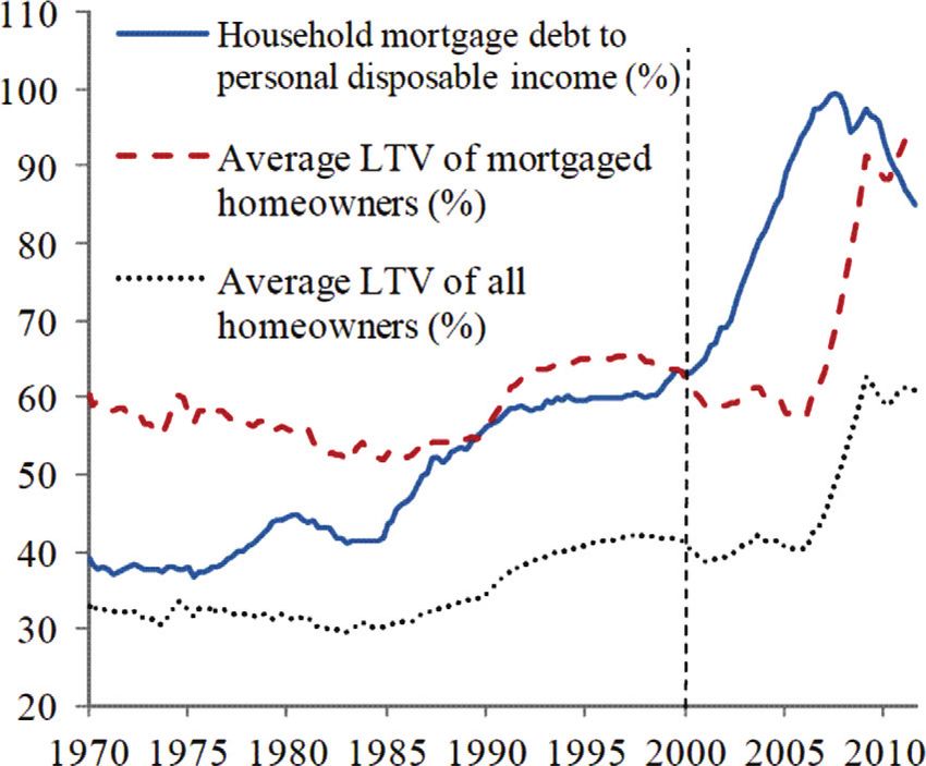
Figure 4. Loan-to-Value Ratios versus Debt-to-Income
Ratio
Notes: During the U.S. housing boom of the mid-2000s, loan-to-value measures
did not signal a significant increase in household leverage, because the value of
housing assets rose together with liabilities in a self-reinforcing feedback loop.
In contrast, the debt-to-income ratio provided regulators with a much earlier
warning signal of the dangerous buildup of household leverage.
Figure 4 shows that during the U.S. housing boom of the mid-2000s,
loan-to-value measures did not signal any significant increase in
household leverage because the value of housing assets rose together
with household mortgage debt in a self-reinforcing feedback loop.
Only after the collapse of house prices did the loan-to-value measures
provide an indication of excessive household leverage. But by then,
the overaccumulation of household debt had already occurred.15 By
contrast, the ratio of household mortgage debt to disposable per-
sonal income started to rise rapidly about five years earlier, providing
regulators with an early warning signal of a potentially dangerous
15
In a February 2004 speech, Federal Reserve Chairman Alan Greenspan
(2004b) remarked, “Overall, the household sector seems to be in good shape,
and much of the apparent increase in the household sector’s debt ratios over
the past decade reflects factors that do not suggest increasing household finan-
cial stress.” Similarly, in an April 2004 speech, Federal Reserve Governor Donald
Kohn (2004) stated, “And, while [household] debt has been increasing, assets on
household balance sheets have been rising even more rapidly.”232 International Journal of Central Banking June 2013
buildup in household leverage. Unfortunately, the signal was not
heeded.
We show that the generalized borrowing constraint serves as an
“automatic stabilizer” by inducing an endogenously countercyclical
loan-to-value ratio. In our view, it is much easier and more real-
istic for regulators to simply mandate a substantial emphasis on
the borrowers’ wage income in the lending decision rather than to
expect regulators to frequently adjust the maximum loan-to-value
ratio in a systematic way over the business cycle or the finan-
cial cycle.16 For the generalized borrowing constraint, we impose
a weight of 75 percent on the borrower’s wage income, with the
remaining 25 percent on the expected value of housing collateral.
The multiplicative parameter in the borrowing constraint is adjusted
to maintain the same steady-state loan-to-value ratio as in the base-
line model. Under hybrid expectations, the generalized borrowing
constraint reduces the volatility of house prices and household debt,
while mildly reducing the volatility of other variables or leaving their
volatility essentially unchanged. Importantly, the policy avoids the
large undesirable magnification of inflation volatility that is observed
in the two interest rate policy experiments.
Comparing across the various policy experiments, the general-
ized borrowing constraint appears to be the most effective tool for
dampening overall excess volatility in the model economy. The value
of a typical central bank loss function declines monotonically (albeit
slightly) as more weight is placed on the borrower’s wage income
in the borrowing constraint. The beneficial stabilization results of
this policy become more dramatic if the loss function is expanded
to take into account the variance of household debt. The expanded
loss function can be interpreted as reflecting a concern for finan-
cial stability. Specifically, the variance of household debt captures
the idea that historical episodes of sustained rapid credit expansion
have often led to crises and severe recessions.17
16
Drehmann, Borio, and Tsatsaronis (2012) employ various methods for dis-
tinguishing the business cycle from the financial or credit cycle. They argue that
the financial cycle is much longer than the traditional business cycle.
17
Akram and Eitrheim (2008) investigate different ways of representing a con-
cern for financial stability in a reduced-form econometric model. Among other
metrics, they consider the standard deviation of the debt-to-income ratio and the
standard deviation of the debt-service-to-income ratio.Vol. 9 No. 2 House Prices, Credit Growth, and Excess Volatility 233
Recently, the Committee on International Economic and Pol-
icy Reform (2011) has called for central banks to go beyond their
traditional emphasis on flexible inflation targeting and adopt an
explicit goal of financial stability. Similarly, Bank of England Gov-
ernor Mervyn King (2012) recently stated, “It would be sensible to
recognize that there may be circumstances in which it is justified
to aim off the inflation target for a while in order to moderate the
risk of financial crises. Monetary policy cannot just mop up after a
crisis. Risks must be dealt with beforehand.” More formally, Wood-
ford (2012) argues for an expanded central bank loss function that
reflects a concern for financial stability. In his model, this concern is
linked to a variable that measures financial-sector leverage.
1.1 Related Literature
An important unsettled question in economics is whether policymak-
ers should take deliberate steps to prevent or deflate suspected asset-
price bubbles.18 History tells us that bubbles can be extraordinarily
costly when accompanied by significant increases in borrowing. On
this point, Irving Fisher (1933, p. 341) famously remarked, “Over-
investment and over-speculation are often important, but they would
have far less serious results were they not conducted with borrowed
money.” The use of leverage magnifies the contractionary impact
of a decline in asset prices. The typical residential housing transac-
tion is financed almost entirely with borrowed money. It is therefore
not surprising that (i) housing-bust recessions tend to be longer
and more severe than stock-bust recessions (International Monetary
Fund 2009), and (ii) the severity of housing-bust recessions is pos-
itively correlated with prior increases in household leverage (Glick
and Lansing 2010; International Monetary Fund 2012).
Early contributions to the literature on monetary policy and
asset prices (Bernanke and Gertler 2001; Cecchetti, Genberg, and
Wadhwani 2002) employed models in which bubbles were wholly
exogenous, i.e., bubbles randomly inflate and contract regardless of
any central bank action. Consequently, these models cannot address
the important questions of whether a central bank should take delib-
erate steps to prevent bubbles from forming or whether a central
18
For an overview of the various arguments, see Lansing (2003, 2008).234 International Journal of Central Banking June 2013
bank should try to deflate a bubble once it has formed. In an effort to
address these shortcomings, Filardo (2008) develops a model where
the central bank’s interest rate policy can influence the transition
probability of a stochastic bubble. He finds that the optimal interest
rate policy includes a response to asset-price growth.
Dupor (2005) considers the policy implications of non-
fundamental asset-price movements which are driven by exogenous
“expectation shocks.” He finds that optimal monetary policy should
lean against non-fundamental asset-price movements. Gilchrist and
Saito (2008) find that an interest rate response to asset-price growth
is helpful in stabilizing an economy with rational learning about
unobserved shifts in the economy’s stochastic growth trend. Airaudo,
Cardani, and Lansing (2013) find that an interest rate response to
stock prices can stabilize an economy against sunspot shocks in a
rational expectations model with multiple equilibria. Our analysis
differs from these papers in that we allow a subset of agents to
depart from fully rational expectations. We find that the nature
of agents’ expectations can influence the stabilization benefits of
an interest rate rule that responds to house-price growth or credit
growth.
An empirical study by Chow (1989) finds that an asset-pricing
model with adaptive expectations outperforms one with rational
expectations in accounting for observed movements in U.S. stock
prices and interest rates. Huh and Lansing (2000) show that a
model with backward-looking expectations is better able to cap-
ture the temporary rise in long-term nominal interest rates observed
in U.S. data at the start of the Volcker disinflation in the early
1980s. Some recent research that incorporates moving-average fore-
cast rules or adaptive expectations into otherwise standard models
includes Sargent (1999, chapter 6), Evans and Ramey (2006), Huang,
Liu, and Zha (2009), and Lansing (2009), among others. Huang,
Liu, and Zha (2009) state that “adaptive expectations can be an
important source of frictions that amplify and propagate technology
shocks and seem promising for generating plausible labor market
dynamics.”
Constant-gain learning algorithms of the type described by Evans
and Honkapohja (2001) are similar in many respects to adaptive
expectations; both formulations assume that agents apply exponen-
tially declining weights to past data when constructing forecasts ofVol. 9 No. 2 House Prices, Credit Growth, and Excess Volatility 235
future variables.19 Orphanides and Williams (2005), Milani (2007),
and Eusepi and Preston (2011) all find that adaptive learning models
are more successful than rational expectations models in capturing
several quantitative properties of U.S. macroeconomic data.
Adam, Kuang, and Marcet (2012) show that the introduction
of constant-gain learning can help account for recent cross-country
patterns in house prices and current account dynamics. In contrast
to our setup, however, their model assumes the presence of volatile
and persistent exogenous shocks to the representative agent’s prefer-
ence for housing services—a feature that helps their model to fit the
data. Granziera and Kozicki (2012) and Gelain and Lansing (2013)
show that simple Lucas-type asset-pricing models with either extrap-
olative or moving-average type expectations can help account for
numerous quantitative and qualitative features of U.S. house-price
data.
2. The Model
The basic structure of the model is similar to Iacoviello (2005). The
economy is populated by two types of households: patient (indexed
by j = 1) and impatient (indexed by j = 2), of mass 1 − n and n,
respectively. Impatient households have a lower subjective discount
factor (β2 < β1 ), which generates an incentive for them to borrow.
Nominal price stickiness is assumed in the consumption goods sector.
Monetary policy in the baseline model follows a simple Taylor-type
interest rate rule.
2.1 Households
Households derive utility from a flow of consumption cj,t and ser-
vices from housing hj,t . They derive disutility from labor Lj,t . Each
household maximizes
∞
L 1+ϕL
Ej,t βjt log (cj,t − bcj,t−1 ) + νj,h log (hj,t ) − νj,L
j,t
, (1)
t=0
1 + ϕL
19
Along these lines, Sargent (1996, p. 543) remarks, “Adaptive expectations has
made a comeback in other areas of theory, in the guise of non-Bayesian theories
of learning.”236 International Journal of Central Banking June 2013
where the symbol E j,t represents the subjective expectation of
household type j, conditional on information available at time t, as
explained more fully below. Under rational expectations, E j,t cor-
responds to the mathematical expectation operator Et evaluated
using the objective distributions of the stochastic shocks, which are
assumed known by the rational household. The parameter b governs
the importance of habit formation in utility, where cj,t−1 is a refer-
ence level of consumption which the household takes into account
when formulating its optimal consumption plan. The parameter νj,h
governs the utility from housing services, νj,L governs the disutility
of labor supply, and ϕL governs the elasticity of labor supply. The
total housing stock is fixed such that (1 − n) h1,t +nh2,t = 1 for all t.
2.1.1 Impatient Borrowers
Impatient-borrower households maximize utility subject to the bud-
get constraint:
b2,t−1 Rt−1
c2,t + qt (h2,t − h2,t−1 ) + = b2,t + wt L2,t , (2)
πt
where Rt−1 is the gross nominal interest rate at the end of period
t − 1, πt ≡ Pt /Pt−1 is the gross inflation rate during period t, wt is
the real wage, qt is the real price of housing, and b2,t is the borrower’s
real debt at the end of period t.
New borrowing during period t is constrained in that impatient
households may only borrow (principle and interest) up to a fraction
γ of the expected value of their housing stock in period t + 1:
γ
b2,t ≤ E1,t qt+1 πt+1 h2,t , (3)
Rt
where 0 ≤ γ ≤ 1 represents the loan-to-value ratio and E1,t qt+1 πt+1
represents the lender’s subjective forecast of future variables that
govern the collateral value and the real interest rate burden of the
loan.
The impatient household’s optimal choices are characterized by
the following first-order conditions:Vol. 9 No. 2 House Prices, Credit Growth, and Excess Volatility 237
−UL2,t = Uc2,t wt , (4)
2,t Uc2,t+1 ,
Uc2,t − μt = β2 Rt E (5)
πt+1
2,t γ
Uh2,t + β2 E Uc2,t+1 qt+1 + μt E 1,t [qt+1 πt+1 ] = Uc2,t qt , (6)
Rt
where μt is the Lagrange multiplier associated with the borrowing
constraint.20
2.1.2 Patient Lenders
Patient-lender households choose how much to consume, work, invest
in housing, and invest in physical capital kt which is rented to firms
at the rate rtk . They also receive the firm’s profits φt and make
one-period loans to borrowers. The budget constraint of the patient
household is given by
b1,t−1 Rt−1
c1,t + It + qt (h1,t − h1,t−1 ) +
πt
= b1,t + wt L1,t + rtk kt−1 + φt , (7)
where (1 − n) b1,t−1 = −nb2,t−1 . In other words, the aggregate bonds
of patient households correspond to the aggregate loans of impatient
households.
The law of motion for physical capital is given by
2
kt = (1 − δ)kt−1 + [1 − ψ
(It /It−1 − 1) ] It , (8)
2
S(It /It−1 )
where δ is the depreciation rate and the function S (It /It−1 ) reflects
investment adjustment costs. In steady state, S (·) = S (·) = 0 and
S (·) > 0.
20
Given that β2 < β1 , it is straightforward to show that equation (3) holds
with equality at the deterministic steady state. As is common in the literature,
we solve the model assuming that the constraint is always binding in a neighbor-
hood around the steady state. See, for example, Iacoviello (2005) and Iacoviello
and Neri (2010).238 International Journal of Central Banking June 2013
The patient household’s optimal choices are characterized by the
following first-order conditions:
−UL1,t = Uc1,t wt , (9)
1,t Uc1,t+1
Uc1,t = β1 Rt E , (10)
πt+1
Uc1,t qt = Uh1,t + β1 E 1,t Uc
1,t+1 qt+1
, (11)
1,t Uc
Uc1,t qtk = β1 E k
qt+1 (1 − δ) + rt+1 k
, (12)
1,t+1
Uc1,t = Uc1,t qtk 1 − S It−1 It
− It−1
It
S It−1
It
2
It
+ It−1 β1 E1,t Uc q k
S It+1
, (13)
1,t+1 t+1 It
where the last two equations represent the optimal choices of kt
and It , respectively. The symbol qtk ≡ υt /Uc1,t is the marginal value
of installed capital with respect to consumption, where υt is the
Lagrange multiplier associated with the capital law of motion (8).
We interpret qtk as the market value of claims to physical capital,
i.e., the stock price.
2.2 Firms and Price Setting
Firms are owned by the patient households. We therefore assume
that the subjective expectations of firms are formulated in the same
way as their owners.
2.2.1 Final Good Production
There is a unique final good yt that is produced using the following
constant-returns-to-scale technology:
1
θ
θ−1
θ−1
yt = yt (i) θ di , i ∈ [0, 1] , (14)
0
where the inputs are a continuum of intermediate goods yt (i) and
θ > 1 is the constant elasticity of substitution across goods. The
price of each intermediate good Pt (i) is taken as given by the firms.
Cost minimization implies the following demand function for eachVol. 9 No. 2 House Prices, Credit Growth, and Excess Volatility 239
−θ
good, yt (i) = [Pt (i)/Pt ]
yt , where the price index for the interme-
1/(1−θ)
1
diate good is given by Pt = 0 Pt (i)1−θ di .
2.2.2 Intermediate Good Production
In the wholesale sector, there is a continuum of firms indexed by
i ∈ [0, 1] and owned by patient households. Intermediate-goods-
producing firms act in a monopolistic market and produce yt (i) units
of each intermediate good i using Lt (i) = (1 − n) L1,t (i) + nL2,t (i)
units of labor, according to the following constant-returns-to-scale
technology:
yt (i) = exp(zt ) kt (i)α Lt (i)1−α , (15)
where zt is an AR(1) productivity shock.
We assume that intermediate firms adjust the price of their differ-
entiated goods following the Calvo (1983) model of staggered price
setting. Prices are adjusted with probability 1 − θπ every period,
leading to the following New Keynesian Phillips curve:
log PPt−1
t
− ιπ log P t−1
= β1
1,t log Pt+1 − ιπ log Pt
E
Pt−2 Pt Pt−1
mc
t
+ κπ log + ut , (16)
mc
where κπ ≡ (1 − θπ )(1 − βθπ )/θπ and ιπ is the indexation parame-
ter that governs the automatic price adjustment of non-optimizing
firms. Variables without time subscripts represent steady-state val-
ues. The variable mct represents the marginal cost of production
and ut is an AR(1) cost-push shock. Cost minimization implies the
following expression for marginal cost:
1−α k α
wt rt
mct = exp (−zt ) . (17)
1−α α
2.3 Monetary and Macroprudential Policy
In the baseline model, we assume that the central bank follows a
simple Taylor-type rule of the form
π απ y αy
t t
Rt = (1 + r) ςt , (18)
1 y240 International Journal of Central Banking June 2013
where Rt is the gross nominal interest rate, r = 1/β1 −1 is the steady-
state real interest rate, πt ≡ Pt /Pt−1 is the gross inflation rate, yt /y
is the proportional output gap, and ςt is an AR(1) monetary policy
shock.
In the policy experiments, we consider the following generalized
policy rule that allows for a direct response to either house-price
growth or credit growth:
π απ y αy q αq b αb
t t t 2,t
Rt = (1 + r) ςt , (19)
1 y qt−4 b2,t−4
where qt /qt−4 is the four-quarter growth rate in house prices (which
equals the growth rate in the market value of the fixed housing stock)
and b2,t /b2,t−4 is the four-quarter growth rate of household debt, i.e.,
credit growth.
In the aftermath of the global financial crisis, a wide variety
of macroprudential policy tools have been proposed to help ensure
financial stability.21 For our purposes, we focus on policy variables
that appear in the collateral constraint. For our first macropruden-
tial policy experiment, we allow the regulator to adjust the value
of the parameter γ in equation (3). Lower values of γ imply tighter
lending standards. In the second macroprudential policy experiment,
we consider a generalized version of the borrowing constraint which
takes the form
γ 1,t qt+1 πt+1 ] h2,t },
b2,t ≤ {m wt L2,t + (1 − m) [E (20)
Rt
where m is the weight assigned by the lender to the borrower’s wage
income. Under this specification, m = 0 corresponds to the base-
line model where the lender only considers the expected value of the
borrower’s housing collateral.22 We interpret changes in the value of
m as being directed by the regulator. As m increases, the regulator
21
The Bank of England (2011) and Galati and Moessner (2011) provide com-
prehensive reviews of this literature.
22
The generalization of the borrowing constraint has an impact on the first-
order conditions of the impatient households. In particular, the labor-supply
equation (4) is replaced by −UL2t = wt [Uc2t + γ mμt ], where μt is the Lagrange
multiplier associated with the generalized borrowing constraint.Vol. 9 No. 2 House Prices, Credit Growth, and Excess Volatility 241
directs the lender to place more emphasis on the borrower’s wage
income when making a lending decision. Whenever m > 0, we cali-
brate the value of the parameter γ to maintain the same steady-state
loan-to-value ratio as in the baseline version of the constraint (3).
In steady state, we therefore have γ = γ/ [m wL2 / (qπh2 ) + 1 − m],
where γ = γ when m = 0. When m > 0, the equilibrium loan-
to-value ratio is no longer constant but instead moves in the same
direction as the ratio of the borrower’s wage income to housing col-
lateral value. Consequently, the equilibrium loan-to-value ratio will
endogenously decline whenever the market value of housing collat-
eral increases faster than the borrower’s wage income. In this way,
the generalized borrowing constraint acts like an automatic stabi-
lizer to dampen fluctuations in household debt that are linked to
excessive movements in house prices.
2.4 Expectations
Rational expectations are built on strong assumptions about agents’
information. In actual forecasting applications, real-time difficul-
ties in observing stochastic shocks, together with empirical insta-
bilities in the underlying shock distributions, could lead to large
and persistent forecast errors. These ideas motivate consideration of
a boundedly rational forecasting algorithm, one that requires sub-
stantially less computational and informational resources. A long
history in macroeconomics suggests the following adaptive (or error-
correction) approach:
Ft Xt+1 = Ft−1 Xt + λ (Xt − Ft−1 Xt ) , 0 < λ ≤ 1,
2
= λ[Xt + (1 − λ) Xt−1 + (1 − λ) Xt−2 + · · · ], (21)
where Xt+1 is the object to be forecasted and Ft Xt+1 is the
corresponding subjective forecast. In this model, Xt+1 is typi-
cally a non-linear combination of endogenous and exogenous vari-
ables dated at time t + 1. For example, in equation (5) we have
Xt+1 = Uc2,t+1 /πt+1 , whereas in equation (12) we have Xt+1 =
k
Uc1,t+1 qt+1 (1 − δ) + rt+1
k
. The term Xt − Ft−1 Xt is the observed
forecast error in period t. The parameter λ governs the forecast242 International Journal of Central Banking June 2013
response to the most recent data observation Xt . For simplicity, we
assume that λ is the same for both types of households.
Equation (21) implies that the forecast at time t is an expo-
nentially weighted moving average of past observed values of the
forecast object, where λ governs the distribution of weights assigned
to past observed values—analogous to the gain parameter in the
adaptive learning literature. When λ = 1, households employ a sim-
ple random-walk forecast. By comparison, the “sticky-information”
model of Mankiw and Reis (2002) implies that the forecast at time
t is based on an exponentially weighted moving average of past
rational forecasts. A sticky-information version of equation (21)
could be written recursively as Ft Xt+1 = Ft−1 Xt + μ(Et Xt+1 −
Ft−1 Xt ), where μ represents the fraction of households who update
their forecast to the most-recent rational forecast Et Xt+1 .
For each of the model’s first-order conditions, we nest the
moving-average forecast rule (21) together with the rational expec-
tation Et Xt+1 to obtain the following “hybrid expectation,” which
is a weighted average of the two forecasts:
j,t Xt+1 = ωFt Xt+1 + (1 − ω) Et Xt+1 ,
E 0 ≤ ω ≤ 1, j = 1, 2,
(22)
where ω can be interpreted as the fraction of households who employ
the moving-average forecast rule (21). For simplicity, we assume that
ω is the same for both types of households. In equilibrium, the fully
rational forecast Et Xt+1 takes into account the influence of house-
holds who employ the moving-average forecast rule. In this way,
the influence of the moving-average forecast rule on the behavior of
endogenous variables is “leveraged up.”
To sidestep issues about the long-term survival of agents who
employ moving-average forecast rules, we rule out direct asset trad-
ing between these agents and agents with fully rational expecta-
tions. Alternatively, we could interpret ω as the probability weight
that a single agent type assigns to the moving-average rule when
constructing a one-period-ahead forecast, along the lines of De
Grauwe (2012). An extension of the model could allow the param-
eter ω to be time varying, depending on the recent performance
of each forecasting rule, as in Brock and Hommes (1998) and De
Grauwe (2012). We could also allow agents to adjust λ over timeVol. 9 No. 2 House Prices, Credit Growth, and Excess Volatility 243
to improve the performance of the moving-average forecast rule
when evaluated over a window of recent data, as in Lansing (2009).
Either setup would contribute to excess volatility of the model
variables.
3. Model Calibration
Table 1 summarizes our choice of parameter values. Some parameters
are set to achieve target values for steady-state variables while others
are set to commonly used values in the literature.23 The time period
in the model is one quarter. The relative number of impatient house-
holds relative to patient households is n = 0.9 so that patient house-
holds represent the top decile of households in the model economy.
In the model, patient households own 100 percent of physical cap-
ital wealth. The top decile of U.S. households owns approximately
80 percent of financial wealth and about 70 percent of total wealth,
including real estate. Our setup implies a Gini coefficient for phys-
ical capital wealth of 0.90. The Gini coefficient for financial wealth
in U.S. data has ranged between 0.89 and 0.93 over the period 1983
to 2001.24 The production function exponent on capital α and the
labor disutility parameters ν1,L and ν2,L are chosen simultaneously
such that (i) capital’s share of total income (consisting of capital
rental income plus firm profits) is 36 percent in steady state, (ii) the
top income decile (i.e., patient households) earns 40 percent of total
income in steady state, and (iii) the remaining agents (i.e., impatient
households) earn 60 percent of total income in steady state. The 40
percent income share of the top decile is consistent with the long-
run average measured by Piketty and Saez (2003).25 The elasticity
parameter θ = 33.33 is set to yield a steady-state price markup of
about 3 percent.
The discount factor of patient households is set to β1 = 0.98
such that the annualized net equity return in steady state is rs =
4 (1/β1 − 1) 8%, consistent with the long-run real return on the
S&P 500 stock-price index. The discount factor for impatient agents
23
See, for example, Iacoviello and Neri (2010).
24
See Wolff (2006, table 4.2, p. 113).
25
Updated data through 2010 are available from Emmanuel Saez’s web site.244 International Journal of Central Banking June 2013
Table 1. Model Calibration
Parameter Symbol Value
Exponent on Capital in Production Function α 0.342
Capital Depreciation Rate δ 0.025
Investment Adjustment Cost Parameter ψ 5
Discount Factor of Patient Households β1 0.98
Discount Factor of Impatient Households β2 0.95
Habit Formation Parameter b 0.7
Labor-Supply Elasticity Parameter ϕL 0.1
Disutility of Labor, Patient Households υ1,L 1.19
Disutility of Labor, Impatient Households υ2,L 4.54
Utility from Housing Services, Patient υ1,h 0.40
Households
Utility from Housing Services, Impatient υ2,h 0.10
Households
Steady-State Loan-to-Value Ratio γ 0.7
Calvo Price Adjustment Parameter θπ 0.75
Price Indexation Parameter ιπ 0.25
Elasticity of Substitution for Intermediate θ 33.33
Goods
Technology Shock Innovation, Standard σz 0.0125
Deviation
Cost-Push Shock Innovation, Standard σu 0.0050
Deviation
Monetary Policy Shock Innovation, Standard σς 0.0030
Deviation
Technology Shock Persistence ρz 0.9
Cost-Push Shock Persistence ρu 0
Monetary Policy Shock Persistence ρς 1.8
Interest Rate Response to Inflation απ 1.5
Interest Rate Response to Output αy 0.25
Interest Rate Response to House-Price Growth αq 0 or 0.2
Interest Rate Response to Credit Growth αb 0 or 0.2
Fraction of Agents with Moving-Average ω 0.30
Forecast Rule
Weight on Recent Data in Moving-Average λ 0.35
Forecast Rule
Weight on Wage Income in Borrowing m 0 or 0.75
Constraint
Level Parameter in Generalized Borrowing γ̂ 1.153
ConstraintVol. 9 No. 2 House Prices, Credit Growth, and Excess Volatility 245
is set to β2 = 0.95, thus generating a strong desire for borrowing.
The investment adjustment cost parameter ψ = 5 is in line with
values typically estimated in DSGE models. Capital depreciates at
a typical quarterly rate of δ = 0.025. The habit formation parame-
ter is b = 0.7. This value delivers a sufficient amount of variation in
agents’ stochastic discount factors to allow the hybrid expectations
model to generate volatility in house prices that is reasonably close
to that observed in U.S. data. The labor-supply elasticity parameter
is set to ϕL = 0.1, implying a very flexible labor supply. The housing
weights in the utility functions are set to ν1,h = 0.4 and ν2,h = 0.1 for
the patient and impatient households, respectively. Our calibration
implies that the top income decile of households derive a relatively
higher per unit utility from housing services. Together, these val-
ues imply a steady-state ratio of total housing wealth to annualized
GDP of 1.6. According to Iacoviello (2010), the corresponding ratio
in U.S. data has ranged between 1.2 and 2.3 over the period 1952 to
2008.
The Calvo parameter θπ = 0.75 and the indexation parameter
ιπ = 0.25 represent typical values. The interest rate responses to
inflation and quarterly output are απ = 1.5 and αy = 0.25, which
are typical values for Taylor-type rules. The value αy = 0.25 corre-
sponds to a response coefficient of 1.0 on annualized output, con-
sistent with the rule analyzed by Taylor (1999). The absence of
explicit interest rate smoothing in the interest rate rule (18) jus-
tifies a value of ρς = 0.8 for the persistence of the monetary policy
shock.
The calibration of the forecast rule parameters ω and λ requires
a more detailed description. Our aim is to magnify the volatility
of house prices and household debt while maintaining procyclical
movement in both variables. We experimented with different com-
binations of ω and λ to determine their influence on the volatility
and co-movement of selected model variables. For some combina-
tions, the number of explosive eigenvalues exceeded the number of
predetermined variables, such that a unique stable equilibrium did
not exist for that particular combination of ω and λ. The baseline
calibration of ω = 0.30 and λ = 0.35 delivers excess volatility in
comparison with the rational expectations benchmark while main-
taining procyclical movement in house prices and household debt.
Even though only 30 percent of households in the model employ aYou can also read