Assessment and economic valuation of air pollution impacts on human health over Europe and the United States as calculated by a multi-model ...
←
→
Page content transcription
If your browser does not render page correctly, please read the page content below
Atmos. Chem. Phys., 18, 5967–5989, 2018
https://doi.org/10.5194/acp-18-5967-2018
© Author(s) 2018. This work is distributed under
the Creative Commons Attribution 4.0 License.

Assessment and economic valuation of air pollution impacts on
human health over Europe and the United States as calculated by a
multi-model ensemble in the framework of AQMEII3
Ulas Im1 , Jørgen Brandt1 , Camilla Geels1 , Kaj Mantzius Hansen1 , Jesper Heile Christensen1 , Mikael Skou Andersen1 ,
Efisio Solazzo2 , Ioannis Kioutsioukis3 , Ummugulsum Alyuz4 , Alessandra Balzarini5 , Rocio Baro6 , Roberto Bellasio7 ,
Roberto Bianconi7 , Johannes Bieser8 , Augustin Colette9 , Gabriele Curci10,11 , Aidan Farrow12 , Johannes Flemming13 ,
Andrea Fraser14 , Pedro Jimenez-Guerrero6 , Nutthida Kitwiroon15 , Ciao-Kai Liang16 , Uarporn Nopmongcol17 ,
Guido Pirovano5 , Luca Pozzoli4,2 , Marje Prank18,19 , Rebecca Rose14 , Ranjeet Sokhi12 , Paolo Tuccella10,11 ,
Alper Unal4 , Marta Garcia Vivanco9,20 , Jason West16 , Greg Yarwood17 , Christian Hogrefe21 , and Stefano Galmarini2
1 Aarhus   University, Department of Environmental Science, Frederiksborgvej 399, Roskilde, Denmark
2 European   Commission, Joint Research Centre (JRC), Ispra, Italy
3 University of Patras, Department of Physics, University Campus 26504 Rio, Patras, Greece
4 Eurasia Institute of Earth Sciences, Istanbul Technical University, Istanbul, Turkey
5 Ricerca sul Sistema Energetico (RSE S.p.A.), Milan, Italy
6 University of Murcia, Department of Physics, Physics of the Earth, Campus de Espinardo, Ed. CIOyN, Murcia, Spain
7 Enviroware SRL, Concorezzo MB, Italy
8 Institute of Coastal Research, Chemistry Transport Modelling Group, Helmholtz-Zentrum Geesthacht, Geesthacht, Germany
9 INERIS, Institut National de l’Environnement Industriel et des Risques, Parc Alata, Verneuil-en-Halatte, France
10 Dept. Physical and Chemical Sciences, University of L’Aquila, L’Aquila, Italy
11 Center of Excellence CETEMPS, University of L’Aquila, L’Aquila, Italy
12 Centre for Atmospheric and Instrumentation Research (CAIR), University of Hertfordshire, Hatfield, UK
13 European Centre for Medium Range Weather Forecast (ECMWF), Reading, UK
14 Ricardo Energy & Environment, Gemini Building, Fermi Avenue, Harwell, Oxon, UK
15 Environmental Research Group, Kings’ College London, London, UK
16 Department of Environmental Sciences and Engineering, University of North Carolina at Chapel Hill,

Chapel Hill, NC, USA
17 Ramboll Environ, 773 San Marin Drive, Suite 2115, Novato, CA, USA
18 Finnish Meteorological Institute, Atmospheric Composition Research Unit, Helsinki, Finland
19 Cornell University, Department of Earth and Atmospheric Sciences, Ithaca, NY, USA
20 CIEMAT. Avda. Complutense 40., Madrid, Spain
21 Computational Exposure Division, National Exposure Research Laboratory, Office of Research and Development,

United States Environmental Protection Agency, Research Triangle Park, NC, USA

Correspondence: Ulas Im (ulas@envs.au.dk)

Received: 11 August 2017 – Discussion started: 27 September 2017
Revised: 6 April 2018 – Accepted: 12 April 2018 – Published: 27 April 2018

Published by Copernicus Publications on behalf of the European Geosciences Union.
5968                           U. Im et al.: Assessment and economic valuation of air pollution impacts on human health

Abstract. The impact of air pollution on human health and        sure to outdoor air pollution from urban and rural sources
the associated external costs in Europe and the United States    worldwide. According to the Global Burden of Disease
(US) for the year 2010 are modeled by a multi-model en-          (GBD) study, exposure to ambient particulate matter pollu-
semble of regional models in the frame of the third phase        tion remains among the 10 leading risk factors. Air pollu-
of the Air Quality Modelling Evaluation International Initia-    tion is a transboundary phenomenon with global, regional,
tive (AQMEII3). The modeled surface concentrations of O3 ,       national and local sources, leading to large differences in the
CO, SO2 and PM2.5 are used as input to the Economic Valua-       geographical distribution of human exposure. Short-term ex-
tion of Air Pollution (EVA) system to calculate the resulting    posure to ozone (O3 ) is associated with respiratory morbidity
health impacts and the associated external costs from each       and mortality (e.g., Bell et al., 2004), while long-term expo-
individual model. Along with a base case simulation, addi-       sure to O3 has been associated with premature respiratory
tional runs were performed introducing 20 % anthropogenic        mortality (Jerrett et al., 2009). Short-term exposure to par-
emission reductions both globally and regionally in Europe,      ticulate matter (PM2.5 ) has been associated with increases
North America and east Asia, as defined by the second phase      in daily mortality rates from respiratory and cardiovascular
of the Task Force on Hemispheric Transport of Air Pollution      causes (e.g., Pope and Dockery, 2006), while long-term ex-
(TF-HTAP2).                                                      posure to PM2.5 can have detrimental chronic health effects,
   Health impacts estimated by using concentration inputs        including premature mortality due to cardiopulmonary dis-
from different chemistry–transport models (CTMs) to the          eases and lung cancer (Burnett et al., 2014). The Global Bur-
EVA system can vary up to a factor of 3 in Europe (12 mod-       den of Disease Study 2015 estimated 254 000 O3 -related and
els) and the United States (3 models). In Europe, the multi-     4.2 million anthropogenic PM2.5 -related premature deaths
model mean total number of premature deaths (acute and           per year (Cohen et al., 2017).
chronic) is calculated to be 414 000, while in the US, it is        Changes in emissions from one region can impact air qual-
estimated to be 160 000, in agreement with previous global       ity over others, affecting also air-pollution-related health im-
and regional studies. The economic valuation of these health     pacts due to intercontinental transport (Anenberg et al., 2014;
impacts is calculated to be EUR 300 billion and 145 billion      Zhang et al., 2017). In the framework of the Task Force on
in Europe and the US, respectively. A subset of models that      Hemispheric Transport of Air Pollution (TF-HTAP), Anen-
produce the smallest error compared to the surface observa-      berg et al. (2009) found that reduction of foreign ozone pre-
tions at each time step against an all-model mean ensemble       cursor emissions can contribute to more than 50 % of the
results in increase of health impacts by up to 30 % in Europe,   deaths avoided by simultaneously reducing both domestic
while in the US, the optimal ensemble mean led to a decrease     and foreign precursor emissions. Similarly, they found that
in the calculated health impacts by ∼ 11 %.                      reducing emissions in North America (NA) and Europe (EU)
   A total of 54 000 and 27 500 premature deaths can be          has the largest impacts on ozone-related premature deaths
avoided by a 20 % reduction of global anthropogenic emis-        in downwind regions than within (Anenberg et al., 2009).
sions in Europe and the US, respectively. A 20 % reduction       This result agrees with Duncan et al. (2008), who showed
of North American anthropogenic emissions avoids a total         for the first time that emission reductions in NA and EU have
of ∼ 1000 premature deaths in Europe and 25 000 total pre-       greater impacts on ozone mortality outside the source region
mature deaths in the US. A 20 % decrease of anthropogenic        than within. Anenberg et al. (2014) estimates that 93–97 %
emissions within the European source region avoids a total of    of PM2.5 -related avoided deaths from reducing emissions oc-
47 000 premature deaths in Europe. Reducing the east Asian       cur within the source region while 3–7 % occur outside the
anthropogenic emissions by 20 % avoids ∼ 2000 total prema-       source region from concentrations transported between con-
ture deaths in the US. These results show that the domestic      tinents. In spite of the shorter lifetime of PM2.5 compared to
anthropogenic emissions make the largest impacts on pre-         O3 , it was found to cause more deaths from intercontinental
mature deaths on a continental scale, while foreign sources      transport (Anenberg et al., 2009, 2014). In the frame of the
make a minor contribution to adverse impacts of air pollu-       second phase of the Task Force on Hemispheric Transport
tion.                                                            of Air Pollution (TF-HTAP2; Galmarini et al., 2017), an en-
                                                                 semble of global chemistry–transport model simulations cal-
                                                                 culated that 20 % emission reductions from one region gen-
                                                                 erally lead to more avoided deaths within the source region
1   Introduction                                                 than outside (Liang et al., 2018).
                                                                    Recently, Lelieveld et al. (2015) used a global chem-
According to the World Health Organization (WHO), air pol-       istry model and calculated that outdoor air pollution led to
lution is now the world’s largest single environmental health    3.3 million premature deaths globally in 2010. They calcu-
risk (WHO, 2014). Around 7 million people died prema-            lated that, in Europe and North America, 381 000 and 68 000
turely in 2012 as a result of air pollution exposure from both   premature deaths occurred, respectively. They have also cal-
outdoor and indoor emission sources (WHO, 2014). WHO             culated that these numbers are likely to roughly double in
estimates 3.7 million premature deaths in 2012 from expo-        the year 2050 assuming a business-as-usual scenario. Silva

Atmos. Chem. Phys., 18, 5967–5989, 2018                                           www.atmos-chem-phys.net/18/5967/2018/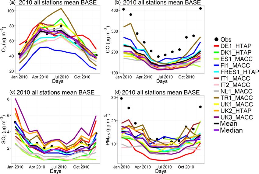
U. Im et al.: Assessment and economic valuation of air pollution impacts on human health                                     5969

et al. (2016), using the Atmospheric Chemistry and Climate        PM2.5 -related mortality. They found that the combined effect
Model Intercomparison Project (ACCMIP) model ensemble,            of climate change and emission reductions will reduce the
calculated that the global mortality burden of ozone is es-       premature mortality due to air pollution, in agreement with
timated to markedly increase from 382 000 deaths in 2000          the results from Schucht et al. (2015).
to between 1.09 and 2.36 million in 2100. They also calcu-           The US Environmental Protection Agency estimated that
lated that the global mortality burden of PM2.5 is estimated      in 2010 there were ∼ 160 000 premature deaths in the US due
to decrease from 1.70 million deaths in 2000 to between 0.95      to air pollution (US EPA, 2011). Fann et al. (2012) calculated
and 1.55 million deaths in 2100. Silva et al. (2013) esti-        130 000–350 000 premature deaths associated with O3 and
mated that in 2000, 470 000 premature respiratory deaths are      PM2.5 from the anthropogenic sources in the US for the year
associated globally and annually with anthropogenic ozone         2005. Caiazzo et al. (2013) estimated 200 000 cases of pre-
and 2.1 million deaths with anthropogenic PM2.5 -related car-     mature deaths in the US due to air pollution from combustion
diopulmonary diseases (93 %) and lung cancer (7 %). These         sources for the year 2005.
studies employed global chemistry–transport models with              The health impacts of air pollution and their economic
coarse spatial resolution (≥ 0.5◦ × 0.5◦ ); therefore, health     valuation are estimated based on observed and/or modeled
benefits from reducing local emissions were not able to be        air pollutant concentrations. Observations have spatial limi-
adequately captured. Higher resolutions are necessary to cal-     tations particularly when assessments are needed for large re-
culate more robust estimates of health benefits from local vs.    gions. The impacts of air pollution on health can be estimated
non-local sources (Fenech et al., 2017). In addition, these       using models, where the level of complexity can vary de-
studies calculated the number of premature deaths due to air      pending on the geographical scale (global, continental, coun-
pollution; however, none of them address morbidity such as        try or city), concentration input (observations, model calcu-
number of lung cancer or asthma cases, or restricted activity     lations, emissions) and the pollutants of interest that can vary
days. Finally, these studies did not include economic costs ei-   from only few (PM2.5 or O3 ) to a whole set of all regulated
ther. On the other hand, there are a number of regional studies   pollutants. The health impact models normally used may dif-
that calculate health impacts on finer spatial resolutions and    fer in the geographical coverage, spatial resolutions of the air
address morbidity. However, they are mostly based on sin-         pollution model applied, complexity of described processes,
gle air pollution models or do not evaluate the health benefits   the exposure–response functions (ERFs), population distri-
from local vs. non-local emissions. Therefore, a comprehen-       butions and the baseline indices (see Anenberg et al., 2015
sive study employing a multi-model ensemble of high spa-          for a review).
tial resolution and focusing on both mortality and morbidity         Air-pollution-related health impacts and associated costs
from local vs. non-local sources is lacking in the literature.    can be calculated using a chemistry–transport model (CTM)
   In Europe, recent results show that outdoor air pollution      or with standardized source–receptor relationships charac-
due to O3 , CO, SO2 and PM2.5 causes a total number of            terizing the dependence of ambient concentrations on emis-
570 000 premature deaths in the year 2011 (Brandt et al.,         sions (e.g., EcoSense model: ExternE, 2005; TM5-FASST:
2013a, b). The external (or indirect) costs to society re-        Van Dingenen et al., 2014). Source–receptor relationships
lated to health impacts from air pollution are tremendous.        have the advantage of reducing the computing time signifi-
OECD (2014) estimates that outdoor air pollution is costing       cantly and have therefore been extensively used in systems
its member countries USD 1.57 trillion in 2010. Among the         like GAINS (Amann et al., 2011). On the other hand, full
OECD member countries, the economic valuation of air pol-         CTM simulations have the advantage of better accounting for
lution in the US was calculated to be ∼ USD 500 billion, and      non-linear chemistry–transport processes in the atmosphere.
∼ USD 660 billion in Europe. In all of Europe, the total ex-         CTMs are useful tools to calculate the concentrations of
ternal costs have been estimated to approximately EUR 800         health-related pollutants taking into account non-linearities
billion in the year 2011 (Brandt et al., 2013a). These soci-      in the chemistry and the complex interactions between mete-
etal costs have great influence on the general level of wel-      orology and chemistry. However, the CTMs include different
fare and especially on the distribution of welfare both within    chemical and aerosol schemes that introduce differences in
the countries, as air pollution levels are vastly heterogeneous   the representation of the atmosphere as well as differences
both at regional and local scales, and between the countries,     in the emissions and boundary conditions they use (Im et al.,
as air pollution and the related health impacts are subject to    2015a, b). These different approaches are present also in the
long-range transport. Geels et al. (2015), using two regional     health impact estimates that use CTM results as the basis for
chemistry–transport models, estimated a premature mortality       their calculations. Multi-model (MM) ensembles can be use-
of 455 000 and 320 000 in the 28 member states of the Eu-         ful to the extent that allows us to take into consideration sev-
ropean Union (EU-28) for the year 2000, respectively, due         eral model results at the same time, define the relative weight
to O3 , CO, SO2 and PM2.5 . They also estimated that climate      of the various members in determining the mean behavior
change alone will lead to a small increase (15 %) in the to-      and produce also an uncertainty estimate based on the diver-
tal number of O3 -related acute premature deaths in Europe        sity of the results (Potempski et al., 2010; Riccio et al., 2012;
towards the 2080s and relatively small changes (< 5 %) for        Solazzo et al., 2013).

www.atmos-chem-phys.net/18/5967/2018/                                              Atmos. Chem. Phys., 18, 5967–5989, 2018
5970 U. Im et al.: Assessment and economic valuation of air pollution impacts on human health
The third phase of the Air Quality Modelling Evaluation
and the perturbation scenarios they performed.
Table 1. Key features (meteorological/chemistry–transport models, emissions, horizontal and vertical grids) of the regional models participating to the AQMEII3 health impact study
US3
UK3
UK2
UK1
TR1
NL1
IT2
IT1
FRES1
FI1
ES1
DK1
DE1
code
Group
International Initiative (AQMEII3) project brought together
14 European and North American modeling groups to sim-
ulate the air pollution levels over the two continental areas
WRF/CMAQ
WRF/CMAQ
WRF/CMAQ
WRF/CMAQ
WRF/CMAQ
LOTOS/EUROS
WRF/CAMx
WRF/CHEM
ECMWF/CHIMERE
ECMWF/SILAM
WRF/CHEM
WRF/DEHM
COSMO-CLM/CMAQ
Model
for the year 2010 (Galmarini et al., 2017). Within AQMEII3,
the simulated surface concentrations of health-related air pol-
lutants from each modeling group serve as input to the Eco-
nomic Valuation of Air Pollution (EVA) model (Brandt et al.,
2013a, b). The EVA model is used to calculate the impacts of
health-related pollutants on human health over the two con-
SMOKE
MACC
HTAP
MACC
MACC
MACC
MACC
MACC
HTAP
MACC
MACC
HTAP
HTAP
Emissions
tinents as well as the associated external costs. EVA model
has also been tested and validated for the first time outside
Europe. We adopt a MM ensemble approach, in which the
outputs of the modeling systems are statistically combined
12 km × 12 km
18 km × 18 km
30 km × 30 km
15 km × 15 km
30 km × 30 km
23 km × 23 km
23 km × 23 km
23 km × 23 km
50 km × 50 km
24 km × 24 km
0.50◦ × 0.25◦
0.25◦ × 0.25◦
0.25◦ × 0.25◦
assuming equal contribution from each model and used as in-
Horizontal
resolution
put for the EVA model. In addition, the human health impacts
(and the associated costs) of reducing anthropogenic emis-
sions, globally and regionally, have been calculated, allowing
to quantify the trans-boundary benefits of emission reduction
23 layers, 100 hPa
23 layers, 100 hPa
29 layers, 100 hPa
35 layers, 50 hPa
24 layers, 10 hPa
33 layers, 50 hPa
33 layers, 50 hPa
30 layers, 50 hPa
35 layers, 16 km
12 layers, 13 km
4 layers, 3.5 km
9 layers, 50 hPa
14 layers, 8 km
strategies. Finally, following the conclusions of Solazzo and
Galmarini (2015), the health impacts have been calculated
resolution
Vertical
using an optimal ensemble of models, determined by error
minimization. This approach can assess the health impacts
with reduced model bias, which we can then compare with
CB5-TUCL
CB5
CB5-TUCL
CB5-TUCL
CB5
CB4
CB5
RACM-ESRL
MELCHIOR2
CB4
RADM2
al. (2012)
Brandt et
CB5-TUCL
Gas phase
the classically derived estimates based on model averaging.
2 Material and methods
3 modes
3 modes
3 modes
3 modes
3 modes
VBS
2 modes,
3 modes
MADE/VBS
3 modes,
8 bins
VBS
1–5 bins,
MADE/SORGAM
3 modes,
2 modes
3 modes
model
Aerosol
2.1 AQMEII3
2.1.1 Participating models
In the framework of the AQMEII3 project, 14 groups par-
BASE
x
x
x
x
x
x
x
x
x
x
x
x
ticipated in simulating the air pollution levels in Europe and
North America for the year 2010. In the present study, we use GLO
results from the 13 groups that provided all health-related
x
x
x
x
x
x
x
x
x
x
species (Table 1). As seen in Table 1, six groups have op- Europe
NAM
erated the CMAQ model. The main differences among the
x
x
x
x
x
x
x
x
CMAQ runs reside in the number of vertical levels and hori-
zontal spacing (Table 1), and in the estimation of biogenic
EUR
x
x
x
x
x
x
emissions. UK1, DE1 and US3 calculated biogenic emis-
sions using the BEIS (Biogenic Emission Inventory System
BASE
version 3) model, while TR1, UK1 and UK2 calculated bio-
x
x
x
genic emissions through the Model of Emissions of Gases
North America
GLO
and Aerosols from Nature (MEGAN) (Guenther et al., 2012).
x
x
x
Moreover, DE1 does not include the dust module, while the
other CMAQ instances use the inline calculation (Appel et
EAS
x
x
x
al., 2013), and TR1 uses the dust calculation previously cal-
culated for AQMEII phase 2. Finally, all runs were carried
NAM
x
x
x
out using CMAQ version 5.0.2, except for TR1, which is
based on the 4.7.1 version. The gas-phase mechanisms and
the aerosol models used by each group are also presented in
Table 1. More details of the model system are provided in the
Supplement. The differences in the meteorological drivers
Atmos. Chem. Phys., 18, 5967–5989, 2018 www.atmos-chem-phys.net/18/5967/2018/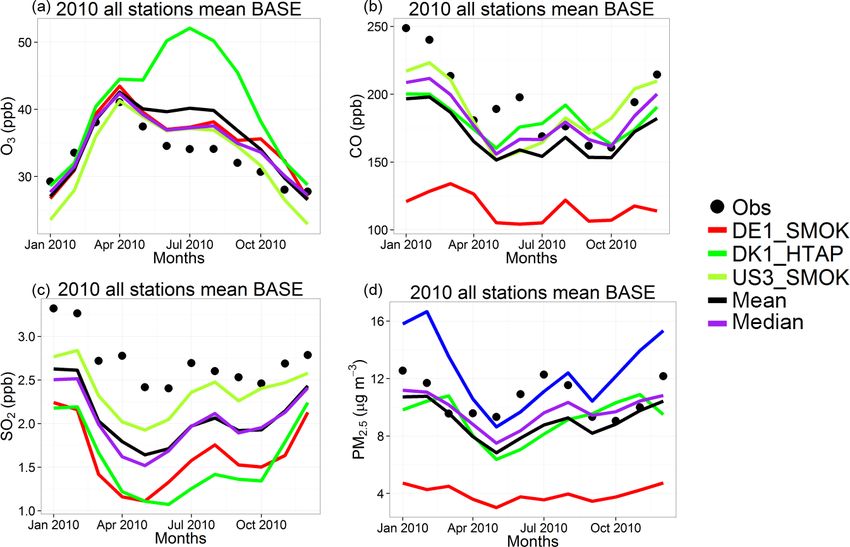
U. Im et al.: Assessment and economic valuation of air pollution impacts on human health                               5971

and aerosol modules can lead to substantial differences in     ing and Evaluation Programme (EMEP; http://www.emep.
modeled concentrations (Im et al., 2015b).                     int/) and the European Air Quality Database (AirBase; http:
                                                               //acm.eionet.europa.eu/databases/airbase/). In NA, observa-
2.1.2   Emission and boundary conditions                       tional data were obtained from the NAtChem (Canadian Na-
                                                               tional Atmospheric Chemistry) database and from the Anal-
The base case emission inventories that are used in AQMEII     ysis Facility operated by Environment Canada (http://www.
for Europe and North America are extensively described in      ec.gc.ca/natchem/).
Pouliot et al. (2015). For Europe, the 2009 inventory of the      The model evaluation has been conducted for 491 Euro-
Netherlands Organisation for Applied Scientific Research       pean and 626 North American stations for O3 , 541 European
Monitoring Atmospheric Composition and Climate (TNO-           stations and 37 North American stations for CO, 500 Euro-
MACC) anthropogenic emissions was used. In regions not         pean station and 277 North American stations for SO2 , and
covered by the emission inventory, such as north Africa,       568 European stations and 156 North American stations for
five modeling systems have complemented the standard in-       PM2.5 .
ventory with the HTAPv2.2 datasets (Janssens-Maenhout et
al., 2015). For the North American domain, the 2008 Na-        2.1.4    Emission perturbations
tional Emission Inventory was used as the basis for the 2010
emissions, providing the inputs and datasets for process-      In addition to the base case simulations in AQMEII3, a num-
ing with the SMOKE emissions processing system (Mason          ber of emission perturbation scenarios have been simulated
et al., 2007). For both continents, the regional-scale emis-   (Table 1). The perturbation scenarios feature a reduction of
sion inventories were embedded in the global-scale inventory   20 % in the global anthropogenic emissions (GLO) as well as
(Janssens-Maenhout et al., 2015) used by the global-scale      the HTAP2-defined regions of Europe (EUR), North Amer-
HTAP2 modeling community so as to guarantee coherence          ica (NAM) and east Asia (EAS), as explained in detail in
and harmonization of the information used by the regional-     Galmarini et al. (2017) and Im et al. (2018). To prepare these
scale modeling community. The annual totals for European       scenarios, both the regional models and the global C-IFS
and North American emissions in the HTAP inventory are         model that provides the boundary conditions to the partici-
the same as the MACC and SMOKE emissions. However,             pating regional models have been operated with the reduced
there are differences in the temporal distribution, chemical   emissions. The global perturbation scenario (GLO) reduces
speciation and the vertical distribution used in the models.   the global anthropogenic emissions by 20 %, introducing a
The C-IFS model (Flemming et al., 2015, 2017) provided         change in the boundary conditions as well as a 20 % decrease
chemical boundary conditions. The C-IFS model has been         in the anthropogenic emissions used by the regional models.
extensively evaluated in Flemming et al. (2015, 2017) and in   The North American perturbation scenario (NAM) reduces
particular for North America (Hogrefe et al., 2018; Huang et   the anthropogenic emissions in North America by 20 %, in-
al., 2017). Galmarini et al. (2017) provides more details on   troducing a change in the boundary conditions while anthro-
the setup of the AQMEII3 and HTAP2 projects.                   pogenic emissions remain unchanged for Europe, showing
                                                               the impact of long-range transport for North America, while
2.1.3   Model evaluation                                       the scenarios introduce a 20 % reduction of anthropogenic
                                                               emissions in the HTAP-defined North American region. The
The models’ performance in simulating the surface concen-      European perturbation scenario (EUR) reduces the anthro-
trations of the health-related pollutants were evaluated us-   pogenic emissions in the HTAP-defined European domain by
ing Pearson’s correlation (r), normalized mean bias (NMB),     20 %, introducing a change in the anthropogenic emissions
normalized mean gross error (NMGE) and root mean square        while boundary conditions remain unchanged in the regional
error (RMSE) to compare the modeled and observed hourly        models, showing the contribution from the domestic anthro-
pollutant concentrations over surface measurement stations     pogenic emissions only. Finally, the east Asian perturbation
in the simulation domains. The hourly modeled vs. observed     scenario (EAS) reduces the anthropogenic emissions in east
pairs are averaged and compared on a monthly basis. The        Asia by 20 %, introducing a change in the boundary con-
modeled hourly concentrations were first filtered based on     ditions while anthropogenic emissions remain unchanged in
observation availability before the averaging was performed.   the regional models, showing the impact of long-range trans-
The observational data used in this study are the same as      port from east Asia on the NA concentrations.
those in the dataset used in the second phase of AQMEII
(Im et al., 2015a, b). Surface observations are provided in    2.2     Health impact assessment
the ENSEMBLE system (http://ensemble.jrc.ec.europa.eu/)
that is hosted at the Joint Research Centre (JRC). Obser-      All modeling groups interpolate their model outputs on a
vational data were originally derived from the surface air     common 0.25◦ × 0.25◦ resolution AQMEII grid predefined
quality monitoring networks operating in EU and NA. In         for Europe (30◦ W–60◦ E, 25–70◦ N) and North America
EU, surface data were provided by the European Monitor-        (130–59.5◦ W, 23.5– 58.5◦ N). All the analyses performed in

www.atmos-chem-phys.net/18/5967/2018/                                           Atmos. Chem. Phys., 18, 5967–5989, 2018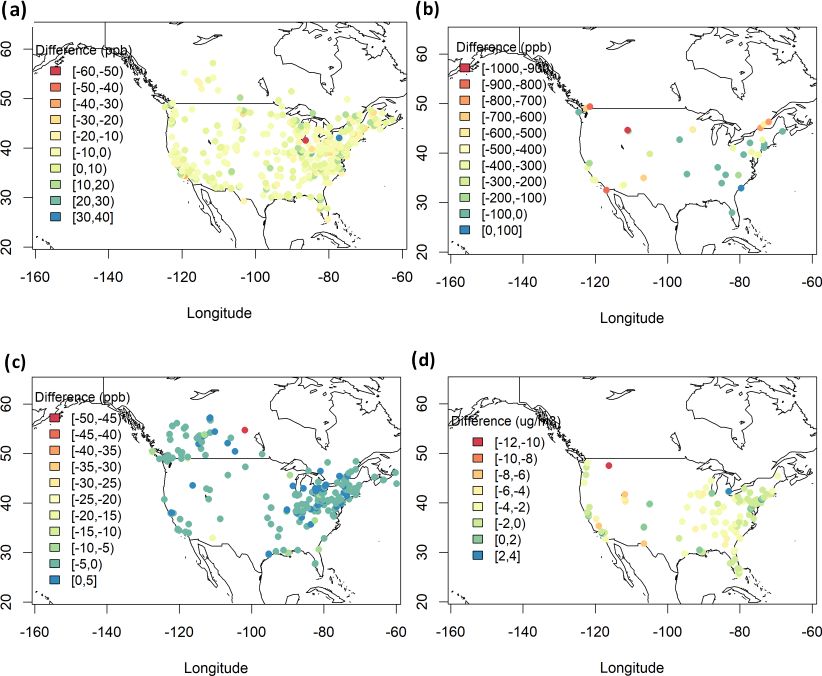
5972 U. Im et al.: Assessment and economic valuation of air pollution impacts on human health
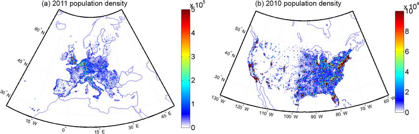
Figure 1. Population density (population per 0.25◦ × 0.25◦ grid box) over (a) the United States and (b) Europe.
the present study use the pollutant concentrations on these fi- sidering that for the main pollutants (O3 and PM2.5 ) the net-
nal grids. Health impacts are first calculated for each individ- work of measurements is quite dense around densely popu-
ual model, and then the ensemble mean, median and standard lated areas (where the inputs of the MM ensemble are used
deviation are calculated for each health impact. In order to be for assessing the impact of air pollutants on the health of the
able to estimate an uncertainty in the health impact calcula- population), errors due to inaccurate model selection in re-
tions, none of the models were removed from the ensemble. mote regions might be regarded as negligible (Solazzo and
Along with the individual health impact estimates from Galmarini, 2015). It should be noted that the selection of the
each model, a multi-model mean dataset (MMm , in which optimal combinations of models is affected by the model’s
all the modeling systems are averaged assuming equally bias that might stem from processes that are common to all
weighted contributions) has been created for each grid cell members of the ensemble (e.g., emissions). Therefore, such a
and time step, hence creating a new model set of results common bias does not cancel out when combining the mod-
that have the same spatial and temporal resolution of the els, possibly creating a biased ensemble. Current work is be-
ensemble-contributing members. In addition to this simple ing devoted to identify the optimal combinations of models
MMm , an optimal MM ensemble (MMopt ) has been gen- from which the offsetting bias is removed (Solazzo et al.,
erated. MMopt is created following the criteria extensively 2018).
discussed and tested in the previous phases of the AQMEII
activity (Riccio et al., 2012; Kioutsioukis et al., 2016; So- 2.2.1 EVA system
lazzo and Galmarini, 2016), where it was shown that there
are several ways to combine the ensemble members to ob- The EVA system (Brandt et al., 2013a, b) is based on the
tain a superior model, mostly depending on the feature we impact-pathway chain (e.g., Friedrich and Bickel, 2001),
wish to promote (or penalize). For instance, generating an consisting of the emissions, transport and chemical trans-
optimal ensemble that maximizes the accuracy would require formation of air pollutants, population exposure, health im-
a minimization of the mean error or of the bias, while maxi- pacts and the associated external costs. The EVA system re-
mizing the associativity (variability) would require maximiz- quires hourly gridded concentration input from a regional-
ing the correlation coefficient (standard deviation). In this scale CTM as well as gridded population data, ERFs for
study, the subset of models whose means minimize the mean health impacts and economic valuations of the impacts from
squared error (MSE) is selected as optimal (MMopt ). MMm air pollution. A detailed description of the integrated EVA
and MMopt have therefore the same spatial resolution with model system along with the ERFs and the economic valua-
the individual models. The MSE is chosen for continuity tions used are given in Brandt et al. (2013a).
with previous AQMEII-related works. The MSE is chosen The gridded population density data over Europe and the
in light of its property of being composed by bias, variance US used in this study are presented in Fig. 1. The population
and covariance types of error, thus lumping together mea- data over Europe are provided on a 1 km spatial resolution
sures of accuracy (bias), variability (variance) and associa- from Eurostat for the year 2011 (http://www.efgs.info). The
tivity (covariance) (Solazzo and Galmarini, 2016). The min- US population data have been provided by the US Census
imum MSE has been calculated at the monitoring stations, Bureau for the year 2010. The total populations used in this
where observational data are available, and then extended to study are roughly 532 and 307 million in Europe and the US,
the entire continental areas. This approximation might affect respectively. As the health outcomes are age dependent, the
remote regions away from the measurements. However, con- total population data have been broken down to a set of age
intervals as follows: babies (under 9 months); children (un-
Atmos. Chem. Phys., 18, 5967–5989, 2018 www.atmos-chem-phys.net/18/5967/2018/U. Im et al.: Assessment and economic valuation of air pollution impacts on human health 5973
Table 2. Exposure–response functions, the concentrations metrics and economic valuations used in the EVA model. “EU27” are the member
states of the European Union between 2007 and 2013.
Health effects (compounds) Exposure–response coefficient Valuation, EUR2013
(α) (EU27 & NA)
Morbidity
Chronic bronchitis1 , CB (PM) 8.2E-5 cases µg−1 m−3 (adults) 38 578 per case
Restricted activity days2 , RAD (PM) = 8.4 E-4 days µg−1 m−3 (adults) 98 per day
−3.46E-5 days µg−1 m−3 (adults)
−2.47E-4 days µg−1 m−3 (adults > 65)
−8.42E-5 days µg−1 m−3 (adults)
Congestive heart failure3 , CHF (PM) 3.09E-5 cases µg−1 m−3 10 998 per case
Congestive heart failure3 , CHF (CO) 5.64E-7 cases µg−1 m−3
Lung cancer4 , LC (PM) 1.26E-5 cases µg−1 m−3 16 022 per case
Hospital admissions
Respiratory5 , RHA (PM) 3.46E-6 cases µg−1 m−3 5315 per case
Respiratory5 , RHA (SO2 ) 2.04E-6 cases µg−1 m−3
Cerebrovascular6 , CHA (PM) 8.42E-6 cases µg−1 m−3 6734 per case
Asthma children (7.6 % < 16 years)
Bronchodilator use7 , BUC (PM) 1.29E-1 cases µg−1 m−3 16 per case
Cough8 , COUC (PM) 4.46E-1 days µg−1 m−3 30 per day
Lower respiratory symptoms7 , LRSA (PM) 1.72E-1 days µg−1 m−3 9 per day
Asthma adults (5.9 % > 15 years)
Bronchodilator use9 , BUA (PM) 2.72E-1 cases µg−1 m−3 16 per case
Cough9 , COUA (PM) 2.8E-1 days µg−1 m−3 30 per day
Lower respiratory symptoms9 , LRSA (PM) 1.01E-1 days µg−1 m−3 9 per day
Mortality
Acute mortality10,11 (SO2 ) 7.85E-6 cases µg−1 m−3 1 532 099 per case
Acute mortality10,11 (O3 ) 3.27E-6 × SOMO35 cases µg−1 m−3
Chronic mortality4,12, , YOLL (PM) 1.138E-3 YOLL µg−1 m−3 (> 30 years) 57 510 per YOLL
Infant mortality13 , IM (PM) 6.68E-6 cases µg−1 m−3 (> 9 months) 2 298 148 per case
1 Abbey et al. (1995). 2 Ostro (1987). 3 Schwartz and Morris (1995). 4 Pope et al. (2002). 5 Dab et al. (1996). 6 Wordley et al. (1997). 7 Roemer
et al. (1993). 8 Pope and Dockerey (1992). 9 Dusseldorp et al. (1995). 10 Anderson et al. (1996). 11 Touloumi et al. (1996). 12 Pope et al. (1995).
13 Woodruff et al. (1997).
der 15); and adults above 15, above 30 and above 65. The impacts are calculated using an ERF of the following form:
fractions of population in these intervals for Europe are de-
rived from the Eurostat 2000 database, where the number of R = α × δc × P ,
persons of each age at each grid cell was aggregated into the
where R is the response (in cases, days or episodes), c de-
above clusters (Brandt et al., 2011), while for the US they
notes the pollutant concentration, P denotes the affected
are derived from the US Census Bureau for the year 2010 at
share of the population, and α is an empirically determined
5-year intervals.
constant for the particular health outcome. EVA uses ERFs
The EVA system can be used to assess the number of vari-
that are modeled as a linear function, which is a reasonable
ous health outcomes including different morbidity outcomes
approximation as showed in several studies (e.g., Pope, 2000;
as well as short-term (acute) and long-term (chronic) mortal-
the joint World Health Organization/UNECE Task Force on
ity, related to exposure of O3 , CO and SO2 (short term) and
Health; EU, 2004; Watkiss et al., 2005). Many epidemi-
PM2.5 (long term). Furthermore, impact on infant mortality
ological studies have analyzed the concentration–response
in response to exposure of PM2.5 is calculated. The health
relationship between ambient PM and mortality using var-
ious statistical models. In general, the shapes of the esti-
www.atmos-chem-phys.net/18/5967/2018/ Atmos. Chem. Phys., 18, 5967–5989, 20185974 U. Im et al.: Assessment and economic valuation of air pollution impacts on human health mated curves did not differ significantly from linear. How- annual PM2.5 increase of 10 µg m−3 (Andersen et al., 2008). ever, some studies showed non-linear relationships, being EVA uses a counterfactual PM2.5 concentration of 0 µg m−3 steeper at lower than at higher concentrations (e.g., Samoli et following the EEA methodology, meaning that the impacts al., 2005). Therefore, linear relationships may lead to over- have been estimated for the full range of modeled concen- estimated health impacts over highly polluted concentration trations from 0 µg m−3 upwards. Applying a low counterfac- metrics used in each ERF shown in Table 2. The sensitivity of tual concentration can underestimate health impacts at low EVA to the different pollutant concentrations is further eval- concentrations if the relationship is linear or close to lin- uated in the the Supplement and depicted in Fig. S1. EVA ear (Anenberg et al., 2015). However, it is important to note calculates and uses the annual mean concentrations of CO, that uncertainty in the health impact results may increase at SO2 and PM2.5 , while for O3 , it uses the SOMO35 metric low concentrations due to sparse epidemiological data. As- that is defined as the yearly sum of the daily maximum of suming linearity at very low concentrations may distort the 8 h running average over 35 ppb, following WHO (2013) and true health impacts of air pollution in relatively clean atmo- EEA (2017). spheres (Anenberg et al., 2016). The morbidity outcomes include chronic bronchitis, re- It has been shown that O3 concentrations above the stricted activity days, congestive heart failure, lung cancer, level of 35 ppb involve an acute mortality increase, presum- respiratory and cerebrovascular hospital admissions, asthma ably for weaker and elderly individuals. EVA applies the in children (< 15 years) and adults (> 15 years), which ERFs selected in CAFE for post-natal deaths (age group 1– includes bronchodilator use, cough and lower respiratory 12 months) and acute deaths related to O3 (Hurley et al., symptoms. The exposure–response functions are broadly in 2005). WHO (2013a) also recommends the use of the daily line with estimates derived with detailed analysis in EU- maximum of 8 h mean O3 concentrations for the calculation funded research (Rabl et al., 2014; EEA, 2013). To figure of the acute mortality due to O3 . There are also studies show- out the total number of premature deaths from the years of ing that SO2 is associated with acute mortality, and EVA life lost due to PM2.5 , they have been converted into lost adopts the ERF identified in the APHENA study – Air Pollu- lives according to a “lifetable” method (explained in de- tion and Health: A European Approach (Katsouyanni et al., tail in Andersen, 2017) but using the factor of 10.6, as re- 1997). ported by Watkiss et al. (2005). To these deaths are added Chronic exposure to PM2.5 is also associated with mor- the acute deaths due to O3 and SO2 . The ERFs used, along bidity, such as lung cancer. EVA employs the specific ERF with their references, in both continents as well as the eco- (RR of 1.08 per 10 µg m−3 PM2.5 increase) for lung cancer nomic valuations for each health outcome in Europe and the indicated in Pope et al. (2002). Bronchitis has been shown US, respectively, are presented in Table 2. Baseline incidence to increase with chronic exposure to PM2.5 and we apply rates are not assumed to be dissimilar, which is a coarse ap- an ERF (RR of 1.007) for new cases of bronchitis based on proach for morbidity. The baseline rates are from Statistics the AHSMOG study (involving non-smoking Seventh-Day Denmark (http://www.statistikbanken.dk/statbank5a/default. Adventists; Abbey et al., 1999), which is the same epidemi- asp?w=1280, last access: 25 April 2018) and lifetables are ological study as in CAFE (Abbey et al., 1995; Hurley et based on Denmark, which is close to the US and Eurozone al., 2005). The ExternE crude incidence rate was chosen as a average (Andersen, 2017). For a description of the morbid- background rate (ExternE, 1999), which is in agreement with ity ERFs, see Andersen et al. (2004, 2008). The economic a Norwegian study, rather than the pan-European estimates valuations are provided by Brandt et al. (2013a); see also used in CAFE (Eagan et al., 2002). Restricted activity days EEA (2013). (RADs) comprise two types of responses to exposure: so- ERFs for all-cause chronic mortality due to PM2.5 were called minor restricted activity days as well as work-loss days based on the findings of Pope et al. (2002), which is the (Ostro, 1987). This distinction enables accounting for the dif- most extensive study available, following conclusions from ferent costs associated with days of reduced well-being and the scientific review of the Clean Air For Europe (CAFE) actual sick days. It is assumed that 40 % of RADs are work- program (Hurley et al., 2005; Krupnick et al., 2005). The loss days based on Ostro (1987). The background rate and results from Pope et al. (2002) are further supported by incidence are derived from ExternE (1999). Hospital admis- Krewski et al. (2009) and more recently by the latest sions are deducted to avoid any double counting. Hospital ad- HRAPIE project report (WHO, 2013a). Therefore, as recom- missions and health effects for asthmatics (here correspond- mended by WHO (2013a), EVA uses the ERFs based on the ing to the responses of bronchodilator use, cough and lower meta-analysis of 13 cohort studies as described in Hoek et respiratory symptoms) are also based on ExternE (1999). al. (2013). In EVA, the number of lost life years for a Dan- Table 2 lists the specific valuation estimates applied in the ish population cohort with normal age distribution, when ap- modeling of the economic valuation of mortality and mor- plying the ERF of Pope et al. (2002) for all-cause mortal- bidity effects. A principal value of EUR 1.5 million was ap- ity (relative risk, RR of 1.062 (1.040–1.083) on a 95 % con- plied for preventing an acute death, following expert panel fidence interval), and the latency period indicated, sums to advice (EC, 2001). For the valuation of a life year, the results 1138 years of life lost (YOLL) per 100 000 individuals for an from a survey relating specifically to air pollution risk reduc- Atmos. Chem. Phys., 18, 5967–5989, 2018 www.atmos-chem-phys.net/18/5967/2018/
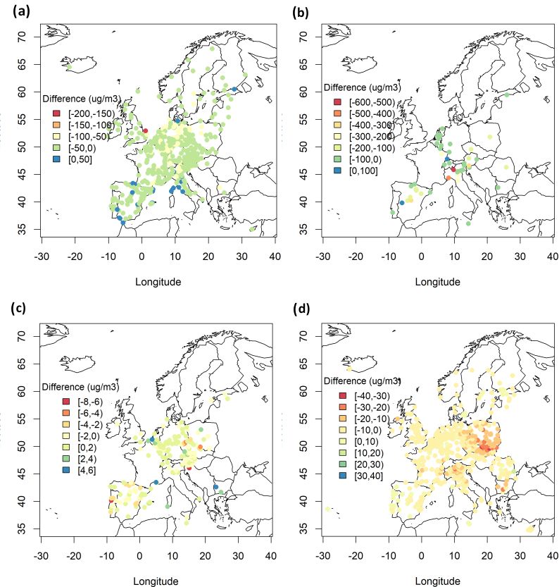
U. Im et al.: Assessment and economic valuation of air pollution impacts on human health                                     5975

tions were applied (Alberini et al., 2006), implying a value        such benefit transfer. The unit values have been indexed to
of EUR 57 500 per year of life lost (YOLL). With the more           2013 prices as indicated in Table 2.
conservative metric of estimating lost life years, rather than
“full” statistical lives, there is no adjustment for age. This is
due to the fact that government agencies in Europe, including       3     Results
the European Commission, apply a methodology for costs of
air pollution that is based on accounting for lost life years,      3.1    Model evaluation
rather than for entire statistical lives as is customary in USA.
While the average traffic victim, for instance, is middle-aged      Observed and simulated hourly surface O3 , CO, SO2 and
and likely to lose about 35–40 years of life expectancy, pollu-     daily PM2.5 , which are species used in the EVA model to
tion victims are believed to suffer significantly smaller losses    calculate the health impacts, over Europe and North America
of years (EAHEAP, 1999; Friedrich and Bickel, 2001). To             for the entire 2010 were compared in order to evaluate each
avoid overstating the benefits of air pollution control, these      model’s performance. The statistical parameters to evaluate
are treated as proportional to the number of life years lost.       the models and their equations are provided in the Supple-
Most of the excess mortality is due to chronic exposure to          ment. For a more thorough evaluation of models and species,
air pollution over many years, and the life year metric is          see Solazzo et al. (2017). The results of this comparison are
based on the number of lost life years in a statistical cohort.     presented in Table S1 for EU and NA, along with the multi-
Following the guidelines of the Organisation for Economic           model mean and median values. The monthly time series
Co-operation and Development (OECD, 2006), the predicted            plots of observed and simulated health-related pollutants are
acute deaths, mainly from O3 , are valuated here with the ad-       also presented in Figs. 2 and 3. The monthly means are calcu-
justed value for preventing a fatality (VSL, value of a statisti-   lated using the hourly pairs of observed and modeled concen-
cal life). The lifetables are obtained from European data and       trations at each station. The results show that, over Europe,
are applied to the US as the average life expectancy in the         the temporal variability of all gaseous pollutants is well cap-
US is similar to that in Europe and close to the OECD aver-         tured by all models with correlation coefficients (r) higher
age (OECD, 2016). The willingness to pay for reductions in          than 0.70 in general. The NMBs in simulated O3 levels are
risk obviously differs across income levels. However, in the        generally below 10 % with few exceptions up to −35 %. CO
case of air pollution costs, adjustment according to per capita     levels are underestimated by up to 45 %, while the major-
income differences among different states is not regarded as        ity of the models underestimated SO2 levels by up to 68 %,
appropriate, because long-range transport implies that emis-        while some models overestimated SO2 by up to 49 %. PM2.5
sions from one state will affect numerous other states and          levels are underestimated by 19 to 63 %. Over Europe, the
their citizens. The valuations are thus adjusted with regional      median of the ensemble performs better than the mean in
purchasing power parities (PPPs) of EU27 and USA.                   terms of model bias (NMB) for O3 (by 52 %), while for CO,
   Cost–benefit analysis in the US related to air pollution pro-    SO2 and PM2.5 , the mean performs slightly better than the
ceeds from a standard approach, where abatement measures            median (Table S1).
preventing premature mortality are considered according to             We have further evaluated the models’ performance in
the number of statistical fatalities avoided, which are appre-      simulating the annual mean pollutant levels over individual
ciated according to the VSL (presently USD 7.4 million). In         measurements stations and plotted the geographical distribu-
contrast, and following recommendations from the UK work-           tion of the bias. Figure 4 presents the multi-model mean geo-
ing group on Economic Appraisal of the Health Effects of            graphical distribution of bias from daily max 8 h (DM8H) av-
Air Pollution (EAHEAP, 1999), focus in EU has been on the           erage O3 , CO, SO2 and PM2.5 over Europe, while Figs. S2–
possible changes in average life expectancy resulting from air      S5 show annual mean bias for O3 , CO, SO2 and PM2.5 for
pollution. In EU, the specific number of life years lost as a re-   each model, respectively. DM8H O3 levels over Europe are
sult of changes in air pollution exposures is estimated based       generally underestimated by up to 50 µg m−3 , with few over-
on lifetable methodology and monetized with value-of-life-          estimations up to 50 µg m−3 over southern Europe (Fig. 4a).
year (VOLY) unit estimates (Holland et al., 1999; Leksell           The geographical pattern of annual mean O3 bias is similar
and Rabl, 2001). The theoretical basis is a lifetime consump-       among the models with slight differences (±10 µg m−3 ) in
tion model according to which the preferences for risk re-          the bias (Fig. S2). CO levels are underestimated over all sta-
duction will reflect expected utility of consumption for re-        tions by up to 600 µg m−3 except for few stations where CO
maining life years (Hammitt, 2007; OECD, 2006, p. 204).             levels are overestimated by up to 100 µg m−3 (Fig. 4b). All
The much lower VSL values customary in Europe (presently            models underestimated CO levels over the majority of the
EUR 2.2 million) add decisively to the differences, as VOLY         stations (Fig. S3). SO2 levels are slightly overestimated over
is deducted from this value. By using a common valuation            central and southern Europe (Fig. 4c). There are also under-
framework according to the EU approach, we allow for direct         estimations over few stations with no specific geographical
comparisons of the monetary results. It follows from OECD           pattern. Similar to CO, all models underestimated SO2 lev-
recommendations (2012) to correct with PPP when doing               els over the majority of the stations (Fig. S4). Finally, PM2.5

www.atmos-chem-phys.net/18/5967/2018/                                                Atmos. Chem. Phys., 18, 5967–5989, 2018
5976                            U. Im et al.: Assessment and economic valuation of air pollution impacts on human health

Figure 2. Observed and simulated (base case) monthly (a) O3 , (b) CO, (c) SO2 and (d) PM2.5 concentrations over Europe.

Figure 3. Observed and simulated (base case) monthly (a) O3 , (b) CO, (c) SO2 and (d) PM2.5 concentrations over the US.

levels are underestimated by up to 10 µg m−3 over most of             DE1 model, having a large underestimation of 63 % (Ta-
Europe (Fig. 4d), with larger underestimations over eastern           ble S1). As DE1 and US3 use the same SMOKE emissions
Europe up to 30 µg m−3 .                                              and CTM, the large difference in PM2.5 concentrations can
   Over North America, the hourly O3 variation is well cap-           be partly due to the differences in horizontal and vertical
tured by all models (Table S1), with DK1 having slightly              resolutions in the model setups, as can also be seen in the
lower r coefficient compared to the other models and largest          differences in the CO concentrations. There are also dif-
NMB (Fig. 3a). The hourly variations of CO and SO2 lev-               ferences in the aerosol modules and components that each
els are simulated with relatively lower r values (Fig. 3b, c),        model simulates. For example, DE1 uses an older version
with SO2 levels having the highest underestimations. The              of the secondary organic aerosol (SOA) module, producing
PM2.5 levels are underestimated by ∼ 15 % except for the              ∼ 3 µg m−3 less SOA, which can explain ∼ 20 % of the bias

Atmos. Chem. Phys., 18, 5967–5989, 2018                                                 www.atmos-chem-phys.net/18/5967/2018/
U. Im et al.: Assessment and economic valuation of air pollution impacts on human health                                       5977

Figure 4. Spatial distribution of annual MM mean bias (µg m−3 ) for (a) DM8H O3 , (b) CO, (c) SO2 and (d) PM2.5 over Europe.

over North America. Over the North American domain, the              ∼ 100 ppb over the majority of the stations, especially over
median outscores the mean for O3 (by 35 %), CO (by 52 %)             the eastern US, while there are much larger underestimations
and PM2.5 (by 29 %), while for SO2 , the median produces             over the western US by up to 1000 ppb (Fig. 5b). SO2 levels
26 % higher NMB compared to the mean. The DK1 model                  are underestimated by up to 5 ppb over the majority of the
simulates a much higher bias for O3 and SO2 compared to              stations in the US, with few overestimations of up to 5 ppb
other models in the North American domain, while DE1 has             (Fig. 5c). DE1 and DK1 have a very similar spatial distri-
the largest bias for CO and PM2.5 .                                  bution of bias, while US3 has slightly more overestimations
   DM8H O3 levels are generally underestimated by the MM             (Fig. S8). Finally, PM2.5 levels are underestimated over ma-
mean over the US by up to 20 ppb, while over the eastern             jority of the stations by up to 6 µg m−3 , with few overestima-
and central US there are also overestimations by up to 10 ppb        tions by 2–4 µg m−3 (Fig. 5d). DE1 has the largest underes-
(Fig. 5a). As seen in Fig. S6, all three models have very simi-      timations compared to DK1 and US3 (Fig. S9).
lar performance over the US, with DK1 simulating a slightly             Table S1 shows that the ensemble median performs
lower underestimation and a higher overestimation compared           slightly better than the ensemble mean for all pollutants over
to DE1 and US3. DE1 and DK1 have very similar spatial                both continents in terms of the bias and error, while the dif-
pattern in terms of CO bias, in particular over the eastern          ference in r is rather small. Over the European stations, the
coast of the US (Fig. S7). CO levels are underestimated by           median has improved results over the mean by up to 14 % for

www.atmos-chem-phys.net/18/5967/2018/                                                  Atmos. Chem. Phys., 18, 5967–5989, 2018
5978                            U. Im et al.: Assessment and economic valuation of air pollution impacts on human health

Figure 5. Spatial distribution of annual MM mean bias (ppb for gases and µg m−3 for PM2.5 ) for (a) DM8H O3 , (b) CO, (c) SO2 and
(d) PM2.5 over North America.

r and up to 9 % for the RMSE. The improvements in r over           ber of premature deaths due to air pollution is calculated to
the US are much smaller compared to Europe (up to ∼ 4 %),          be 230 000 to 570 000 (mean of all individual models, MMmi ,
while the RMSE is improved by up to 27 %, except for SO2           414 000 ± 100 000). The health impacts calculated as the me-
where the median has 14 % higher RMSE than the mean.               dian of individual models differ slightly (∼ ±1 %) from those
                                                                   calculated as the mean of individual models (Table S2) due
3.2    Health outcomes and their economic valuation in             to the slight differences in the model bias (NMB) and error
       Europe                                                      (NMGE and RMSE) between the mean and the median per-
                                                                   formance statistics of the models.
The different health outcomes calculated by each model in             In addition to averaging the health estimates from individ-
Europe as well as their multi-model mean and median are            ual models (MMmi ), we have also produced a multi-model
presented in Table S2. Table 3 presents the mean of the indi-      mean concentration data (MMm ) by taking the average of
vidual model estimates as MMmi . Standard deviations cal-          concentrations of each species calculated by all models at
culated from the individual model estimates are presented          each grid cell and hour, and feeding it to the EVA model.
along with the MMmi in the text. The health impact esti-           We have calculated the number of premature death cases in
mates vary significantly between different models. The dif-        Europe (Table 3) using MMm . The difference in the health
ferent estimates obtained are found to vary up to a factor of 3.   impacts calculated using MMm data from the mean of all in-
Among the different health outcomes, the individual mod-           dividual model (MMmi ) estimates is smaller than 1 %. The
els simulated the number of congestive heart failure (CHF)         number of premature death cases in Europe as calculated
cases to be between 19 000 and 41 000 (mean of all indi-           as the average of all models in the multi-model ensem-
vidual models, MMmi , 31 000 ± 6500). The number of lung           ble, MMmi , due to exposure to O3 is 12 000 ± 6500, while
cancer cases due to air pollution is calculated to be between      the cases due to exposure to PM2.5 are calculated to be
30 000 and 78 000 (mean of all individual models, MMmi ,           390 000 ± 100 000 (180 000–550 000). The O3 -related mor-
55 000 ± 14 000). Finally, the total (acute and chronic) num-

Atmos. Chem. Phys., 18, 5967–5989, 2018                                             www.atmos-chem-phys.net/18/5967/2018/
U. Im et al.: Assessment and economic valuation of air pollution impacts on human health 5979
Table 3. Health impacts calculated by the mean of individual model estimates (denoted as MMmi ) and the standard deviation, multi-model
mean ensemble without error reduction (MMm ) and the optimal ensemble (MMopt ) in Europe and the US. See Table 2 for the definitions
of health impacts. PD stands for premature deaths. All health impacts are in units of number of cases multiplied by 1000, except for infant
mortality (IM), which reports directly the number of cases.
EU NA
MMmi MMm MMopt MMmi MMm MMopt
CB 360 ± 89 360 468 142 ± 74 142 125
RAD 368 266 ± 90 670 368 245 478 073 145 337 ± 75 250 145 337 127 921
RHA 23 ± 5 23 28 10 ± 4 8 7
CHA 46 ± 11 46 60 19 ± 10 19 16
CHF 31 ± 6 31 38 13 ± 6 9 8
LC 55 ± 14 55 72 22 ± 11 22 19
BDUC 10 766 ± 2650 10 766 13 976 4566 ± 2383 4566 4019
BDUA 70 492 ± 17 400 70 489 91 511 27 819 ± 14 400 27 819 24 485
COUC 37 198 ± 9160 37 196 48 289 15 776 ± 8230 15 776 13 886
COUA 72 566 ± 17 900 72 562 94 203 28 637 ± 14 830 28 637 25 206
LRSC 14 355 ± 3530 14 354 18 635 6088 ± 3180 6088 5359
LRSA 26 175 ± 6400 26 174 33 980 10 330 ± 5350 10 330 9092
AYOLL 26 ± 13 23 20 25 ± 7 9 9
YOLL 4111 ± 1010 4111 5337 1481 ± 762 1481 1304
PD 414 ± 98 410 524 165 ± 76 149 133
IM 403 ± 99 403 524 143 ± 75 143.3667 126.1
tality well agrees with Liang et al. (2018), who used the Among all models, the DE1 model calculated the lowest
multi-model mean of the HTAP2 global model ensemble, health impacts for most health outcomes, which can be at-
which calculated an O3 -related mortality of 12 800 (600– tributed to the largest underestimation of PM2.5 levels (NMB
28 100). The multi-model mean (MMmi ) PM2.5 -related mor- of −63 %; Table S2) due to lower spatial resolution of the
tality in the present study is much higher than that in the model that dilutes the pollution in the urban areas, where
HTAP2 study: 195 500 (4400–454 800). The results also most of the population lives. The number of premature deaths
agree with the most recent EEA findings (EEA, 2015), which calculated by this study is in agreement with previous studies
calculated a total of 419 000 premature deaths due to O3 and for Europe using the EVA system (Brandt et al., 2013a; Geels
PM2.5 in the EU28 countries. There is also agreement with et al., 2015). Recently, EEA (2015) estimated that air pollu-
Geels et al. (2015), who calculated 388 000 premature death tion is responsible for more than 430 000 premature deaths in
cases in Europe for the year 2000. This difference can be at- Europe, which is in good agreement with the present study.
tributed to the number of mortality cases as calculated by the Figure 6a presents the geographical distribution of the
individual models, where the HTAP2 ensemble calculates a number of premature deaths in Europe in 2010. The figure
much lower minimum while the higher ends from the two shows that the number of cases is strongly correlated with the
ensembles agree well. population density (Fig. 1a), with the largest numbers seen in
The differences between the health outcomes calculated the Benelux and Po Valley regions that are characterized as
by the HTAP2 and AQMEII ensembles arise firstly from the the pollution hot spots in Europe as well as in megacities
differences in the concentration fields due to the differences such as London, Paris, Berlin and Athens.
in models, in particular spatial resolutions as well as the gas The economic valuation of the air-pollution-associated
and aerosol treatments in different models, but also the dif- health impacts calculated by the different models, along with
ferences in calculating the health impacts from these concen- their mean and median, is presented in Table 4. A total
tration fields. EVA calculates the acute premature deaths due cost of EUR 196 billion to 451 billion (MM mean cost of
to O3 by using the SOMO35 metric. On the other hand, in EUR 300 ± 70 billion) was estimated over Europe (EU28).
HTAP2, O3 -related premature deaths are calculated by us- Results show that 5 % (1–11 %) of the total costs are due to
ing the 6-month seasonal average of daily 1 h maximum O3 exposure to O3 , while 89 % (80–96 %) are due to exposure to
concentrations. Both groups use the annual mean PM2.5 to PM2.5 . Brandt et al. (2013a) calculated a total external cost
calculate the PM2.5 -related premature deaths. In addition to of EUR 678 billion for the year 2011 for Europe, larger than
O3 and PM2.5 , EVA also takes into account the health im- the estimates of this study, which can be explained by the dif-
pacts from CO and SO2 , which are missing in the HTAP2 ferences in the simulation year and the emissions used in the
calculations.
www.atmos-chem-phys.net/18/5967/2018/ Atmos. Chem. Phys., 18, 5967–5989, 2018You can also read