Modelling thermomechanical ice deformation using an implicit pseudo-transient method (FastICE v1.0) based on graphical processing units (GPUs) ...
←
→
Page content transcription
If your browser does not render page correctly, please read the page content below
Geosci. Model Dev., 13, 955–976, 2020
https://doi.org/10.5194/gmd-13-955-2020
© Author(s) 2020. This work is distributed under
the Creative Commons Attribution 4.0 License.

Modelling thermomechanical ice deformation using an implicit
pseudo-transient method (FastICE v1.0) based on graphical
processing units (GPUs)
Ludovic Räss1,a,b , Aleksandar Licul2,3 , Frédéric Herman2,3 , Yury Y. Podladchikov3,4 , and Jenny Suckale1
1 Stanford  University, Geophysics Department, 397 Panama Mall, Stanford, CA 94305, USA
2 Institute of Earth Surface Dynamics, University of Lausanne, 1015 Lausanne, Switzerland
3 Swiss Geocomputing Centre, University of Lausanne, 1015 Lausanne, Switzerland
4 Institute of Earth Sciences, University of Lausanne, 1015 Lausanne, Switzerland
a now at: Laboratory of Hydraulics, Hydrology and Glaciology (VAW), ETH Zurich, Zurich, Switzerland
b now at: Swiss Federal Institute for Forest, Snow and Landscape Research (WSL), Birmensdorf, Switzerland

Correspondence: Ludovic Räss (ludovic.rass@gmail.com)

Received: 3 September 2019 – Discussion started: 9 September 2019
Revised: 6 December 2019 – Accepted: 5 February 2020 – Published: 6 March 2020

Abstract. Ice sheets lose the majority of their mass through      lel version of FastICE to run on GPU-accelerated distributed
outlet glaciers or ice streams, corridors of fast ice moving      memory machines, reaching a parallel efficiency of 99 %. We
multiple orders of magnitude more rapidly than the surround-      show that our model is particularly useful for improving our
ing ice. The future stability of these corridors of fast-moving   process-based understanding of flow localisation in the com-
ice depends sensitively on the behaviour of their boundaries,     plex transition zones bounding rapidly moving ice.
namely shear margins, grounding zones and the basal sliding
interface, where the stress field is complex and fundamen-
tally three-dimensional. These boundaries are prone to ther-
momechanical localisation, which can be captured numeri-          1   Introduction
cally only with high temporal and spatial resolution. Thus,
better understanding the coupled physical processes that gov-     The fourth IPCC report (Solomon et al., 2007) concludes that
ern the response of these boundaries to climate change ne-        existing ice-sheet flow models do not accurately describe po-
cessitates a non-linear, full Stokes model that affords high      lar ice-sheet discharge (e.g. Gagliardini et al., 2013; Pattyn
resolution and scales well in three dimensions. This pa-          et al., 2008) owing to their inability to simultaneously model
per’s goal is to contribute to the growing toolbox for mod-       slow and fast ice motion (Gagliardini et al., 2013; Bueler and
elling thermomechanical deformation in ice by leveraging          Brown, 2009). This issue results from the fact that many ice-
graphical processing unit (GPU) accelerators’ parallel scal-      flow models are based on simplified approximations of non-
ability. We propose FastICE, a numerical model that re-           linear Stokes equations, such as first-order Stokes (Perego
lies on pseudo-transient iterations to solve the implicit ther-   et al., 2012; Tezaur et al., 2015), shallow shelf (Bueler and
momechanical coupling between ice motion and tempera-             Brown, 2009) and shallow ice (Bassis, 2010; Schoof and
ture involving shear heating and a temperature-dependent          Hindmarsh, 2010; Goldberg, 2011; Egholm et al., 2011; Pol-
ice viscosity. FastICE is based on the finite-difference dis-     lard and DeConto, 2012) models. Shallow ice models are
cretisation, and we implement the pseudo-time integration         computationally more tractable and describe the motion of
in a matrix-free way. We benchmark the mechanical Stokes          large homogeneous portions of ice as a function of the basal
solver against the finite-element code Elmer/Ice and report       friction. However, this category of models fails to capture
good agreement among the results. We showcase a paral-            the coupled multiscale processes that govern the behaviour
                                                                  of the boundaries of streaming ice, including shear margins,

Published by Copernicus Publications on behalf of the European Geosciences Union.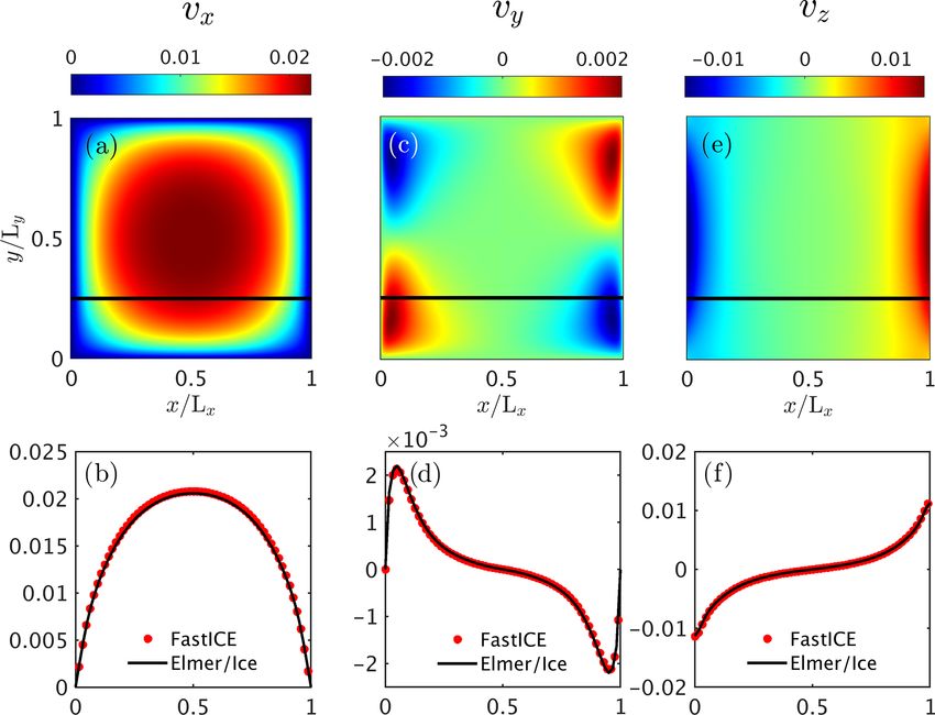
956                                                                          L. Räss et al.: Modelling thermomechanical ice

grounding zones and the basal interface. These boundaries          This principle entails every single instruction being executed
dictate the stability of the current main drainage routes from     on different data. The same instruction block is executed by
Antarctica and Greenland, and predicting their future evolu-       every thread. GPUs’ massive parallelism and the related high
tion is critical for understanding polar ice-sheet discharge.      performance is achieved by executing thousands of threads
   Full Stokes models (Gagliardini and Zwinger, 2008;              concurrently using multi-threading in order to effectively
Gagliardini et al., 2013; Jarosch, 2008; Jouvet et al., 2008;      hide latency. Numerical stencil-based techniques such as the
Larour et al., 2012; Leng et al., 2012, 2014; Brinkerhoff and      finite-difference method allow one to take advantage of GPU
Johnson, 2013; Isaac et al., 2015) provide a complete me-          hardware, since spatial derivatives are approximated by dif-
chanical description of deformation by capturing the entire        ferences between two (or more) adjacent grid points. This re-
stress rate and strain rate tensor. In three dimensions (3-D),     sults in minimal, local and regular memory access patterns.
full Stokes calculations set a high demand on computational        The operations performed on each stencil are identical for
resources that requires a parallel and high-performance com-       each grid point throughout the entire computational domain.
puting approach to achieve reasonable times to solution. An        Combined with a matrix-free discretisation of the equations
added challenge in full Stokes models is the strongly non-         and iterative PT updates, the finite-difference stencil evalu-
linear thermomechanics of ice. Ice viscosity significantly de-     ation is well suited for the SIMD programming philosophy
pends on both temperature and strain rate (Robin, 1955; Hut-       of GPUs. Each operation on the GPU assigns one thread to
ter, 1983; Morland, 1984), which can lead to spontaneous           compute the update of a given grid point. Since on the GPU
localisation of shear (e.g. Duretz et al., 2019; Räss et al.,      device, one core can simultaneously execute several threads,
2019a). Particularly challenging is the scale separation asso-     the operation set is executed on the entire computational do-
ciated with localisation, which leads to microscale physical       main almost concurrently.
interaction generating mesoscale features such as thermally           We tailor our numerical method to optimally exploit the
activated shear zones or preferential flow paths in macroscale     massive parallelism of GPU hardware, taking inspiration
ice domains. Thus, both high spatial and temporal resolutions      from recent successful GPU-based implementations of vis-
are important for numerical models to capture and resolve          cous and coupled flow problems (Omlin, 2017; Räss et al.,
spontaneous localisation.                                          2018, 2019a; Duretz et al., 2019). Our work is most compara-
   The main contribution of this paper is to leverage the          ble to the few land–ice dynamical cores targeting many-core
unprecedented parallel performance of modern graphical             architectures such as GPUs (Brædstrup et al., 2014; Watkins
processing units (GPUs) to accelerate the time to solution         et al., 2019). Our numerical implementation relies on an it-
for thermomechanically coupled full Stokes models in 3-            erative and matrix-free method to solve the mechanical and
D utilising a pseudo-transient (PT) iterative scheme – Fas-        thermal problems using a finite-difference discretisation on
tICE (Räss et al., 2019b). FastICE is a process-based model        a Cartesian staggered grid. We ensure optimal performance,
that focuses specifically on improving our ability to bet-         minimising the memory footprint bottleneck while ensuring
ter model and understand spontaneous englacial instabilities       optimal data alignment in computer memory. Our acceler-
such as thermomechanical localisation at the scale of individ-     ated PT algorithm (Frankel, 1950; Cundall et al., 1993; Poli-
ual field sites. Thermomechanical localisation arises in a self-   akov et al., 1993; Kelley and Keyes, 1998; Kelley and Liao,
consistent way in shear margins, at the grounding zone and in      2013) utilises an analogy of transient physics to converge
the vicinity of the basal sliding interface, making our model      to the steady-state problem at every time step. One advan-
particularly well suited for assessing the complex physical        tage of this approach is that the iterative stability criterion
feedbacks in the boundaries of fast-moving ice. FastICE is a       is physically motivated and intuitive to adjust and to gener-
complement to existing models by providing a multi-physics         alise. Using transient physics for numerical purposes allows
platform for studying the transition between fast and slow ice     us to define local CFL-like (Courant–Friedrich–Lewy) crite-
motion rather than addressing the large-scale evolution of the     ria in each computational cell to be used to minimise resid-
entire ice sheet.                                                  uals. This approach enables a maximal convergence rate si-
   Recent trends in the computing industry show a shift from       multaneously in the entire domain and avoids costly global
single-core to many-core architectures as an effective way to      reduction operations from becoming a bottleneck in parallel
increase computational performance. This trend is common           computing.
to both central processing unit (CPU) and GPU hardware ar-            We verify the numerical implementation of our mechan-
chitectures (Cook, 2012). GPUs are compact, affordable and         ical Stokes solver against available benchmark studies in-
relatively programmable devices that offer high-performance        cluding EISMINT (Huybrechts and Payne, 1996) and IS-
throughput (close to TB per second peak memory through-            MIP (Pattyn et al., 2008). There is only one model inter-
put) and a good price-to-performance ratio. GPUs offer an          comparison that investigates the coupled thermomechanical
attractive alternative to conventional CPUs owing to their         dynamics, EISMINT 2 (Payne et al., 2000). Unfortunately,
massively parallel architecture featuring thousands of cores.      experiments in EISMINT 2 are usually performed using
The programming model behind GPUs is based on a paral-             a coupled thermomechanical first-order shallow ice model
lel principle called single instruction multiple data (SIMD).      (Payne and Baldwin, 2000; Saito et al., 2006; Hindmarsh,

Geosci. Model Dev., 13, 955–976, 2020                                                 www.geosci-model-dev.net/13/955/2020/
L. Räss et al.: Modelling thermomechanical ice                                                                                                                     957

2006, 2009; Bueler et al., 2007; Brinkerhoff and Johnson,                   where T represents the temperature deviation from the initial
2015), making the comparison to our full Stokes implemen-                   temperature T0 , c is the specific heat capacity, k is the spa-
tation less immediate. Although thermomechanically cou-                     tially varying thermal conductivity and ˙ij is the strain rate
pled Stokes models exist (Zwinger et al., 2007; Leng et al.,                tensor. The term τij ˙ij represents the shear heating, a source
2014; Schäfer et al., 2014; Gilbert et al., 2014; Zhang et al.,             term that emerges from the mechanical model.
2015; Gong et al., 2018), very few studies have investigated                   Shear heating could locally raise the temperature in the ice
key aspects of the implemented model, such as convergence                   to the pressure melting point. Once ice has reached the melt-
among grid refinement and impacts of one-way vs. two-way                    ing point, any additional heating is converted to latent heat,
couplings, with few exceptions (e.g. Duretz et al., 2019).                  which prevents further temperature increase. Thus, we im-
   We start by providing an overview of the mathematical                    pose a temperature cap at the pressure melting point, follow-
model, describing ice dynamics and its numerical implemen-                  ing Suckale et al. (2014), by describing the melt production
tation. We then discuss GPU capabilities and explain our                    using a Heaviside function χ (T − Tm ):
GPU implementation. We further report model comparison
                                                                                     ∂T      ∂T             ∂            ∂T
against a selection of benchmark studies, followed by shar-                 ρc          + vi           =             k             + [1 − χ (T − Tm )]τij ˙ij ,   (4)
                                                                                     ∂t      ∂xi           ∂xi           ∂xi
ing the results and performance measurements. Finally, we
discuss pros and cons of the method and highlight glacio-                   where Tm stands for the ice melting temperature. We balance
logical contexts in which our model could prove useful. The                 the heat produced by shear heating with a sink term in re-
code examples based on the PT method in both the MATLAB                     gions where the melting temperature is reached. The volume
and CUDA C programming language are available for down-                     of produced meltwater can be calculated in a similar way as
load from Bitbucket at: https://bitbucket.org/lraess/fastice/               proposed by Suckale et al. (2014).
(last access: 2 March 2020) and from: http://wp.unil.ch/                       We approximate the rheology of ice through Glen’s flow
geocomputing/software/ (last access: 2 March 2020).                         law (Glen, 1952; Nye, 1953):

                                                                                                    ∂vj

                                                                                      1       ∂vi                                              Q
                                                                            ˙ij =                +            = a0 τII n−1 exp −                        τij ,     (5)
                                                                                      2       ∂xj   ∂xi                                     R(T + T0 )
2     The model
                                                                            where a0 is the pre-exponential factor, R is the universal gas
2.1      The mathematical model                                             constant, Q is the activation energy, n is the stress exponent
                                                                            and τIIpis the second invariant of the stress tensor defined by
We capture the flow of an incompressible, non-linear, viscous
                                                                            τII = 1/2τij τij . Glen’s flow law posits an exponent of n =
fluid – including a temperature-dependent rheology. Since
                                                                            3.
ice is approximately incompressible, the equation for con-
                                                                               At the ice-top surface 0t (t), we impose the upper surface
servation of mass reduces to
                                                                            boundary condition σij nj = −Patm nj , where nj denotes the
∂vi                                                                         normal unit vector at the ice surface boundary and Patm the
    =0,                                                               (1)   atmospheric pressure. Because atmospheric pressure is neg-
∂xi
                                                                            ligible relative to pressure within the ice column, we can also
where vi is the velocity component in the spatial direction xi .            use a standard stress-free simplification of the upper surface
  Neglecting inertial forces, ice’s flow is driven by gravity               boundary condition σij nj = 0. On the bottom ice–bedrock
and is resisted by internal deformation and basal stress:                   interface, we can impose two different boundary conditions.
                                                                            For the parts of the ice–bedrock interface 00 (t) where the
∂τij   ∂P                                                                   ice is frozen to the ground, we impose a zero velocity vi = 0
     −     + Fi = 0 ,                                                 (2)
∂xj    ∂xi                                                                  and thus no sliding boundary condition. On the parts of the
                                                                            ice–bedrock interface 0s (t) where the ice is at the melting
where Fi = ρg sin(α)[1, 0, − cot(α)] is the external force.                 point, we impose a Rayleigh friction boundary condition –
Ice density is denoted by ρ, g is the gravitational accelera-               the so-called linear sliding law – given by
tion and α is the characteristic bed slope. P is the isotropic
pressure and τij is the deviatoric stress tensor. The devia-                vi ni = 0 ,
toric stress tensor τij is obtained by decomposing the Cauchy               ni σij tj = −β 2 vj tj ,                                                               (6)
stress tensor σij in terms of deviatoric stress τij and isotropic
pressure P .                                                                where the parameter β 2 denotes a given sliding coefficient,
   In the absence of phase transitions, the temporal evolution              ni denotes the normal unit vector at the ice–bedrock inter-
of temperature in deforming, incompressible ice is governed                 face and tj denotes any unit vector tangential to the bottom
by advection, diffusion and shear heating:                                  surface. On the side or lateral boundaries, we impose either
                                                                            Dirichlet boundary conditions if the velocities are known or

         ∂T      ∂T             ∂            ∂T                             periodic boundary conditions, mimicking an infinitely ex-
ρc          + vi           =             k             + τij ˙ij ,   (3)   tended domain.
         ∂t      ∂xi           ∂xi           ∂xi

www.geosci-model-dev.net/13/955/2020/                                                                      Geosci. Model Dev., 13, 955–976, 2020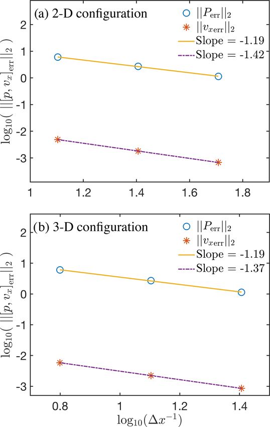
958                                                                                L. Räss et al.: Modelling thermomechanical ice

2.2     Non-dimensionalisation

For numerical purposes and for ease of generalisation, it is      ∂vi0
                                                                       =0,
often preferable to use non-dimensional variables. This al-       ∂xi0
lows one to limit truncation errors (especially relevant for
                                                                  ∂τij0        ∂P 0
single-precision calculations) and to scale the results to var-           −         + Fi0 = 0 ,
ious different initial configurations. Here, we use two dif-      ∂xj0         ∂xi0
ferent scale sets, depending on whether we solve the purely       ∂T 0           0   ∂ 2T 0
                                                                            0 ∂T
mechanical part of the model or the thermomechanically cou-             + v i    0 =        + τij0 ˙0 ij ,
                                                                   ∂t 0       ∂xi    ∂xi0 2
pled system of equations.
                                                                                      ∂vj0
                                                                                            !
   In the case of an isothermal model, we use ice thickness,      ˙0      1 ∂vi0
H , and gravitational driving stress to non-dimensionalise the     ij =            + 0
                                                                          2 ∂xj0      ∂xi
governing equations:
                                                                                              nT 0

                                                                           −n 0 n−1
                                                                        = 2 τII      exp             0    τij0 ,                 (10)
L=H ,                                                                                        1 + TT 0
                                                                                                                0
τ = ρgL sin(α), ,
v = 2n A0 Lτ n ,                                           (7)    where Fi0 is now defined as Fi0 = F [1, 0, − cot(α)] and
                                                                  F = ρg sin(α)L/τ . The model parameters are the non-
where A0 is the isothermal deformation rate factor and α is       dimensional initial temperature T00 , the stress exponent n,
the mean bed slope. We can then rewrite the governing equa-       the non-dimensional force F , the mean bed slope α, non-
tions in their non-dimensional form as follows:                   dimensional domain height L0z , and the horizontal domain
                                                                  size L0x and L0y (Fig. 3). We motivate the chosen characteris-
∂vi0                                                              tic scales by their usage in other studies of thermomechani-
     =0,
∂xi0                                                              cal strain localisation (Duretz et al., 2019; Kiss et al., 2019).
∂τij0    ∂P 0                                                     In the interest of a simple notation, we will omit the prime
        −     + Fi0 = 0 ,                                         symbols on all non-dimensional variables in the remainder
 ∂xj0    ∂xi0                                                     of the paper.
                    ∂vj0
                         !
            ∂v 0
        1                       n−1 0
˙ ij =
  0            i
                 + 0 = 2−n τII0    τij ,                   (8)    2.3     A simplified 1-D semi-analytical solution
        2 ∂xj0      ∂xi
                                                                  We consider a specific 1-D mathematical case in which all
where Fi0 is now defined as Fi0 = [1, 0, − cot(α)]. The model
                                                                  horizontal derivatives vanish (∂/∂x = ∂/∂y = 0). The only
parameters are the mean bed slope α and domain size in each
                                                                  remaining shear stress component τxz and pressure P are de-
horizontal direction, i.e. L0x and L0y .
                                                                  termined by analytical integration and are constant in time
   Reducing the thermomechanically coupled equations to a
                                                                  considering a fixed domain. We assume that stresses vanish
non-dimensional form requires not only length and stress,
                                                                  at the surface, and we set both horizontal and vertical basal
but also temperature and time. We choose the characteris-
                                                                  velocity components to 0. We then integrate the 1-D mechan-
tic scales such that the coefficients in front of the diffusion
                                                                  ical equation in the vertical direction and substitute it into the
and shear heating terms in the temperature evolution Eq. (3)
                                                                  temperature equation, which leads to
reduce to 1:

    nRT0 2                                                        ∂T (z, t) ∂ 2 T (z, t)                 (n+1)
T =        ,                                                               =       2
                                                                                         + 2(1−n) F Lz
      Q                                                              ∂t         ∂z
                                                                          (n+1)
τ = ρcp T ,                                                              z                nT (z, t)
                                                                    1−            exp                  ,

                         Q
                                                                       Lz               1 + T (z,t)
                                                                                               T0
t = 2−n a0−1 τ −n exp         ,
                        RT0                                                                                 Zz             n
                                                                                    (1−n)
                                                                                                       n              z
                                                                  vx (z, t) = 2                 F Lz                1−
    s
       k                                                                                                               Lz
L=         t.                                              (9)                                              0
      ρcp
                                                                              nT (z, t)
                                                                  exp                           dz .                             (11)
These choices entail the velocity scale in the thermomechan-                  1 + T (z,t)
                                                                                    T0
ical model being v = L/t. We obtain the non-dimensional
(primed variables) by using the characteristic scales given in    Notably, the velocity and shear heating terms (Eq. 11) are
Eq. (9), which leads to                                           now a function only of temperature and thus of depth and
                                                                  time. To obtain a solution to the coupled system, one only

Geosci. Model Dev., 13, 955–976, 2020                                                           www.geosci-model-dev.net/13/955/2020/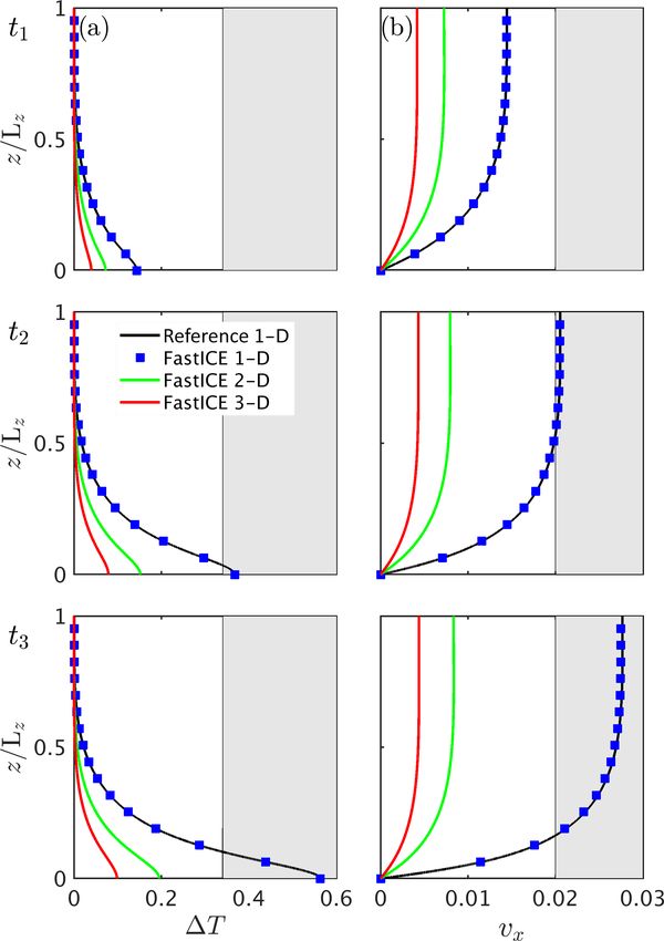
L. Räss et al.: Modelling thermomechanical ice                                                                                      959

needs to numerically solve for the temperature evolution pro-
file, while the velocity can then be obtained diagnostically by
a simple numerical integration.

2.4   The numerical implementation

We discretise the coupled thermomechanical Stokes equa-
tions (Eq. 10) using the finite-difference method on a stag-
gered Cartesian grid. Among many numerical methods cur-
rently used to solve partial differential equations, the finite-
difference method is commonly used and has been success-
fully applied in solving a similar equation set relating to
geophysical problems in geodynamics (Harlow and Welch,
                                                                    Figure 1. Setup of the staggered grid in 2-D. Variable C is located
1965; Ogawa et al., 1991; Gerya, 2009). The staggering              at the cell centre, V depicts variables located at cell vertices, and
of the grid provides second-order accuracy of the method            Mx and My represent variables located at cell mid-faces in the x or
(Virieux, 1986; Patankar, 1980; Gerya and Yuen, 2003; Mc-           y direction.
Kee et al., 2008), avoids oscillatory pressure modes (Shin
and Strikwerda, 1997) and produces simple yet highly com-
pact stencils. The different physical variables are located at         We rely on a pseudo-transient (PT) continuation or relax-
different locations on the staggered grid. Pressure nodes and       ation method to solve the system of coupled non-linear par-
normal components of the strain rate tensor are located at          tial differential equations (Eq. 10) in an iterative and matrix-
the cell centres. Velocity components are located at the cell       free way (Frankel, 1950; Cundall et al., 1993; Poliakov et al.,
mid-faces (Fig. 1), while shear stress components are located       1993; Kelley and Keyes, 1998; Kelley and Liao, 2013). To
at the cell vertices in 2-D (e.g. Harlow and Welch, 1965).          this end, we reformulate the thermomechanical Eq. (10) in a
The resulting algorithms are well suited for taking advantage       residual form:
of modern many-core parallel accelerators, such as graphi-
cal processing units (GPUs) (Omlin, 2017; Räss et al., 2018,           ∂vi
2019a; Duretz et al., 2019). Efficient parallel solvers utilis-     −      = fp ,
                                                                       ∂xi
ing modern hardware provide a viable solution to resolve the
                                                                    ∂τij   ∂P
computationally challenging coupled thermomechanical full                −     + Fi = fvi ,
Stokes calculations in 3-D. The power-law viscous ice rhe-          ∂xj    ∂xi
ology (Eq. 5) exhibits a non-linear dependence on both the              ∂T      ∂T   ∂ 2T
temperature and the strain rate:                                    −      − vi    +      + τij ˙ij = fT .                         (13)
                                                                        ∂t      ∂xi ∂xi 2
                                !
        1−n            T                                            The right-hand-side terms (fp , fvi , fT ) are the non-linear
η = ˙II n    exp −        T
                                    ,                       (12)    continuity, momentum and temperature residuals, respec-
                      1+   T0                                       tively, and quantify the magnitude of the imbalance of the
                                                                    corresponding equations.
where ˙II is the squareproot of the second invariant of the           We augment the steady-state equations with PT terms us-
strain rate tensor ˙II = 1/2˙ij ˙ij . We regularise the strain   ing the analogy of physical transient processes such as the
rate and temperature-dependent viscosity η to prevent non-          bulk compressibility or the inertial terms within the momen-
physical values for negligible strain rates, ηreg = 1/(η−1 +        tum equations (Duretz et al., 2019). This formulation enables
η0−1 ). We use a harmonic mean to obtain a naturally smooth         us to integrate the equation forward in pseudo-time τ until we
transition to background viscosity values at negligible strain      reach the steady state (i.e. the pseudo-time derivatives van-
rate η0 .                                                           ish). Relying on transient physics within the iterative process
   We define temperature on the cell centres within our stag-       provides well-defined (maximal) iterative time step limiters.
gered grid. We discretise the temperature equation’s advec-         We reformulate Eq. (10):
tion term using a first-order upwind scheme, doing the phys-
ical time integration using either an implicit backward Euler          ∂vi   ∂P
or a Crank–Nicolson (Crank and Nicolson, 1947) scheme.              −      =     ,
                                                                       ∂xi   ∂τp
To ensure that our numerical results are not confounded by
numerical diffusion, the grid Peclet number must be smaller         ∂τij   ∂P         ∂vi
                                                                         −     + Fi =      ,
than the physical Peclet number. Limiting numerical diffu-          ∂xj    ∂xi        ∂τvi
sion is one motivation for using high numerical resolution in           ∂T      ∂T   ∂ 2T               ∂T
our computations.                                                   −      − vi    +     2
                                                                                           + τij ˙ij =     ,                       (14)
                                                                        ∂t      ∂xi ∂xi                 ∂τT

www.geosci-model-dev.net/13/955/2020/                                                     Geosci. Model Dev., 13, 955–976, 2020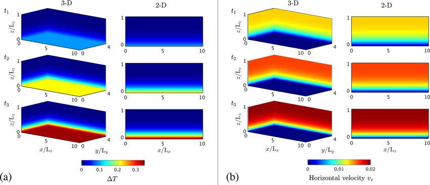
960                                                                             L. Räss et al.: Modelling thermomechanical ice

where we introduced the pseudo-time derivatives ∂/∂τ for            cosity. This interdependence reduces the iterative method’s
the continuity (∂P /∂τp ), the momentum (∂vi /∂τvi ) and the        sensitivity to the variations in the ice’s viscosity.
temperature (∂T /∂τT ) equation.                                       During the iterative procedure, we allow for finite com-
   For every non-linear iteration k, we update the effective        pressibility in the ice, ∂P /∂τp , while ensuring that the PT
viscosity ηeff [k] in the logarithmic space by taking a fraction    iterations eventually reach the incompressible solution. The
θη of the actual physical viscosity η[k] using the current strain   relaxation of the incompressibility constraint is analogous
rate and temperature solution fields and a fraction (1 − θη )       to the penalisation of pressure pioneered by Chorin (1967,
of the effective viscosity calculated in the previous iteration     1968) and subsequently extended by others. Compared to
ηeff [k−1] :                                                        projection-type methods, it has the advantage that no pres-
              h                                  i              sure boundary condition is necessary that will lead to nu-
ηeff [k] = exp θη ln η[k] + (1 − θη ) ln ηeff [k−1] .        (15)   merical boundary layers (Weinan and Liu, 1995). We use
                                                                    the parameter ηb to balance the divergence-free formulation
We use the scalar θη (0 ≤ θη ≤ 1) to select the fraction of a       of strain rates in the normal stress component evaluation,
given non-linear quantity, here the effective viscosity ηeff , to   wherein it is multiplied with the pressure residual fp . Thus,
be updated each iteration. When θη = 0, we would always             normal stress is given by τii = 2η(˙ii + ηb fp ). With conver-
use the initial guess, while for θη = 1, we would take 100%         gence of the method, the pressure residual fp vanishes and
of the current non-linear quantity. We usually define theta         the incompressible form of the normal stresses is recovered.
to be in the range of 10−2 − 10−1 in order to account for              Combining the residual notation introduced in Eq. (13)
some time to fully relax the non-linear viscosity as the non-       with the pseudo-time derivatives in Eq. (14) leads to the up-
linear problem may not be sufficiently converged at the be-         date rules:
ginning of the iterations. This approach is in a way similar
to an under-relaxation scheme and was successfully imple-           P [k] = P [k−1] + 1P [k] ,
mented in the ice-sheet model development by Tezaur et al.          vi [k] = vi [k−1] + 1vi [k] ,
(2015), for example.
                                                                    T [k] = T [k−1] + 1T [k] ,                                (17)
   The pseudo-time integration of Eq. (14) leads to the defi-
nition of pseudo-time steps 1τp , 1τvi and 1τT for the con-         where the pressure, velocity and temperature iterative incre-
tinuity, momentum and temperature equations, respectively.          ments represent the current residual [k] multiplied by the
Transient physical processes such as compressibility (conti-        pseudo-time step:
nuity equation) or acceleration (momentum equation) dictate
the maximal allowed explicit pseudo-time step to be utilised        1P [k] = 1τp fp [k] ,
in the transient process. Using the largest stable steps al-
lows one to minimise the iteration count required to reach          1vi [k] = 1τvi fvi [k] ,
the steady state:                                                   1T [k] = 1τT fT [k] .                                     (18)
                   k (1 + η )
         2.1 ndim ηeff     b                                           The straightforward update rule (Eq. 17) is based on a
1τp =                         ,                                     first-order scheme (∂/∂τ ). In 1-D, it implies that one needs
               max(ni )
                                                                    N 2 iterations to converge to the stationary solution, where
             min(1xi )2
1τvi =                      ,                                       N stands for the total number of grid points. This behaviour
                k (1 + η )
      2.1 ndim ηeff     b                                           arises because the time step limiter 1τvi implies a second-
                       1 −1                                         order dependence on the spatial derivatives for the strain

         2.1ndim
1τT =               +         ,                             (16)    rates. In contrast, a second-order scheme (Frankel, 1950),
        min(1xi )2 1t
                                                                     ψ∂ 2 /∂τ 2 + ∂/∂τ invokes a wave-like transient physical
where ndim is the number of dimensions, and 1xi and ni are          process for the iterations. The main advantage is the scaling
the grid spacing and the number of grid points in the i di-         of the limiter as 1x instead of 1x 2 in the explicit pseudo-
rection (i = x in 1-D, x, z in 2-D and x, y, z in 3-D), respec-     transient time step definition. We can reformulate the veloc-
tively. The physical time step, 1t, advances the temperature        ity update as
in time. The pseudo-time step 1τT is an explicit Courant–
Friedrich–Lewy (CFL) time step that combines temperature            1vi [k] = 1τvi fvi [k]
advection and diffusion. Similarly, 1τvi is the explicit CFL

                                                                             ν
time step for viscous flow, representing the diffusion of strain    + 1−          1vi [k−1] ,                                 (19)
                                                                             ni
rates with viscosity as the diffusion coefficient. It is modified
to account for the numerical equivalent of a bulk viscosity         where ψ can be expanded to (1−ν/ni ) and acts like a damp-
ηb . We choose 1τp to be the inverse of 1τvi to ensure that         ing term on the momentum residual. A similar damping ap-
the pressure update is proportional to the effective viscosity,     proach is used for elastic rheology in the FLAC (Cundall
while the velocity update is sensitive to the inverse of the vis-   et al., 1993) geotechnical software in order to significantly

Geosci. Model Dev., 13, 955–976, 2020                                                    www.geosci-model-dev.net/13/955/2020/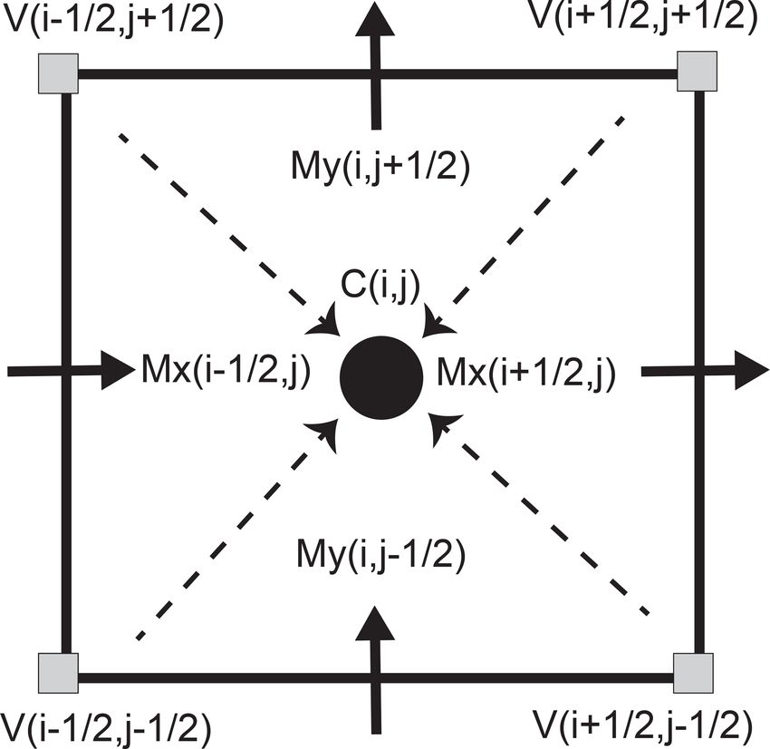
L. Räss et al.: Modelling thermomechanical ice                                                                                   961

                                                                     sic parallelism of shared memory devices, particularly tar-
                                                                     geting GPUs. A GPU is a massively parallel device origi-
                                                                     nally devoted to rendering the colour values for pixels on a
                                                                     screen independently from one another whereby the latency
                                                                     can be masked by high throughput (i.e. compute as many jobs
                                                                     as possible in a reasonable time). A schematic representa-
                                                                     tion (Fig. 2) highlights the conceptual discrepancy between a
                                                                     GPU and CPU. On the GPU chip, most of the area is devoted
Figure 2. Schematic chip representation for both the central pro-    to the arithmetic units, while on the CPU, a large area of the
cessing unit (CPU) and graphical processing unit (GPU) architec-     chip hosts scheduling and control microsystems.
ture. The GPU architecture consists of thousands of arithmetic and      The development of GPU-based solvers requires time to
logical units (ALUs). On the CPU, most of the on-chip space is de-   be devoted to the design of new algorithms that leverage the
voted to controlling units and cache memory, while the number of     massively parallel potential of the current GPU architectures.
ALUs is significantly reduced.                                       Considerations such as limiting the memory transfers to the
                                                                     mandatory minimum, avoiding complex data layouts, prefer-
                                                                     ring matrix-free solvers with low memory footprint and op-
reduce the number of iterations needed for the algorithm             timal parallel scalability instead of classical direct–iterative
to converge. The optimal value of the introduced parame-             solver types (Räss et al., 2019a) are key in order to achieve
ter ν is found to be in a range (1 ≤ ν ≤ 10), and it is usu-         optimal performance.
ally problem-dependent. This approach was successfully im-              Our implementation does not rely on the CUDA unified
plemented in recent PT developments by Räss et al. (2018,            virtual memory (UVM) features. UVM avoids the need to
2019a) and Duretz et al. (2019). The iteration count increases       explicitly define data transfers between the host (CPU) and
with the numerical problem size for second-order PT solvers          device (GPU) arrays but results in about 1 order of magnitude
and scales close-to-ideal multi-grid implementations. How-           lower performance. We suspect the internal memory han-
ever, the main advantage of the PT approach is its concise-          dling to be responsible for continuously synchronising the
ness and the fact that only one additional read/write operation      host and device memory, which is not needed in our case.
needs to be included – keeping additional memory transfers
to the strict minimum.                                               3.2   Multi-GPU implementation
   Notably, the PT solution procedure leads to a two-way nu-
merical coupling between temperature and deformation (me-            We rely on a distributed memory parallelisation using the
chanics), which enables us to recover an implicit solution           message passing interface (MPI) library to overcome the on-
to the entire system of non-linear partial differential equa-        device memory limitation inherent to modern GPUs and ex-
tions. Besides the coupling terms, rheology is also treated          ploit supercomputers’ computing power. Access to a large
implicitly; i.e. the shear viscosity η is always evaluated using     number of parallel processes enables us to tackle larger com-
the current physical temperature, T , and strain rate, ˙II . Our    putational domains or to refine grid resolution. We rely on
method is fully local. At no point during the iterative pro-         domain decomposition to split our global computational do-
cedure does one need to perform a global reduction, nor to           main into local domains, each executing on a single GPU
access values that are not directly collocated. These consider-      handled by an MPI process. Each local process has its bound-
ations are crucial when designing a solution strategy that tar-      ary conditions defined by (a) physics if on the global bound-
gets parallel hardware such as many-core GPU accelerators.           ary or (b) exchanged information from the neighbouring pro-
We implemented the PT method in the MATLAB and CUDA                  cess in the case of internal boundaries. We use CUDA-aware
C programming languages. Computations in CUDA C can be               non-blocking MPI messages to exchange the internal bound-
performed in both double- and single-precision arithmetic.           aries among neighbouring processes. CUDA awareness al-
The computations in CUDA C shown in the remainder of the             lows us to bypass explicit buffer copies on the host mem-
paper were performed using double-precision arithmetic if            ory by directly exchanging GPU pointers, resulting in an
not specified otherwise.                                             enhanced workflow pipelining. Our algorithm implementa-
                                                                     tion and solver require no global reduction. Thus, there is
3     Leveraging hardware accelerators                               no need for global MPI communication, eliminating an im-
                                                                     portant potential scaling bottleneck. Although the proposed
3.1    Implementation on graphical processing units                  iterative and matrix-free solver features a high locality and
                                                                     should scale by construction, the growing number of MPI
Our GPU algorithm development effort is motivated by the             processes may deprecate the parallel runtime performance by
aim to resolve the coupled thermomechanical system of                about 20 % owing to the increasing number of messages and
equations (Eqs. 12–13) with high spatial and temporal ac-            overall machine occupancy (Räss et al., 2019c). We address
curacy in 3-D. To this end, we exploit the low-level intrin-         this limitation by overlapping MPI communication and the

www.geosci-model-dev.net/13/955/2020/                                                     Geosci. Model Dev., 13, 955–976, 2020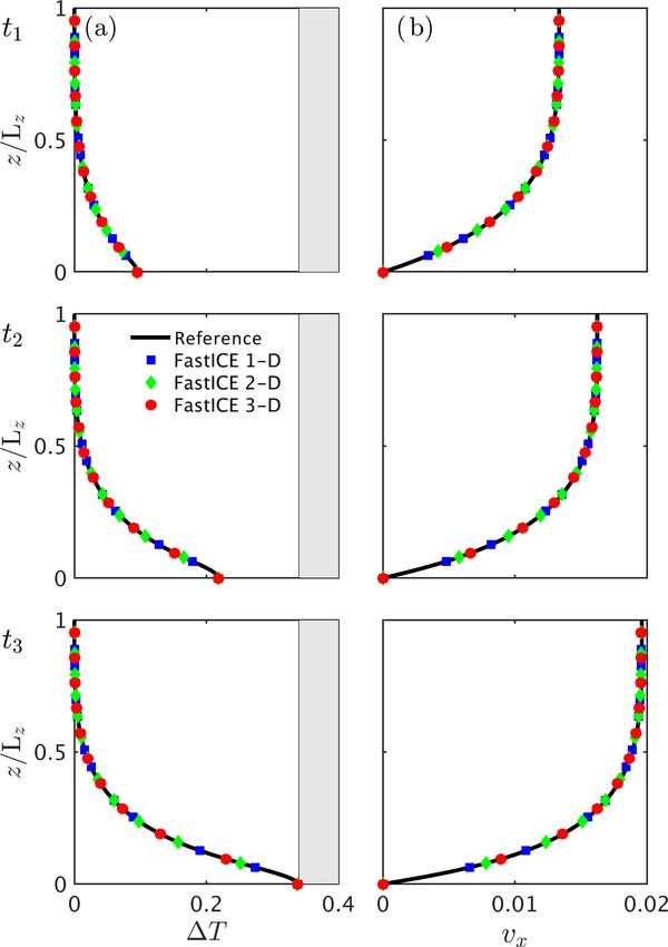
962                                                                             L. Räss et al.: Modelling thermomechanical ice

Figure 3. Model configuration for the numerical experiments: (a) 2-D model and (b) 3-D model. Both the surface and bed topography are
flat but inclined at a constant angle of α. We show both the model coordinate axes and the prescribed boundary conditions.

computation of the inner points of the local domains using
streams, a native CUDA feature. CUDA streams allow one
                                                                                            2π x
to assign asynchronous kernel execution and thus enable the          β 2 (x) = β0 1 + sin           ,
overlap between communication and computation, resulting                                     Lx

in optimal parallel efficiency.                                        2                      2π x       2πy
                                                                     β (x, y) = β0 1 + sin           sin        ,               (20)
                                                                                               Lx         Ly
4     The model configuration                                        where β0 is a chosen non-dimensional constant. Differences
                                                                     may arise depending on the prescribed values for the param-
To verify the numerical implementation of the developed              eters α, Lx , Ly and β0 . Experiment 2 represents the ISMIP
FastICE solver, we consider three numerical experiments              experiments C and D for L = 10 km (Pattyn et al., 2008), but
based on a box inclined at a mean slope angle of α. We per-          in our case using non-dimensional variables.
form these numerical experiments on both 2-D and 3-D com-               The mechanical part of Experiment 3 is analogous to Ex-
putational domains (Fig. 3a and b, respectively). The non-           periment 2. The boundary conditions are periodic in the
dimensional computational domains are 2−D = [0Lx ] ×                x and y directions unless specified otherwise. The thermal
[0Lz ] and 3−D = [0Lx ]×[0Ly ]×[0Lz ] for 2-D and 3-D do-           problem requires additional boundary conditions in terms of
mains, respectively. The difference between the 2-D and the          temperature or fluxes. We set the surface temperature T0 to
3-D configurations lies in the boundary conditions imposed           0. At the bottom, we set the vertical flux qz to 0 and, on the
at the base and at the lateral sides. At the surface, the zero       sides, we impose periodic boundary conditions. The model
stress σij nj = 0 boundary condition is prescribed in all ex-        parameters used in Experiment 3 are compiled in Table 2.
periments. Experiment 2’s model configuration corresponds            We employ the semi-analytical 1-D model (Sect. 2.3) as an
to the ISMIP benchmark (Pattyn et al., 2008), wherein exper-         independent benchmark for the Experiment 3 calculations.
iment C relates to the 3-D case and experiment D relates to
the 2-D case.
   Experiments 1 and 2 seek to first verify the implementa-          5     Results and performance
tion of the mechanical part of the Stokes solver, which is
the computationally most expensive part (Eq. 8). For these           5.1    Experiment 1: Stokes flow without basal sliding
experiments, we assume that the ice is isothermal and ne-
glect temperature. We compare our numerical solutions to             We compare our numerical solutions obtained with the GPU-
the solutions obtained by the commonly used finite-element           based PT method using a CUDA C implementation (Fas-
Stokes solver Elmer/Ice (Gagliardini et al., 2013), which has        tICE) to the reference Elmer/Ice model. We report all the
been thoroughly tested (Pattyn et al., 2008; Gagliardini and         values in their non-dimensional form, and the horizontal axes
Zwinger, 2008). Experiment 3 is a thermomechanically cou-            are scaled with their aspect ratio. We impose a no-slip bound-
pled case. The model parameters are the stress exponent n,           ary condition on all velocity components at the base and
the mean bed slope α, and the two horizontal distances Lx            prescribe free-slip boundary conditions on all lateral domain
and Ly in their respective dimensions (x, y), which appear in        sides. We prescribe a stress-free upper boundary in the verti-
Table 1. If a linear basal sliding law (Eq. 6) is prescribed, the    cal direction.
respective 2-D and 3-D sliding coefficients are                         In the 2-D configuration (Fig. 4), the horizontal velocity
                                                                     component vanishes at the left and right boundary, vx = 0,
                                                                     and thus the maximum velocity values in the horizontal di-
                                                                     rection are located in the middle of the slab. On the left
                                                                     side (x/Lx = 0), the ice is pushed down (compression); thus,

Geosci. Model Dev., 13, 955–976, 2020                                                   www.geosci-model-dev.net/13/955/2020/
L. Räss et al.: Modelling thermomechanical ice                                                                                             963

Table 1. Experiments 1 and 2: non-dimensional model parameters and the dimensional values D for comparison.


                                  Experiment       Lx      Ly         α    n         β0        LD
                                                                                                x      LD
                                                                                                        y       LD
                                                                                                                 z

                                  Exp. 1   2-D     10       –         10   3        –        2 km       –     200 m
                                  Exp. 1   3-D     10       4         10   3        –        2 km   800 m     200 m
                                  Exp. 2   2-D     10       –        0.1   3   0.1942       10 km       –      1 km
                                  Exp. 2   3-D     10      10        0.1   3   0.1942       10 km   10 km      1 km

Table 2. Experiment 3: non-dimensional model parameters and the dimensional values D for comparison.


              Experiment          Lx       Ly       Lz          α      n       F              T0     LD
                                                                                                      x       LD
                                                                                                               y       LD
                                                                                                                        z      T0D

              Exp. 3 1-D           –       –     3 × 10⁵        10     3   2.8 × 10⁻⁸        9.15      –         –    300 m   −10 ◦ C
              Exp. 3 2-D       10 Lz       –     3 × 10⁵        10     3   2.8 × 10⁻⁸        9.15   3 km         –    300 m   −10 ◦ C
              Exp. 3 3-D       10 Lz    4 Lz     3 × 10⁵        10     3   2.8 × 10⁻⁸        9.15   3 km    1.2 km    300 m   −10 ◦ C

                                                                               The DOFs represent three variables in 2-D (vx , vz , P ) and
                                                                               four variables in 3-D (vx , vy , vz , P ) multiplied by the num-
                                                                               ber of grid points involved.
                                                                                  We find good agreement between the two model solu-
                                                                               tions in the 3-D configuration as well (Fig. 5). We employed
                                                                               a numerical grid resolution of 319 × 159 × 119 grid points
                                                                               in the x, y and z directions (≈ 2.41 × 10⁷ DOFs) and used
                                                                               a numerical grid resolution of 61 × 61 × 21 (≈ 3.1 × 10⁵
                                                                               DOFs) in Elmer/Ice. Scaling our result to dimensional val-
                                                                               ues (Table 1) results in a maximal horizontal velocity (vx )
                                                                               of ≈ 105 m yr−1 . The horizontal distance is 2 km in the x di-
Figure 4. Comparison of the non-dimensional simulation results for             rection and 800 m in the y direction, and the ice thickness is
the 2-D configuration of Experiment 1. We show (a) the horizontal              200 m. The box is inclined at 10◦ .
component of the surface velocity, vx , and (b) the vertical compo-
nent of surface velocity, vz , across the ice slab for both our FastICE
model and Elmer/Ice. For context, the maximum horizontal veloc-                5.2        Experiment 2: Stokes flow with basal sliding
ity (vx ≈ 0.0365) corresponds to ≈ 174 m yr−1 . The horizontal dis-
tance is 2 km, while the ice thickness is 200 m. The box is inclined
at 10◦ .                                                                       We then consider the case in which ice is sliding at the base
                                                                               (ISMIP experiments C and D). We prescribe periodic bound-
                                                                               ary conditions at the lateral boundaries and apply a linear
                                                                               sliding law at the base. The top boundary remains stress-free
the vertical velocity values were negative. On the right side                  in the vertical direction.
(x/Lx = 1), the ice is pulled up (extension), and the vertical                    We performed the 2-D simulation of Experiment 2 (Fig. 6)
velocity values were positive. Our FastICE results agree well                  using a numerical grid resolution of 511×127 grid points (≈
with the numerical solutions produced by Elmer/Ice. The nu-                    1.95 × 10⁵ DOFs) for the FastICE solver and computed the
merical resolution of the Elmer/Ice model is 1001 × 275 grid                   Elmer/Ice solution using a numerical grid resolution of 241×
points in the x and z directions (≈ 8.25×10⁵ degrees of free-                  120 (≈ 8.7 × 10⁴ DOFs). We show both vx and vz velocity
dom – DOFs), while we employed 2047 × 511 grid points                          components at the slab’s surface. The two models’ results
(≈ 3.13 × 10⁶ DOFs) within our PT method. We use higher                        agree well.
numerical grid resolution within FastICE to jointly verify                        We performed the 3-D simulation of Experiment 2 (Fig. 7)
agreement with Elmer/Ice and convergence. The fact that we                     using a numerical grid resolution of 63 × 63 × 21 (≈ 3.33 ×
obtain matching results when increasing grid resolution sig-                   105 DOFs) for our FastICE solver and a numerical grid reso-
nificantly suggests that we have sufficiently resolved the rele-               lution of 61 × 61 × 21 (≈ 3.12 × 10⁵ DOFs) in the Elmer/Ice
vant physical processes, even at relatively low resolution. We                 model. In dimensional units, the maximum horizontal veloc-
report an exception to this trend in the 3-D case of Experi-                   ity (vx ) corresponds to ≈ 16.4 m yr−1 . The horizontal dis-
ment 2. The PT method’s efficiency enables simulations with                    tance is 10 km in the x direction 10 km in the y direction,
a large number of grid points without affecting the runtime.                   and the ice thickness is 1 km. The box is inclined at 0.1◦ .

www.geosci-model-dev.net/13/955/2020/                                                                  Geosci. Model Dev., 13, 955–976, 2020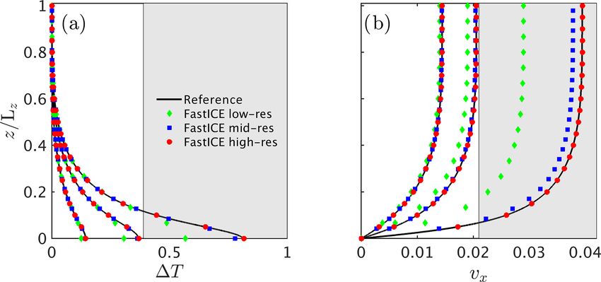
964 L. Räss et al.: Modelling thermomechanical ice
Figure 5. Non-dimensional simulation results for the 3-D configuration of Experiment 1. We report (a) the horizontal surface velocity
component vx , (c) the horizontal surface velocity component vy and (e) the vertical surface velocity component vz . The black solid line
depicts the position at which y = Ly /4. Panels (b), (d) and (f) show the surface velocity components vx , vy and vz , respectively, at y = Ly /4
and compare them against the results from the Elmer/Ice model.
iment 1 configuration owing to the periodicity on the lateral
boundaries.
We employ a matching numerical resolution between Fas-
tICE and Elmer/Ice in this particular benchmark case. Us-
ing higher resolution for FastICE results in minor discrep-
ancy between the two solutions, suggesting that the resolu-
tion in Fig. 7 is insufficient to capture small-scale physical
processes. We discuss this issue more in Sect. 5.5 where we
test the convergence of the FastICE numerical implementa-
tion upon grid refinement.
Figure 6. Non-dimensional simulation results for the 2-D configu- 5.3 Experiment 3a: thermomechanically coupled
ration of Experiment 2. We plot (a) the horizontal surface velocity Stokes flow without basal sliding
component vx and (b) the vertical surface velocity component vz
across the slab for both our FastICE model and Elmer/Ice. In di- We first verify that the 1-D, 2-D and 3-D model configura-
mensional terms, the maximum horizontal velocity (vx ≈ 5.58) cor- tions from Experiment 3 produce identical results, assum-
responds to ≈ 16.9 m yr−1 . The horizontal distance is 10 km, while ing periodic boundary conditions on all lateral sides. In this
the ice thickness is 1 km. The box is inclined at 0.1◦ . case, all the variations in the x or y directions vanish (∂/∂x
and ∂/∂y); thus, both the 2-D and 3-D models reduce to
the 1-D problem. We employ a numerical grid resolution
We find good agreement between the two numerical im- of 127 × 127 × 127 grid points in the x, y and z direction,
plementations. Since the flow is mainly oriented in the x di- 127 × 127 grid points in the x and z directions, and 127 grid
rection, the vy velocity component is more than 2 orders of points in the z direction for the 3-D, 2-D and 1-D problems,
magnitude smaller than the vx velocity component. Numeri- respectively.
cal errors in vy are more apparent than in the leading velocity We ensure that all results collapse onto the semi-analytical
component vx . We report a 1 order of magnitude increase in 1-D model solution (Sect. 2.3), which we obtained by ana-
the time to solution in Experiment 2 compared to the Exper- lytically integrating the velocity field and solving the decou-
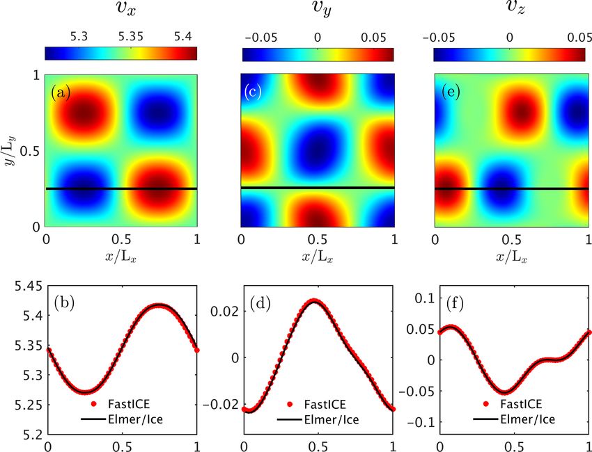
Geosci. Model Dev., 13, 955–976, 2020 www.geosci-model-dev.net/13/955/2020/L. Räss et al.: Modelling thermomechanical ice 965 Figure 7. Non-dimensional simulation results for the 3-D configuration of Experiment 2. We report (a) the horizontal surface velocity component vx , (c) the horizontal surface velocity component vy and (e) the vertical surface velocity component vz . The black solid line depicts the position at which y = Ly /4. Panels (b), (d) and (f) show the surface velocity components vx , vy and vz , respectively, at y = Ly /4 and compare them against the results from the Elmer/Ice model. pled thermal problem separately (Eq. 11). From a compu- correspond to a 300 m thick ice slab inclined at a 10◦ an- tational perspective, we numerically solve Eq. (11) using a gle with an initial surface temperature of −10 ◦ C. The max- high spatial and temporal accuracy and therefore minimise imum initial velocity for the isothermal ice slab corresponds the occurrence of numerical errors. We establish the 1-D ref- to ≈ 486 m yr−1 , while the maximum velocity just before erence solution for both the temperature and the velocity pro- the melting point is reached corresponds to 830 m yr−1 . The file, solving Eq. (11) on a regular grid, reducing the physi- comparison snapshot times are 1.6, 3.2 and 4.4 years. cal time steps until we converge to a stable reference solu- The semi-analytical 1-D solution enables us to evaluate tion. Our reference simulation involves 4000 grid points and the influence of the numerical coupling method and time a non-dimensional time step of 5 × 10⁵ (using a backward integration and to quantify when and why high spatial res- Euler time integration). We reach the total simulation time of olution is required in thermomechanical ice-flow simula- 2.9 × 10⁸ within 580 physical time steps. tions. We compare the 1-D semi-analytical reference solution We report overall good agreement of all model solutions (Eq. 11) to the results obtained with the 1-D FastICE solver (1-D, 2-D, 3-D and 1-D reference) at the three reported stages for three spatial numerical resolutions (nz = 31, 95 and 201 for this scenario (Fig. 8). As expected from the 1-D model grid points) at three non-dimensional times 1 × 10⁸ , 2 × 10⁸ solution, temperature varies only as a function of time and and 2.9 × 10⁸ (Fig. 10). The grey area in Fig. 10 highlights depth, with the highest value obtained close to the base and where the melting temperature is exceeded. Since our semi- for longer simulation times. Similarly, the velocity profile is analytical reference solution does not include phase transi- equivalent to the 1-D profile, and the largest velocity value tions, we also neglect this component in the numerical re- is located at the surface. We only report the horizontal veloc- sults. During the early stages of the simulation, the thermo- ity component vx for the 2-D and the 3-D models, since vy mechanical coupling is still minor, and solutions at all res- and vz feature negligible magnitudes. Thus, we only observe olution levels are in good agreement with one another and spatial variation in the vertical z direction. We report the non- with the reference. The low-resolution solution starts to devi- dimensional temperature T (Fig. 9a) and horizontal velocity ate from the reference (Fig. 10b) when the coupling becomes vx (Fig. 9b) fields for both the 3-D and the 2-D configura- more pronounced close to the thermal runaway point (Clarke tions compared at non-dimensional time 0.7 × 10⁸ , 1.4 × 10⁸ et al., 1977). The high-spatial-resolution solution is satisfac- and 1.9 × 10⁸ . The dimensional results from Experiment 3 tory at all stages. We conclude that high spatial resolution www.geosci-model-dev.net/13/955/2020/ Geosci. Model Dev., 13, 955–976, 2020
966 L. Räss et al.: Modelling thermomechanical ice
tion in physical time is performed using an implicit back-
ward Euler method for (1) and (2) and a forward Euler ex-
plicit time integration method for (3). We utilise the identical
non-dimensional time step for both the explicit and the im-
plicit numerical time integration. We perform 580 time steps,
reaching a simulation time of 2.9 × 10⁸ . We employ a verti-
cal grid resolution of nz = 201 grid points for all models. The
chosen time step for the explicit integration of the heat diffu-
sion equation is below the CFL stability condition given by
1z2 /2.1 in 1-D, where 1z represents the grid spacing in a
vertical direction.
Physically, the viscosity and shear heating terms are cou-
pled and are a function of temperature and strain rates, but we
update the viscosity and the shear heating term based on tem-
perature values from the previous physical time step. Thus,
the shear heating term can be considered a constant source
term in the temperature evolution equation during the time
step, leading to a semi-explicit rheology. We show the 1-D
numerical solutions of (blue) the fully coupled method with
a backward Euler (implicit) time integration and the two un-
coupled methods with either (green) backward (implicit) or
(red) forward (explicit) Euler time integration (Fig. 11) and
compare them to the 1-D reference model solution. Surpris-
ingly, and in contrast to Duretz et al. (2019), we observe a
good agreement between all methods, suggesting that the dif-
ferent coupling strategies capture the coupled flow physics
with sufficient accuracy given high enough spatial and tem-
poral resolution. However, for a longer-term evolution, the
uncoupled approaches may predict lower temperature and
Figure 8. Non-dimensional simulation results for (a) the temper- velocity values than the fully coupled approach.
ature deviation T and (b) the horizontal velocity component vx
for the 1-D, 2-D and 3-D FastICE models at three different non- 5.4 Experiment 3b: thermomechanically coupled
dimensional times 0.7 × 10⁸ , 1.4 × 10⁸ and 1.9 × 10⁸ compared to
Stokes flow in a finite domain
the 1-D reference model results. We employ a vertical grid resolu-
tion nz of 31, 95 and 201 grid points. We sample the 1-D profiles
at location x = Lx /2 in 2-D and at x = Lx /2 and y = Ly /2 in 3- Boundary conditions corresponding to immobile regions in
D. The shaded areas correspond to the part of the solution that is the computational domain may induce localisation of defor-
above the melting temperature, since we do not account for phase mation and flow observed in locations such as shear mar-
transitions in this case. gins, grounding zones or bedrock interactions. Dimensional-
ity plays a key role in such configurations, causing the stress
distribution to be variable among the considered directions.
is required to accurately capture the non-linear coupled be- We used the configuration in Experiment 3 to investigate
haviour in regimes close to the thermal runaway, which is the spatial variations in temperature and velocity distribu-
seldom the case in the models reported in the literature. tions by defining no-slip conditions on the lateral boundaries
Thermomechanical strain localisation may significantly for the mechanical problem and prescribing zero heat flux
impact the long-term evolution of a coupled system. A recent through those boundaries. We employ a numerical grid reso-
study by Duretz et al. (2019) suggested that partial coupling lution of 511 × 255 × 127 grid points, 511 × 127 grid points
may result in underestimating the thermomechanical locali- and 201 grid points for the 3-D, 2-D and 1-D case, respec-
sation compared to the fully coupled approach, as reported in tively. We prescribe a non-dimensional time step of 5 × 10⁵ .
their Fig. 8. We compare three coupling methods (Fig. 11): We perform 500 numerical time steps and reach a total non-
(1) a fully coupled implicit PT method, as described in the dimensional simulation time of 2.5 × 10⁸ . We then compare
numerical section, whereby the viscosity and the shear heat- the temperature T and horizontal velocity component vx at
ing term are implicitly determined by using the current guess; three times obtained with the 1-D, 2-D and 3-D FastICE
(2) an implicit numerically uncoupled mechanical and ther- solver to the reference solution (Fig. 12). We use 1-D profiles
mal model; and (3) an explicit numerically uncoupled me- for comparison, taken at location x = Lx /2 in the 2-D model
chanical and thermal model. The numerical time integra- and at location x = Lx /2 and y = Ly /2 in the 3-D model.
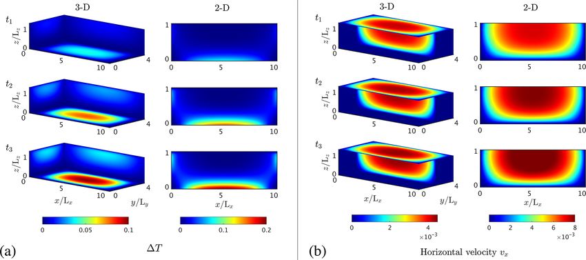
Geosci. Model Dev., 13, 955–976, 2020 www.geosci-model-dev.net/13/955/2020/L. Räss et al.: Modelling thermomechanical ice 967 Figure 9. Spatial distribution of (a) the temperature deviation from the initial temperature T and (b) the horizontal velocity component vx for 3-D (a) and 2-D (b) in non-dimensional units. We scale the domain extent with Lz . We compare the numerical solutions at non-dimensional times 0.7 × 10⁸ , 1.4 × 10⁸ and 1.9 × 10⁸ . Figure 10. Non-dimensional simulation results for (a) the temper- Figure 11. Non-dimensional simulation results for (a) the temper- ature deviation T and (b) the horizontal velocity component vx to ature deviation T and (b) the horizontal velocity component vx to test solver performance at three resolutions. The vertical resolutions evaluate different numerical time integration schemes. We consider are LR = 31, MR = 95 and HR = 201 grid points for low-, mid- three non-dimensional times 1 × 10⁸ , 2 × 10⁸ and 2.9 × 10⁸ and and high-resolution runs, respectively. We compare the results for compare our numerical estimates to the reference model. As before, non-dimensional time 1 × 10⁸ , 2 × 10⁸ and 2.9 × 10⁸ . The shaded the shaded areas correspond to the part of the solution that is above areas correspond to the part of the solution that is above the melting the melting temperature, since we neglect phase transitions in this temperature, since we do not account for phase transitions in this comparison. benchmark. We also report the temperature variation 1T (Fig. 13a) and are of the same order of magnitude as the 1-D shear stress the horizontal velocity component vx (Fig. 13b) for both the for the considered aspect ratio, reducing the horizontal ve- 2-D and 3-D simulations. The melting temperature approxi- locity vx in the 2-D and 3-D models. This also impacts the mately corresponds to 0.35 of the temperature deviation. The shear heating term, reducing the source term in the tempera- reported results correspond to a 2.3-, 4.6- and 5.8-year evo- ture evolution equation. In the 1-D configuration, the unique lution. shear stress tensor component is a function only of depth. On All three models start with identical initial conditions for the other endmember, the 3-D configurations allow for a spa- the thermal problem, i.e. 1T = 0 throughout the entire ice tially more distributed stress state. They lower strain rates in slab. The difference between the models arises owing to dif- this scenario and reduce the magnitude of shear heating in ferent stress distributions in 1-D, 2-D or 3-D. For instance, higher dimensions. The spatially heterogeneous temperature the additional stress components inherent in 2-D and 3-D and strain rate fields in all directions require the utilisation of www.geosci-model-dev.net/13/955/2020/ Geosci. Model Dev., 13, 955–976, 2020
You can also read