Properties of surface water masses in the Laptev and the East Siberian seas in summer 2018 from in situ and satellite data - Ocean Science
←
→
Page content transcription
If your browser does not render page correctly, please read the page content below
Ocean Sci., 17, 221–247, 2021
https://doi.org/10.5194/os-17-221-2021
© Author(s) 2021. This work is distributed under
the Creative Commons Attribution 4.0 License.

Properties of surface water masses in the Laptev and the East
Siberian seas in summer 2018 from in situ and satellite data
Anastasiia Tarasenko1,2,a , Alexandre Supply3 , Nikita Kusse-Tiuz1 , Vladimir Ivanov1 , Mikhail Makhotin1 ,
Jean Tournadre2 , Bertrand Chapron2 , Jacqueline Boutin3 , Nicolas Kolodziejczyk2 , and Gilles Reverdin3
1 Arcticand Antarctic Research Institute, Depatment of Oceanology, 199397 Saint Petersburg, Russia
2 Univ.Brest, CNRS, IRD, Ifremer, Laboratoire d’Océanographie Physique et Spatiale (LOPS), IUEM, Brest 29280, France
3 Sorbonne Université, CNRS, IRD, MNHN, Laboratoire d’Océanographie et du Climat,

Expérimentations et Approches Numériques (LOCEAN), 75005 Paris, France
a now at: Centre National de la Recherche Météorologique (CNRM), Université de Toulouse,

Météo-France, CNRS, 22300 Lannion, France

Correspondence: Anastasiia Tarasenko (tad.ocean@gmail.com)

Received: 31 May 2019 – Discussion started: 31 July 2019
Revised: 18 November 2020 – Accepted: 20 November 2020 – Published: 4 February 2021

Abstract. Variability of surface water masses of the Laptev       better understand the pathway of surface water displacement
and the East Siberian seas in August–September 2018 is            on the shelf and beyond.
studied using in situ and satellite data. In situ data were
collected during the ARKTIKA-2018 expedition and then
complemented with satellite-derived sea surface temperature
(SST), salinity (SSS), sea surface height, wind speed, and        1   Introduction
sea ice concentration. The estimation of SSS fields is chal-
lenging in high-latitude regions, and the precision of soil       The eastern part of the Eurasian Arctic remains one of the
moisture and ocean salinity (SMOS) SSS retrieval is im-           less studied areas of the Arctic Ocean. Carmack et al. (2016)
proved by applying a threshold on SSS weekly error. For           described this region as an “interior shelf” (the Kara sea,
the first time in this region, the validity of DMI (Danish        the Laptev sea, the East Siberian sea, and the Beaufort sea),
Meteorological Institute) SST and SMOS SSS products is            where 80 % of the Arctic basin river discharge is released.
thoroughly studied using ARKTIKA-2018 expedition con-             Armitage et al. (2016) estimated the annual river water in-
tinuous thermosalinograph measurements and conductivity–          put as 2000 m3 . The Arctic Ocean stores 11 % of global river
temperature–depth (CTD) casts. They are found to be ade-          discharge, and thus its role in a planetary water budget de-
quate to describe large surface gradients in this region. Sur-    serves a special attention. The surface stratification and the
face gradients and mixing of the river and the sea water in       freshwater content are regarded as key parameters that have
the ice-free and ice-covered areas are described with a spe-      to be followed to better understand the changing state of a
cial attention to the marginal ice zone at a synoptic scale. We   “New Arctic” climate (Carmack et al., 2016). Johnson and
suggest that the freshwater is pushed northward, close to the     Polyakov (2001) discussed the salinification of the Laptev
marginal ice zone (MIZ) and under the sea ice, which is con-      sea from 1989 up to 1997, explaining it as being due to the
firmed by the oxygen isotope analysis. The SST-SSS diagram        eastward freshwater displacement and an excessive brine re-
based on satellite estimates shows the possibility of investi-    lease in the sea ice leads. A more recent study reports that
gating the surface water mass transformation at a synoptic        a 20 % increase in the Eurasian river runoff has been ob-
scale and reveals the presence of river water on the shelf of     served over the last 40 years (Charette et al., 2020). Overall, a
the East Siberian Sea. The Ekman transport is calculated to       freshening of the American basin of the Arctic Ocean was re-
                                                                  ported in 2000–2010 (Carmack et al., 2016), and at the same
                                                                  time a decrease in a freshwater content of about 180 km3 be-

Published by Copernicus Publications on behalf of the European Geosciences Union.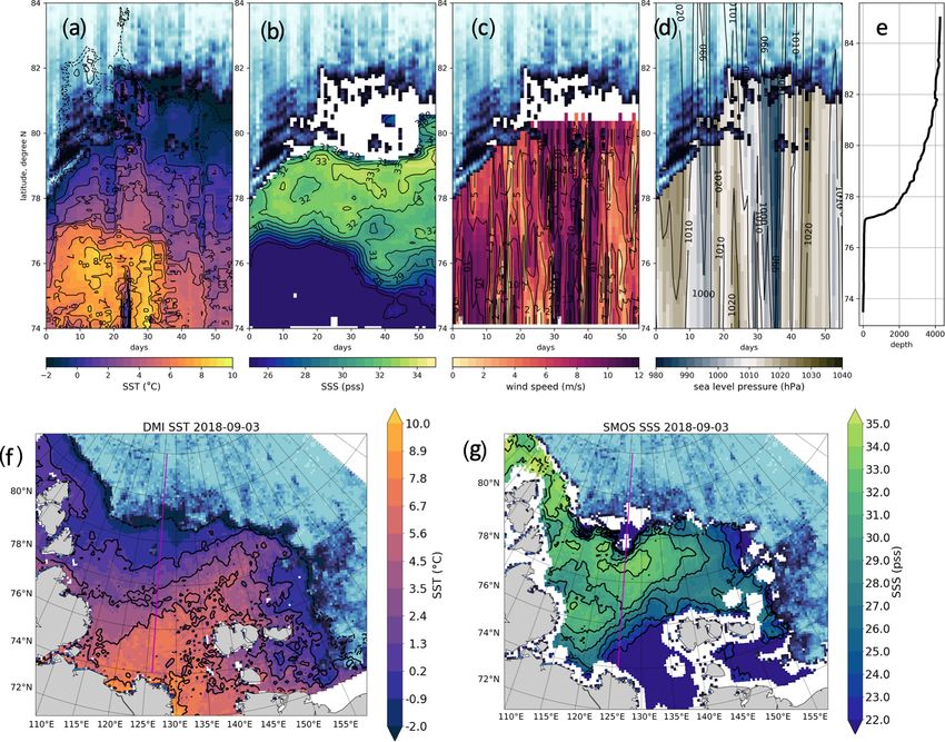
222                                                 A. Tarasenko et al.: Properties of surface water masses in the Laptev Sea

tween 2003 and 2014 was calculated from altimetry measure-              The Laptev Sea is shallow in its southern and central parts
ments by Armitage et al. (2016) over the Siberian shelf. The         (less than 100 m) with a very deep opening in the north
importance of shelf seas for the freshwater content storage          (3000 m) (Fig. 1). Several water masses are mixed in the
and distribution was outlined in several recent studies (Haine       Laptev Sea. The Lena, Khatanga, Anabar, Olenyok, and Yana
et al., 2015; Armitage et al., 2016; Carmack et al., 2016).          rivers discharge fresh water in the shallowest part of the
The importance of the exchange between the shelf seas and            Laptev Sea in the south. The Kara Sea’s waters enter via
the deep basin is large: 500 km3 for the Laptev and the East         the Vilkitskiy and the Shokalskiy straits, the Atlantic Water
Siberian seas, with anticyclonic atmospheric vorticity “on           (AW) propagates along the continental slope to the north of
quasi-decadal timescales”, calculated from 1920–2005 hy-             the Severnaya Zemlya Archipelago and further eastward, and
drographic measurements by Dmitrenko et al. (2008). Previ-           the Arctic Water is found in the sea’s northern part (Rudels
ously, the Arctic shelf was considered a “short-term buffer”         et al., 2004; Janout et al., 2017; Pnyushkov et al., 2015). The
(3.5 ± 2 years) storing the river water before it enters into the    direction of the surface freshwater circulation is supposed to
deeper central part and is transported by the Transpolar Drift       correspond to a general displacement of the intermediate At-
(9–20 years) to the North Atlantic through the Fram Strait           lantic Water: mainly eastward following the coastline (Car-
(Schlosser et al., 1994). A recent study of Charette et al.          mack et al., 2016). This eastward transport brings the water
(2020) shows that the “intensification of the hydrologic cy-         masses of the Laptev Sea over the shelf of the East Siberian
cle” will speed up the transport of the freshwater, carbon, nu-      Sea where they meet Pacific-origin waters (Lenn et al., 2009;
trients and trace elements from the shelf to the central Arctic      Semiletov et al., 2005).
and further: the trace elements and isotopes move from the              In the Arctic region, a strong seasonality of air–sea heat
shelf edge to the Transpolar Drift stream over 3–18 months,          flux and sea ice melting and freezing modify the temper-
and the Transpolar Drift takes 1–3 years.                            ature and the salinity in the upper layer and therefore re-
   Processes taking place on the eastern Eurasian Arctic shelf       sult in a vertical structure of the water column with fronts
are important for the redistribution of the freshwater arriving      at the surface and “modified layers” in the interior (Rudels
there and its further path, while the amount of fresh water is       et al., 2004; Pfirman et al., 1994; Timmermans et al., 2012).
expected to increase (Carmack et al., 2016; Charette et al.,         The most common concept of the upper ocean layer is a
2020). A complex topography, several sources of fresh and            “mixed layer” concept: between an ocean surface being in
saline water masses, and unstable atmospheric conditions             contact with the atmosphere and a certain depth, the temper-
and ocean processes, such as mesoscale activity and tidal cur-       ature and the salinity are homogeneous. A mixed layer ex-
rents, can alter the direction of the freshwater distribution.       tends down to a specified vertical gradient in density and/or
Close to the coast the riverine water from several sources           temperature (de Boyer Montégut et al., 2004; Timokhov and
is expected to propagate eastward as a “narrow (1–20 km)             Chernyavskaya, 2009) or a maximum of Brunt–Väisälä fre-
and shallow (10–20 m) feature” (Carmack et al., 2016; Lentz,         quency (Vivier et al., 2016). In the Arctic, the reported mixed
2004), but its transformation and mixing with a saline sea-          layer depth (MLD) varies between 5 and 50 m depending on
water and sea ice melting and freezing are less studied. The         region, time, and whether it is measured in open water or un-
Laptev and the East Siberian shelf areas were described as a         der ice (10 m in the Laptev and the East Siberian seas and
substantial region of sea ice production for the central Arctic      5 m in the central Arctic Ocean and northern Barents Sea
(Ricker et al., 2017), and to better estimate the impact of the      in summer, Timokhov and Chernyavskaya, 2009; 10–15 m
incoming freshwater on the sea ice formation, the freshwater         in the Beaufort Sea close to the marginal ice zone (MIZ) in
pathways in the Arctic should be better understood. Despite          summer, Castro et al., 2017; 20 m in the Barents Sea in late
several studies on the freshwater in the eastern Arctic (e.g.,       summer, Pfirman et al., 1994; 40–50 m under the ice close to
Semiletov et al., 2005; Dmitrenko et al., 2012; Osadchiev            the North Pole in winter, Vivier et al., 2016).
et al., 2017; Bauch and Cherniavskaia, 2018), to the best of            At the same time, Timmermans et al. (2012) proposed us-
our knowledge, no study has yet shown the evolution of the           ing the term “surface layer” instead of “mixed layer” for the
water masses on a synoptic scale in the Laptev Sea, except a         Arctic Ocean because a water layer lying between the sea
very recent one by Osadchiev et al. (2020), which has been           surface and the Arctic main halocline can be weakly strati-
done in parallel with this study but on the basis of other in situ   fied even though the halocline hampers an active exchange
data. In this paper, we look at the information accessible with      of matter and energy. The main halocline is situated at 50–
satellite salinity. The salinity provides precious information       100 m depth in the eastern Arctic (Dmitrenko et al., 2012)
about the fate of the freshwater river input. While this in-         and at 100–200 m depth in the western Arctic Ocean (Tim-
formation is restricted to the top sea surface, the regular and      mermans et al., 2012). Using concept of the “surface layer”,
synoptic monitoring of sea surface salinity from space allows        the processes in that layer can be discussed separately from
us to document its spatiotemporal variability in great detail        the ones in the deeper layer. The freshwater is expected to be
that would not be accessible with any other means, providing         delivered to the central (European) Arctic from the Siberian
a new tool for analyzing some of the processes at play.              shelf, roughly along the Lomonosov Ridge and to the west-

Ocean Sci., 17, 221–247, 2021                                                            https://doi.org/10.5194/os-17-221-2021
A. Tarasenko et al.: Properties of surface water masses in the Laptev Sea                                                      223

ern Arctic, partly along the continental slope (Charette et al.,   with AO (Arctic Oscillation) index create the onshore Ekman
2020).                                                             transport, changing water properties over the shelf.
   The position of the pycnocline in the Arctic is mostly de-         In the seasonal cycle, the summer season is of a particu-
fined by salinity. One of the first studies of Aagaard and         lar interest for all Arctic studies. The sea ice melting usually
Carmack (1989) devoted to the freshwater content was us-           starts in June and ends in August–September, while the sea
ing 34.80 as a reference salinity value separating the “fresh”     ice formation can start already in September, and by Novem-
and the “saline” water; 34.80 was considered a mean Arctic         ber the Laptev Sea is already completely sea-ice covered.
Ocean salinity at that time. This value is also used in more       The East Siberian Sea is usually covered by the sea ice most
recent overviews (e.g., Haine et al., 2015; Carmack et al.,        of the year, and is exposed to the air-sea interaction for a
2016) and helps to define “Atlantic Water” as saltier than this    shorter period of time (in August–September) over a smaller
value. Rabe et al. (2011) used a 34 isohaline depth to estimate    ice-free surface than the Laptev Sea. August and September
a liquid freshwater content in the Arctic Ocean. Carmack           are two summer months that are very important for the heat
et al. (2016) considered a depth of a “near-freezing freshwa-      exchange between the open ocean and the atmosphere over
ter mixed layer” in the Eurasian Arctic Ocean to be 5–10 m.        the Laptev Sea. In a recent study, Ivanov et al. (2019) re-
Cherniavskaia et al. (2018) reported an overall salinity in the    ported that during this time period when the sea ice is melting
upper 5–50 m layer within the range from 30.8 to 33 based on       and the ocean is opening, the net radiative balance at the sea
in situ data in the Laptev Sea during 1950–1993 and 2007–          surface changes from 100 W m−2 to zero values, following
2012. Between the very surface layer and the Atlantic Water,       the seasonal cycle of shortwave radiation (meaning the flux
Dmitrenko et al. (2012) found the modified “Lower Halo-            from the atmosphere to the ocean). The sea level anomalies
cline” Water with typical characteristics of salinity between      over the eastern Arctic shallow seas are positive and largest
33 and 34.2 and a negative temperature (below −1.5 ◦ C); in        in summer (up to 10 cm at 75◦ N, down to 3 cm at 80◦ N, as
2002–2009 this layer was situated at 50–110 m depth. The           reported by Andersen and Johannessen, 2017). The seasonal
study of Polyakov et al. (2008) on Arctic Ocean freshening         peak of the maximum freshwater content over the shelf is
defined the upper ocean layer to be between 0 m and a depth        found in summertime when the river discharge is the high-
of a density layer σθ = 27.35 kg m−3 . This isopycnal is of-       est, while the freshwater content minimum (following export
ten located at 140–150 m depth, “slightly above the Atlantic       of this accumulated freshwater) occurs in March, when the
Water upper boundary defined by the 0 ◦ C isotherm”.               freshwater captured by sea ice is advected away from the
   The stable vertical stratification is modified by mix-          shelf (Armitage et al., 2016; Ricker et al., 2017).
ing. Mixing can be induced by winds generating surface-               The Laptev Sea is not at all sampled by Argo products, so
intensified Ekman currents, mesoscale dynamics (eddies),           the recent ARKTIKA-2018 expedition measurements com-
and a shear in tidal and other currents (Carmack et al., 2016;     bined with novel satellite sea surface salinity and other
Lenn et al., 2009; Rippeth et al., 2015). Tidal currents and       satellite-derived parameters provide an unprecedented doc-
internal waves amplified over the shelf edge are associated        umentation of the temporal evolution of the surface water
with the mixing in the interior of the water column, below         properties in the Laptev and East Siberian seas during sum-
or in the main Arctic pycnocline (Rippeth et al., 2015; Lenn       mer 2018. In this study, we propose following the upper
et al., 2009, 2011).                                               ocean water displacement and discuss what causes it on a
   Temperature and salinity fronts separate well-mixed wa-         daily basis.
ter masses. Dmitrenko et al. (2005) and Bauch and Cher-
niavskaia (2018) showed that interannual changes of river
discharge and wind patterns define the position of oceano-         2   Data and methods
graphic fronts in the central part of the Laptev Sea. Based on
                                                                   To analyze the upper-ocean processes, we will focus on the
model results, Johnson and Polyakov (2001) showed that in
                                                                   surface layer with satellite data and on the upper 250 m layer
1989–1997 the freshwater was driven eastward under the in-
                                                                   with the CTD (conductivity, temperature, depth) casts, pro-
fluence of winds associated with a “strong cyclonic vorticity
                                                                   viding the isohaline and isopycnal positions. Such an ap-
over the Arctic”. The same study demonstrated that the asso-
                                                                   proach to the upper layer is required to estimate the upper
ciated salinification of the central Arctic Ocean weakened the
                                                                   limit of the Atlantic Water, which is one of the key contribu-
vertical stratification of the water column. The anticyclonic
                                                                   tors to the water mass transformation. The surface water evo-
regime is considered to increase the salinity of the shelf seas
                                                                   lution of the Laptev and the East Siberian seas is described
(Armitage et al., 2016). Armitage et al. (2017) discuss the
                                                                   and discussed with respect to changes in wind speed and di-
importance of sea ice, as it creates a surface drag and es-
                                                                   rection during the ARKTIKA-2018 expedition.
tablish the Ekman transport of the freshwater in the surface
layer, which in turn impacts the dynamical ocean topogra-
phy and geostrophic currents in the Arctic Ocean. Armitage
et al. (2018) further mention that alongshore winds correlated

https://doi.org/10.5194/os-17-221-2021                                                           Ocean Sci., 17, 221–247, 2021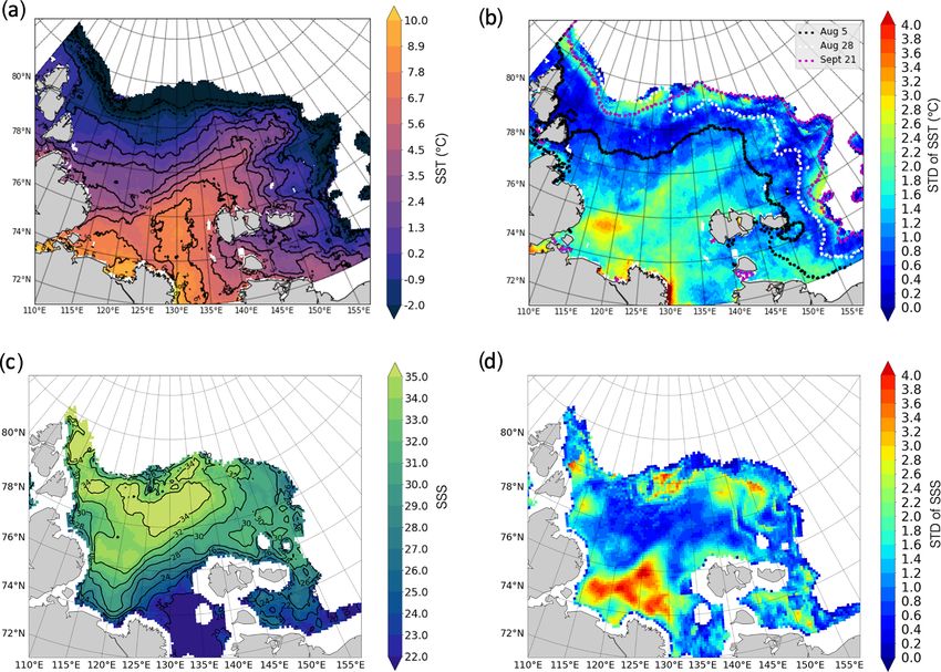
224 A. Tarasenko et al.: Properties of surface water masses in the Laptev Sea
close to the ice edge. Standard oceanographic stations (145 in
total) were conducted with a SeaBird SBE911plus CTD in-
strument equipped with additional sensors. For this study, we
use mainly the CTD measurements of potential temperature
and practical salinity but also the results of oxygen isotope
analysis from the first (surface) bottle samples (Alkire and
Rember, 2019). All CTD data were processed and quality
checked. The cruise data can be found at https://arcticdata.
io/catalog/data, last access: 24 January 2021 (Polyakov and
Rember, 2019) and Ivanov (2019).
The ship was equipped with an underway measurement
system Aqualine Ferrybox, widely known as a thermos-
alinograph (TSG). The instrument had a temperature and a
conductivity (MiniPack CTG, CTD-F) sensors and a CTG
UniLux fluorometer installed; thus, continuous temperature,
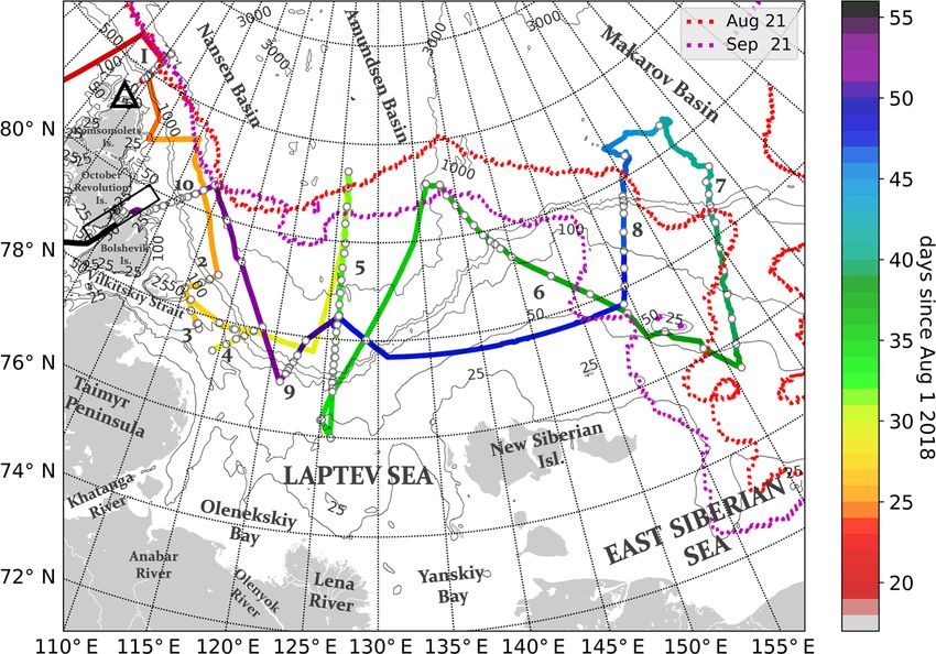
Figure 1. Legs and stations of the ARKTIKA-2018 expedition salinity, and chlorophyll-a estimations were obtained along
overlaid on the bathymetry from ETOPO1 “1 arcmin Global Re- the ship’s trajectory. The inflow is situated at 6.5 m below the
lief Model” (Amante and Eakins, 2009). CTD stations are shown surface (the inflow hole is on the ship’s hull). All data were
with white dots. The color indicates the number of days since 1 Au- processed and filtered for random noise and poor quality
gust 2018. The sea ice edge position is indicated with a dashed red measurements and then compared and calibrated with CTD
line for the beginning (21 August) and with a dashed purple line measurements. When calculating a linear regression between
for the end of the expedition (21 September). The ice edge is based
CTD measurements at 6.5 m depth and TSG measurements,
on the sea ice mask provided in the DMI SST product. Numbers
indicate positions of 10 oceanographic transects discussed below.
we obtain a good correlation for both temperature and salin-
The black triangle in the north of the Komsomolets Island shows ity (correlation coefficient equal to 0.979 and 0.966, respec-
the Arkticheskiy Cape. The Severnaya Zemlya Archipelago con- tively, not shown). The standard error is 0.023◦ for temper-
sists mainly of the Komsomolets, the October Revolution, and the ature and 0.025 for salinity, and the standard deviation (SD)
Bolshevik Islands (with smaller islands not shown here). The black for the difference of measurements (CTD minus TSG) was
box indicates the Shokalskiy Strait between the October Revolution SDtemp = 0.413 ◦ C and SDsal = 0.423. To adjust the contin-
and the Bolshevik Islands. The Yana river estuary (outside the map uous TSG measurements to the more precise CTD measure-
area) is south of Yanskiy Bay ments, we applied the obtained linear regression equation to
TSG data. We only use these adjusted temperature and salin-
ity data.
2.1 In situ measurements during the ARKTIKA-2018 The vertical profiles of the conservative temperature and
expedition practical salinity in the upper layer are presented in Fig. 2. To
investigate if the TSG measurements can be used to study the
Oceanographic measurements during the ARKTIKA-2018 surface layer in a highly stratified Laptev sea, we calculated
expedition on board RV Akademik Tryoshnikov started on a summer mixed layer depth following the de Boyer Mon-
21 August 2018 and ended on 24 September 2018 (Fig. 1). tégut et al. (2004) method based on density and temper-
Oceanographic transects were organized to take into account ature gradient thresholds (Fig. 2a, c). The MLD is found
the requirements of different scientific expeditions on board, at a depth of the first maximum temperature gradient be-
NABOS (Nansen and Amundsen Basin Observational Sys- low a depth of defined (by given threshold) density gradi-
tem) and CATS (Changing Arctic Transpolar System) to ob- ent (see de Boyer Montégut et al. (2004) for details). Us-
serve shallow and continental slope processes. NABOS tran- ing the same approach, we computed MLD with density and
sects were mostly cross-shelf (1, 5, 6–8, 10), and CATS tran- salinity vertical profiles. The threshold chosen for practical
sects were shallower (2–4, 9). Transects 3 and 10 were made density gradient was 0.3 kg m−3 m−1 and 0.2 units per 1 m
in the straits between the Kara and the Laptev seas: transect 3 for conservative temperature and practical salinity gradients.
in the Vilkitskiy Strait southward to the Bolshevik Island, Regarding the MLD calculated from salinity (MLDsal ), most
with depths from 70–200 m opening into the deep central of the measured vertical profiles (75.17 %) had the MLDsal
part of the Laptev Sea (more than 1000 m), and transect 10 below 7 m depth with the median of MLDsal 11.99 m. As
in the narrow and rather shallow (250 m) Shokalskiy Strait for the temperature (MLDtemp ), 81.37 % of the measured
between the Bolshevik and the October Revolution Islands. profiles had the MLD below 7 m depth with a median of
Some measurements were carried out in the MIZ and ice- MLDtemp = 13.50 m. Thus, in most cases the upper 12 m of
covered area (see the sea ice edge positions at the begin- the surface layer was homogeneous, and the CTD and TSG
ning and the end of the cruise in Fig. 1). In this study we measurements can be used for the validation of satellite data.
define MIZ as an area with 0 %–30 % sea ice concentration The median vertical profiles of temperature and salinity in
Ocean Sci., 17, 221–247, 2021 https://doi.org/10.5194/os-17-221-2021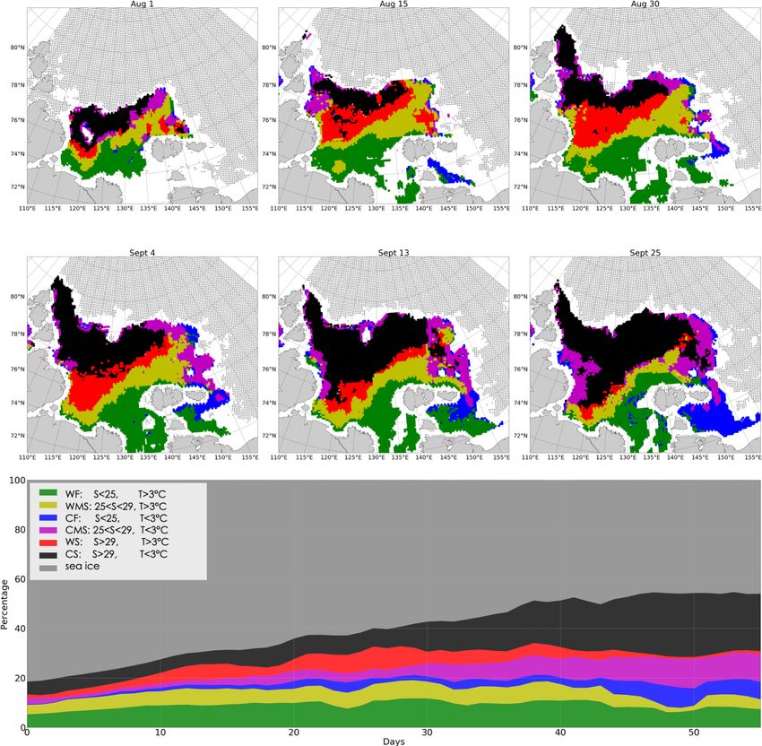
A. Tarasenko et al.: Properties of surface water masses in the Laptev Sea                                                              225

Figure 2. Vertical profiles of conservative temperature (a, b) and practical salinity (c, d) from CTD measurements in the upper ocean layer.
Panels (a) and (c) show all vertical profiles in the upper 50 m, calculated using de Boyer Montégut et al. (2004) method (see details in the
text): red stars indicate the mixed layer depth, colored profiles show the cases when the MLD is below 7 m depth, and gray profiles indicate
when the MLD is above 7 m depth. Panels (b) and (d) show the median vertical profiles in the 5–100 m layer of temperature and salinity,
respectively, where the shaded area shows the associated SD.

the upper 5–100 m are presented in addition to the associ-              2.1.1    River discharge
ated SD in Fig. 2b, d). We observe rather cold (0.5 ◦ C) and
fresh (30.5) water at 5 m, followed by a smooth thermocline             To illustrate the amount and temporal variability of the river
and halocline down to 30 m depth (with a temperature of                 discharge in 2018, we used daily measurements of the Lena
−1.3 ◦ C and salinity of 33.8). Below 30 m the temperature              River discharge from the Arctic Great Rivers Observatory
rises slightly to −1 ◦ C and salinity stays close to 34.5. The          (GRO) dataset (https://arcticgreatrivers.org/data/, last access:
SD of conservative temperature is the largest at the surface            24 January 2021). In Fig. 3 we present a time series of the
(1.55 ◦ C) and smallest at 40 m depth (0.27 ◦ C). The SD of             Lena River discharge from May to November 2018. The river
salinity is also the largest at the surface (1.50) but diminishes       stayed under the ice with a very small discharge up to the
with depth to 0.20 at 100 m. Nevertheless, it is clear that at          end of May. The main peak of the Lena River discharge oc-
the end of a summer season in this region with very different           curred in the beginning of the Arctic summer in June and
water origins, these median profiles are not representative for         corresponds to the snow and ice melting over the river basin
all water masses. Additionally, we did an important number              in Siberia. Over 2 weeks, the discharge changed from 2500
of CTD casts in very shallow areas with depths between 30               to 120 000 m3 s−1 . The second, smaller peak of the river dis-
and 50 m, and thus the calculated averaged (median) vertical            charge occurred at the beginning of August (60 000 m3 s−1 ),
profile is composed of “shallow” and “deep” vertical profiles.          which might be associated with summer precipitation. Dur-
We do not include the very surface measurements above 5 m               ing August 2018 the river discharge decreased from 60 000
because we only had 45 CTD measurements at 2 m depth                    to 40 000 m3 s−1 , and in September it varied very little, stay-
among the 146 possible and taking them into account would               ing close to 40 000 m3 s−1 . A significant diminution of the
bias the median profiles as well.                                       river discharge started in the beginning of October and con-
                                                                        tinued up to the beginning of November. After the beginning
                                                                        of November the river discharge was very weak and close to
                                                                        its minimum values (4500 m3 s−1 ).

https://doi.org/10.5194/os-17-221-2021                                                                   Ocean Sci., 17, 221–247, 2021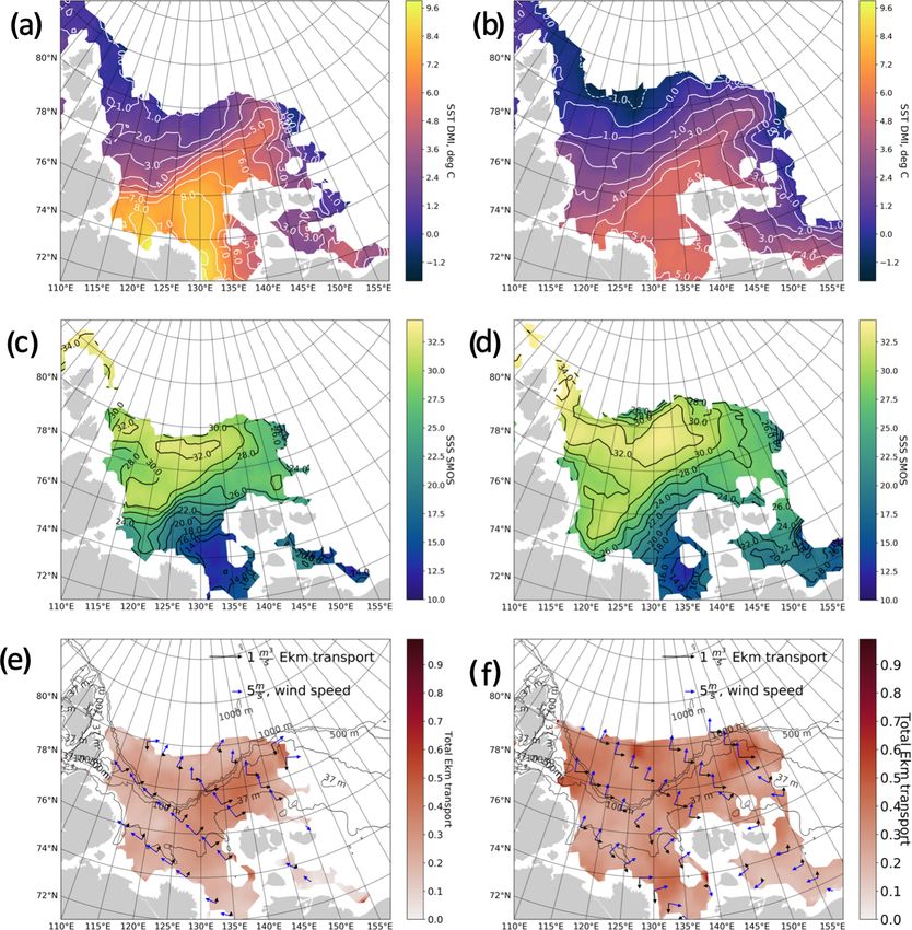
226                                                    A. Tarasenko et al.: Properties of surface water masses in the Laptev Sea

                                                                        nicus Marine service. Daily surface temperatures over the sea
                                                                        and ice are derived on a 5 km spatial grid from several instru-
                                                                        ments: AVHRR, VIIRS for SST, and AMSR2 for sea ice con-
                                                                        centration using optimal interpolation (Høyer et al., 2014).
                                                                           Besides the full coverage over the studied area, the advan-
                                                                        tage of the blended DMI SST product is that it takes into
                                                                        account the ice temperature, and thus the marginal ice zone
Figure 3. The Lena River discharge in 2018. Data taken from the         is better represented and not masked out. The total number
Arctic GRO dataset (https://arcticgreatrivers.org/data/, last access:   of SST measurements ingested over the studied area from
24 January 2021).                                                       1 August to 25 September 2018 varies from 1000 to 2500
                                                                        measurements per pixel.

   The described seasonal dynamics are typical for the Lena             2.2.2   Validation of DMI SST
River and consistent with existing results, e.g., those demon-
strated in Janout et al. (2015). They can be complemented by            The first step of the DMI SST validation was its value-by-
the results of the Papa et al. (2008) study of the large Siberian       value comparison with a colocated in situ dataset (nearest-
rivers using satellite data. Papa et al. (2008) showed that             neighbor DMI SST pixel). For this analysis, we colocated
the maximum of precipitation over the basins of the Lena,               DMI SST with the in situ potential temperature measure-
the Ob, and the Yenisey rivers occurs in July, and the mean             ments in the upper 6.5 m layer: all available CTD measure-
monthly air temperature is at its maximum at that time.                 ments averaged every half a meter above 6.5 m depth and all
                                                                        TSG measurements at 6.5 m depth averaged every 30 min.
2.2     Satellite data                                                  The median depth of the colocated CTD measurements is
                                                                        5.25 m. As for the TSG, the ship was moving with a me-
Satellite data provide information on the surface distribution          dian speed of 8 kn during the cruise, and thus an average of
of geophysical characteristics over the whole study area to-            30 min TSG measurements is an average over approximately
gether with their temporal evolution.                                   7.5 km. Thus, a 30 min TSG average is comparable with one
   All products listed below are considered from 1 August to            DMI SST pixel (10 km). There were 1707 colocated points
25 September 2018 (the last day of ARKTIKA-2018 expe-                   in the analysis.
dition). For consistency, when not specifically indicated, all             Although satellite SST estimates may differ from the in
products are linearly interpolated on a regular grid within the         situ temperature measurements in the upper 6.5 m, we ex-
box 74–85◦ N, 90–170◦ E, with a 0.01◦ step in latitude and              pect an overall consistency between the datasets. Studies car-
0.05◦ in longitude. The spatial resolution of the selected grid         ried out by Castro et al. (2017) devoted to the validation
roughly corresponds to 1 km.                                            of MODIS SST in the MIZ and by Vivier et al. (2016),
                                                                        which described in situ measurements in the iced-covered
2.2.1    Sea surface temperature                                        area, reported that the first 7–10 m layer below the surface
                                                                        was mostly homogeneous. As is shown in Fig. 2, most of
The sea surface temperature (SST)-retrieving instruments                our measurements (more than 75 %) were homogeneous in
with the highest resolution, such as AVHRR (Advanced Very               the upper 12 m (and were done in the ice-free areas). Nev-
High Resolution Radiometer), MODIS (Moderate Resolu-                    ertheless, a diurnal warming and local vertical mixing can
tion Imaging Spectroradiometer), and VIIRS (Visible In-                 affect the vertical temperature distribution in the very sur-
frared Imaging Radiometer Suite), work in near-infrared                 face layer. The SST diurnal amplitude can reach more than
(NIR) and infrared (IR) bands and strongly depend on atmo-              3 K in the Arctic Ocean (Eastwood et al., 2011). To create
spheric conditions (providing measurements only for clear               DMI SST L4 product, only the observations between 21:00
sky without clouds). For lower-resolution microwave instru-             and 07:00 local time are used (Høyer et al., 2014), thus lo-
ments, such as AMSR2 (Advanced Microwave Scanning Ra-                   cal diurnal variations of SST are supposed to be filtered out.
diometer 2), the clouds are transparent, but the SST retrievals         Diurnal variation of temperature might be present in real in
may still be hampered by high wind speed and precipita-                 situ measurements during strong diurnal warming events, but
tion events. As satellite measurements in IR and NIR ranges             no particular observations allowing the investigation of this
are sparse because of the frequent cloudiness over the Arctic           question were done during the cruise.
Ocean, we used a blended product. In this paper we use the                 To illustrate the consistency of SST and in situ temperature
Danish Meteorological Institute Arctic Sea and Ice Surface              datasets, 13 September 2018 was considered, as it was one
Temperature product (hereafter referred to as “DMI SST”).               of the rare days in summer 2018 when the central part of the
DMI SST is a Level 41 daily product provided by the Coper-              Laptev Sea was cloud-free, which is especially important for
    1 “Level 4 product” means that several swath measurements were      DMI SST.
interpolated to achieve a regular resolution in time and space.

Ocean Sci., 17, 221–247, 2021                                                               https://doi.org/10.5194/os-17-221-2021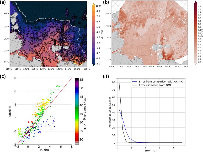
A. Tarasenko et al.: Properties of surface water masses in the Laptev Sea                                                               227

Figure 4. Sea surface temperature validation shown with an example of a DMI SST L4 image for 13 September (a) and the same image
shown with the error estimates (b), a comparison of colocated SST and in situ data (CTD and TSG) in the upper 6.5 m (c), and the distribution
of uncertainty provided by DMI and absolute difference derived from comparison with in situ data (d).

   The DMI SST product for 13 September, presented in                    age 0.3 ◦ C warmer than the 3–6.5 m layer (not shown). The
Fig. 4a, shows a rather complex pattern with a pronounced                largest deviations are observed when the ship is in the MIZ or
gradient associated with warm river water in the central part            a more compact sea ice, so they might be associated with ei-
of the Laptev Sea. The uncertainty in SST estimates provided             ther imperfect sea ice flagging of some stages of sea ice in the
by DMI is shown in Fig. 4b, d. The percentage of occur-                  DMI SST product or a noise introduced after re-interpolation
rence is computed for 0.5 ◦ C temperatures classes starting at           of data on a regular grid. This noise, together with the differ-
0 ◦ C (Fig. 4d). The highest uncertainty (up to 2.5 ◦ C) was ob-         ent sampling of in situ potential temperature measurements
served over some open-sea areas that were partially cloudy               and the DMI SST product, lead to a distribution of the abso-
but was mostly associated with the sea ice due to its hetero-            lute differences between in situ and DMI SST that is slightly
geneity (Fig. 4b). Over most of the southern and the central             wider than the one of uncertainties provided in the DMI SST
part of the ice-free Laptev and the East Siberian seas, the un-          product (Fig. 4d). Nevertheless, this comparison should be
certainty is below 0.5 ◦ C, and over the eastern part it is below        taken only as indicative of a reasonable order of magnitude of
1 ◦ C.                                                                   the uncertainties given the limited number of in situ measure-
   Comparison of the DMI SST and in situ surface-layer tem-              ments for each uncertainty range. After removing the bias,
perature (Fig. 4, c) shows a good agreement that is almost in-           the correlation coefficient is 0.89 and the rms difference is
dependent of area and time during the ARKTIKA-2018 ex-                   0.77 ◦ C. Overall, DMI SST agrees rather well with in situ
pedition. The bias (difference between mean DMI and mean                 data, and it captures a small-scale spatial variability of the
in situ surface temperature data) is 0.19 ◦ C. This excess av-           SST in the ice-free areas (Fig. 4a) well above SST uncertain-
erage DMI SST seems to be possible, based on CTD mea-                    ties, and thus we use this product for the following analysis
surements, indicating that the 0–3 m water layer is on aver-             of SST time series.

https://doi.org/10.5194/os-17-221-2021                                                                    Ocean Sci., 17, 221–247, 2021
228                                                A. Tarasenko et al.: Properties of surface water masses in the Laptev Sea

2.2.3   Sea surface salinity                                       pling over the Arctic Ocean and to decrease the uncertainty
                                                                   with temporal averaging. In order to eliminate the SSS at
Soil Moisture and Ocean Salinity (SMOS) is the first satel-        very low and high wind speeds because of higher uncertain-
lite mission carrying an L-band (1.41 GHz) interferometric         ties, SMOS ESA L2 SSS was considered only if the associ-
microwave radiometer, from which measurements are used             ated ECMWF (European Centre for Medium-Range Weather
to retrieve the sea surface salinity (SSS) in the top centimeter   Forecasts) wind speed was between 3 and 12 m s−1 . SMOS
of the water. With the recent processing, the standard devia-      ESA L2 SSS measurements were also weighted relative to
tion of the differences between 18 d SMOS SSS and 100 km           the uncertainty of the SSS measurement (as in Yin et al.,
averaged TSG surface salinity measurements is 0.20 in the          2013, Eq. A7). This uncertainty was derived from informa-
open ocean between 45◦ N and 45◦ S (Boutin et al., 2018).          tion provided with the SMOS L2 products, the SSS “theo-
However, the precision degrades in cold water as the sen-          retical error”, derived from the uncertainty of all the param-
sitivity of L-band radiometer signal to SSS decreases when         eters used for retrieving SMOS SSS, multiplied by the nor-
SST decreases, even though this effect on temporally aver-         malized χ 2 cost function of the SSS retrieval. Dinnat et al.
aged maps is partly compensated for by the increased num-          (2019) showed that the Klein and Swift (1977) dielectric
ber of satellite measurements at high latitude (Supply et al.,     constant model was inaccurate at low SST. In order to mit-
2020). The possibility of using SSS estimates in cold regions      igate this effect, a SST-dependent correction derived from
derived from L-Band radiometry has been recently demon-            Fig. 16 of Dinnat et al. (2019) (blue-circle line) was applied:
strated by several working groups (Tang et al., 2018; Grod-        SSSSMOS-“A” = SSSSMOS−ESA−L2 −(−5·10−4 ·SST3ECMWF +
sky et al., 2018; Olmedo et al., 2018). However, existing L32      0.02 · SST2ECMWF − 0.23 · SSTECMWF + 0.69).
SSS products, e.g., SMAP CAP/JPL (Soil Moisture Active                Finally, a criterion for a SMOS-retrieved pseudo-dielectric
Passive satellite, a product created using the Combined Ac-        constant (ACARD parameter, defined in Waldteufel et al.,
tive Passive algorithm by Jet Propulsion Laboratory) SSS, or       2004), was applied to discard SMOS measurements affected
SMOS BEC (Barcelona Expert Center) SSS, are spatially av-          by sea ice (discarded when ACARD < 45). The uncertainty
eraged from 60 km to more than 100 km.                             of SMOS SSS “A” was derived from the propagation of the
   SMAP REMSS (Remote Sensing Systems) SSS L3 v3                   uncertainty on individual SMOS ESA L2 SSS pixel during
provides a 40 km resolution version but does not provide a         7 d. The uncertainty strongly increases in the vicinity of sea
sufficient coverage in the Laptev Sea. The methodology de-         ice (Fig. 5b). For this reason, in the following study, above
veloped in this study to retrieve SMOS SSS aims to maintain        75◦ N, all pixels with an SSS weekly uncertainty larger than
SMOS original spatial resolution and retrieve SSS as close         0.8 were not considered. South of 75◦ N, a higher threshold
as possible to the ice edge.                                       was used (1.5) allowing us to maintain some measurements
   A new product, hereafter SMOS SSS “A” (“A” for the Arc-         closer to fresh river water from the Lena and the Khatanga
tic Ocean) L3, investigated in this study was computed using       rivers near the coast. In this area, the χ 2 may increase due to
SMOS L23 SSS from the ESA (European Space Agency) last             the strong heterogeneity of SSS within SMOS multi-angular
processing (v662, Arias and Laboratories, 2017), (Fig. 5a).        brightness temperatures footprints, and the number of mea-
SMOS L2 SSS are available on the ESA SMOS Online Dis-              surements is low due to the presence of the coast and islands
semination website. SMOS SSS are representative of SSS in-         even without sea ice. The theoretical uncertainty of SMOS
tegrated over about 50×50 km2 given the footprint of SMOS          SSS “A” field is below 0.5 in the center of the Laptev Sea
radiometric measurements involved in the SSS retrievals.           and up to 2 and higher close to the coastline and MIZ.
The SMOS ESA L2 SSS products are oversampled over an
Icosahedral Snyder Equal Area (ISEA) grid at 15 km resolu-         2.2.4   Validation of SMOS “A” SSS
tion. The oversampling on a 15 km grid is possible owing to
the image reconstruction of the SMOS interferometric data,         In this section, we compared the SMOS SSS “A” relative to
but in this processing we do not make any spatial average for      in situ measurements. Figure 5 presents the SMOS SSS “A”
SSS fields.                                                        on 13 September 2018, the same day as the DMI SST in
   SMOS “A” SSS was obtained as described below. The 7 d           Fig. 4. We colocated SMOS SSS “A” and in situ measure-
running means were computed for each day and each pixel            ments of salinity in the upper 6.5 m layer in the following
of the ISEA grid, using a temporal Gaussian weighting func-        manner: the averaging of the TSG salinity was done over a
tion with a standard deviation of 3 d. The full width of SMOS      1 h period (equal to ∼ 15 km distance, contrary to DMI SST
ascending and descending orbits swaths was considered in           validation) in order to be closer to SMOS SSS “A” spatial
order to take advantage of better temporal and spatial sam-        resolution. We used 985 colocated points.
                                                                      Comparison between the in situ practical salinity and
   2 “Level 3” means a product resampled at a uniform temporal–    SMOS SSS “A” shows a very good agreement that has not
spatial grid, different from a swath grid.                         yet been demonstrated before by any other salinity prod-
   3 “Level 2” product means that a geophysical parameter, e.g.,   uct in the Laptev Sea. The mean difference is 2.06, SMOS
SSS, was computed at the swath grid.                               SSS being lower than in situ surface salinity. This underes-

Ocean Sci., 17, 221–247, 2021                                                          https://doi.org/10.5194/os-17-221-2021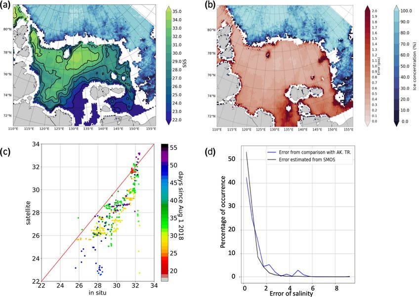
A. Tarasenko et al.: Properties of surface water masses in the Laptev Sea                                                                 229

Figure 5. Sea surface salinity validation shown with an example of SMOS SSS “A” for 13 September 2018 (a) and associated uncertainties
(b), a scatterplot of colocated SSS and in situ data in the upper 6.5 m (c), and statistical distribution of provided SMOS L2 uncertainties and
measured absolute difference from comparison with in situ data (d). Sea ice concentration from AMSR2 is indicated with blue shading on
the upper panels

timate could be related to the presence of land in the very               SSS “A” uncertainties estimated from the retrieval process
wide SMOS field of view as observed at lower latitudes by                 and the distribution of error obtained from comparison with
Kolodziejczyk et al. (2016), and this difference appears to be,           in situ salinity measurements. The uncertainties are in 85 %
at first order, systematic (Fig. 5c). In what follows, we sub-            of cases less than 1.2, which is relatively small compared to
tract this mean difference from the entire SMOS SSS dataset.              spatial gradients shown on Fig. 5a. These results allow us to
The correlation coefficient is then 0.86, with a rms difference           use the SMOS SSS “A” error with confidence for this analy-
equal to 0.86. The standard deviation of SMOS SSS with re-                sis. Using error filtering, the points too close to the ice edge
spect to in situ SSS does not vary with the depth of the in               were excluded.
situ salinity measurements above 6.5 m, either because in situ
salinity was homogeneous vertically or because comparisons                2.2.5   Sea ice concentration and ice masks
were too noisy to detect these small variations (not shown).
Although SMOS SSS “A” shows a good agreement most of                      Sea ice masks were obtained from AMSR2 sea ice concentra-
the time, some larger uncertainties occur close to the sea ice            tions products provided by the University of Bremen (Spreen
margin or when pixels are contaminated by small ice pattern               et al., 2008): they are weather independent and thus continu-
not detected by AMSR2 sea ice concentration algorithm (as                 ous for the whole period. The highest available spatial res-
at 80◦ N, 125◦ E in Fig. 5a).                                             olution is 3.125 km. The AMSR2 ice masks were used in
   Comparison between SMOS uncertainties and error based                  addition to the masks provided with every satellite product
on comparison with in situ salinity measurements is pre-                  discussed: DMI SST, SMOS SSS “A”, ASCAT (Advanced
sented in Fig. 5d. The percentage of occurrence is computed               SCATterometer) winds L3 (see its description below). A con-
in salinity classes with a size of 0.5 that starts at 0. It shows         tinuous erroneous presence of ice along the Siberian coast
a rather good agreement between the distribution of SMOS                  was observed and had to be filtered: images in the optical
                                                                          band and the ice charts from the Arctic and Antarctic Re-

https://doi.org/10.5194/os-17-221-2021                                                                     Ocean Sci., 17, 221–247, 2021
230                                                A. Tarasenko et al.: Properties of surface water masses in the Laptev Sea

search Institute (AARI) were used as a reference (can be           3     Results
found at http://www.aari.ru/odata/_d0004.php, last access:
24 January 2021). As detailed above, an additional filtering       3.1    Overview of SST and SSS in the Laptev and East
was applied to SMOS SSS “A”, as the L-Band measurements                   Siberian seas in August–September 2018
are sensitive to ice thicknesses less than 50 cm in contrast
with the AMSR2 measurements.                                       The mean SST during the 2 summer months is 2.18 ◦ C in the
   The sea ice opening starts relatively late in the Laptev Sea:   Laptev Sea (between the Severnaya Zemlya Archipelago and
a coastal polynya appeared in the southern central part of         the new Siberian islands), and 1.13 ◦ C in the part of the East-
the Laptev Sea at the beginning of June 2018, and by the           Siberian Sea investigated (Fig. 6). The highest temperatures
beginning of August the sea was only ice-free south of 79◦ N.      (above 6 ◦ C, up to 9 ◦ C) were observed close to the Lena
The Laptev Sea was completely covered by the beginning of          River delta in Yanskiy Bay and in Olenekskiy Bay in front
November 2018. For this study, we define the sea ice edge          of the Khatanga River. A warm water pool associated with
with the position of 1 % sea ice concentration and MIZ as          the river plume between 125 and 135◦ E progressively prop-
0 %–30 %.                                                          agates northeastward and warms up this part of the sea: 0 ◦ C
                                                                   isotherm at 140◦ E meridian is situated 100 km northward
2.2.6    Wind speed                                                compared to its position at 120◦ E. The studied part of west-
                                                                   ern East Siberian Sea was not completely ice-free in August–
To investigate the wind speed pattern, we use ASCAT scat-          September 2018. Negative temperatures are observed near
terometer daily C-2015 L3 data produced by Remote Sensing          the ice edge at a distance of 50–100 km of the ice edge al-
Systems. Data are available at http://www.remss.com.               most everywhere, except for a small area at 80◦ N, 160◦ E,
                                                                   where warm river water meets the sea ice with no open wa-
2.3     Reanalysis data
                                                                   ter with negative temperatures. The strongest gradients are
Reanalysis data are used to include some additional parame-        observed along the sea ice edge and the river water plume
ters not available from satellite and in situ data. Atmospheric    (up to 0.05 ◦ C km−1 ). Standard deviation of SST in Fig. 6 is
forcing fields, i.e., sea level pressure (SLP) and air tempera-    the largest in Olenekskiy Bay (over 2.5 ◦ C), along the coast-
ture, are obtained from the ERA5 reanalysis (Bertino et al.,       line close to the Khatanga estuary (2.5–3 ◦ C), the Lena River
2008). The latest reanalysis of ERA5 still has a relatively        delta (about 4 ◦ C), and in marginal ice zone (mostly over
crude spatial grid of 0.5◦ for the SLP and 0.25◦ for air tem-      1.5 ◦ C). The remarkable variation of SST in the central part
perature.                                                          of the Laptev Sea should be associated with the thermal front
                                                                   (largest SST gradients) displacement.
2.4     Ekman transport                                               The averaged SSS is 28.75 (with uncertainty of 0.10) in
                                                                   the Laptev Sea and 27.74 (with uncertainty of 0.20) in the
To investigate the role of the wind forcing, we compute mean       western East Siberian Sea (Fig. 6). The spatial distribution of
monthly wind fields and the Ekman transport for August and         mean salinity for August–September 2018 shows the fresh-
September 2018. Horizontal Ekman transport (m2 s−1 ) is cal-       est water (salinity below 20) within the river plume north-
culated as follows:                                                east of the Lena River delta and within the southern part of
         τv                                                        the East Siberian Sea. Water with salinity below 28 reaches
uekm =                                                             the sea ice edge in the northeastern Laptev Sea. Additional
       ρw · f
           τu                                                      fresher water from the Kara Sea enters via the Vilkitskiy
vekm = −        ,                                           (1)    and Shokalskiy straits in the west (salinity of 28–30) and
         ρw · f                                                    is also observed along the sea ice edge, where it could be
where uekm and vekm are horizontal components of the Ek-           associated with ice melting. The most saline water (salinity
man transport; τ is wind stress, calculated from ASCAT             above 34) is located in the central part of the Laptev Sea near
winds (uwind , vwind ) using ERA5 air density ρair : τu = CD ·     78–80◦ N, 120–140◦ E and in the northwest along the Sev-
|uwind | · uwind · ρair (and similarly for τv ); ρw is a surface   ernaya Zemlya Archipelago. As also observed in SST, SSS
density, calculated from SST and SSS with TEOS-10 (Mc-             in the Olenekskiy Bay is highly variable, which can be ex-
Dougall et al., 2009); CD is surface drag coefficient, cal-        plained by the variation of the freshwater discharge during
culated from wind speed according to Foreman and Emeis             the 2 months. Nevertheless, large SSS variability is also ob-
(2010); and f is the Coriolis parameter.                           served all along the sea ice edge: at 78–80◦ N in the north
                                                                   and northwest and at the boundary between the Laptev and
                                                                   East Siberian seas. This large variability can be explained in
                                                                   two ways: physical (haline fronts related to sea ice melting)
                                                                   and instrumental (remaining ice contaminated pixels, lower
                                                                   sensitivity of L band in cold water). At 78–80◦ N, 125◦ E,
                                                                   free-floating patches of broken ice detached from compact

Ocean Sci., 17, 221–247, 2021                                                          https://doi.org/10.5194/os-17-221-2021
A. Tarasenko et al.: Properties of surface water masses in the Laptev Sea 231
Figure 6. Mean DMI SST (a) with its SD (b) and mean SMOS SSS (c) with its SD (d) for August–September 2018. The dotted lines
in (b) show the position of the sea ice edge at different moments of time before and during the ARKTIKA-2018 cruise.
sea ice edge are observed during several weeks in August– lowest values presented in Fig. 7, −1.7 to 2.5 ◦ C. The sur-
September 2018. Random pieces of broken sea ice are not face water observed in the upper 50 m is in general less saline
always recognized by ice-mask filters, and thus they can ar- (salinity below 34), but we can clearly observe two separate
tificially increase SSS variability. At the same time, this is branches with negative and positive temperatures. The two
the area where river water encounters sea ice, which induces upper-layer branches are (1) warmer ([−1; 6] ◦ C) and low-
natural variability. saline (below 34) surface water of the ice-free Laptev Sea
and (2) colder ([−2; 0] ◦ C) and low-saline waters of the ice-
3.2 Observed surface water masses of the Laptev Sea covered East Siberian Sea. The latter corresponds to the mea-
and their transformation surements from the transects 7 and 8 eastward of 150◦ E.
It should be remembered that a T –S diagram based only
on CTD measurements does not provide an instantaneous
To generalize our understanding of vertical structure of the
view on the ocean state but is a collection of conditions en-
studied area, we use the classical T –S analysis, first based
countered in different regions at different times (from the end
on CTD measurements. Figure 7 shows the temperature–
of August to the end of September 2018). During the sum-
salinity distributions in the upper 200 m, colored as a func-
mer months, the surface water of the Arctic Ocean quickly
tion of depth. The most prominent feature on the diagram is
evolves, and the synoptic satellite data provide an additional
the transformed Atlantic Water mass with salinity close to
information to the point-wise in situ measurements.
34.5–35, temperatures from −0.5 to 2.5 ◦ C lying at a depth
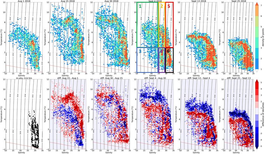
Using DMI SST and SMOS SSS weekly estimates, we
of 100–200 m. The water mass overlying the Atlantic Water
plotted T –S diagrams similar to the one in Fig. 7, but only for
(between 50 and 100 m depth) is the lower halocline water,
surface satellite measurements for several reference days: 1,
described by Dmitrenko et al. (2012) as having salinity in a
15, 30 August, 4, 13, and 30 September 2018 (Fig. 8). On the
range 33–34.5, and negative temperatures starting from the
https://doi.org/10.5194/os-17-221-2021 Ocean Sci., 17, 221–247, 2021232 A. Tarasenko et al.: Properties of surface water masses in the Laptev Sea
temperature and salinity ranges of variation of each class are
also well above the T and S uncertainties.
The main surface water masses are warm and fresh (WF)
river water and cold and saline (CS) open sea water. All other
water masses show either different stages of transformation
of these two water masses or are advected from other regions.
It should be noted that satellite-derived data have a larger
range of temperature and salinity than the near-surface (up-
per 6.5 m) in situ measurements, which enables this detailed
classification. The locations of the different water masses for
specific days are shown in Fig. 9 together with the percent-
age distribution of water masses (the whole studied area is
100 %, and sea ice occupies some part of it).
On 1 August, the sea ice still covers more than 80 % of the
studied area and extends on average to 78◦ N in the Laptev
Sea, while the East Siberian Sea is almost completely cov-
ered by ice. WF river water is easily observable in the south-
ern parts between 74 and 76◦ N. It occupies almost the same
amount of surface as the CS, the rest of the open area is occu-
pied by a transformed river water (warm and medium salin-
ity, WMS; cold and medium salinity, CMS), which already
formed a recognizable river plume front: its signature is con-
tinuous from 115 to 150◦ E up to the northern position of sea
Figure 7. T –S diagram based on the CTD data in the upper 250 m, ice edge.
color coded by depth. The red line shows the freezing line. During the next 2 weeks the ice cover retreats, and a CF
mass appears in the southwestern East Siberian Sea. The
amount of this water increased progressively in this area
lower row, we present all in situ measurements in the upper during the remaining period. We suggest that this water
6.5 m and the differences between satellite-derived sea sur- mass represents the river water trapped under the ice and
face temperature and salinity for the selected day. The range then exposed (see results of geochemical analysis below in
of variation in SSS and SST values covered by the satellite Sect. 3.3.4).
measurements (first row of Fig. 8) is an order of magnitude On the 15 August, a water mass CMS also appears close
wider than the one covered by in situ measurements (Fig. 8, to the Vilkitskiy Strait. It is less pronounced by the end of
first column, bottom row). The difference in T –S diagrams August, but a thin stream of cooled and transformed river
covered by each type of measurement cannot be explained water from the Kara Sea extends along the Taimyr peninsula
by the errors of satellite measurements (rms difference with in September. The Lena River water mixing and cooling also
respect to in situ measurements of 0.77 ◦ C and 0.8 in temper- happens close to the sea ice edge in the northeastern Kara
ature and salinity, respectively) or by the uncertainties asso- Sea. As a whole, the surface occupied by this water mass is
ciated with each satellite product (Figs. 4b and 5b). It primar- steadily growing during the observed period to reach nearly
ily reflects the much more extensive spatiotemporal monitor- 10 % of the surface by the end of September. We suggest that
ing of different water masses by satellite measurements, e.g., water mass CMS is a transformed version of water mass CF.
the in situ measurements miss the southern Laptev sea, close The end of August is warmer, as seen in Fig. 9; saline wa-
to the origin of the riverine water. The DMI SST increases ter with temperatures above 3 ◦ C (water mass WS) occupies
only up to the end of August with the maximum tempera- the central and the western part of the Laptev Sea (almost
tures from 8 to 11.5 ◦ C in some cases and then decreases to 10 % of the studied area). This water mass disappears by the
4.5 ◦ C by the end of September. The temperature changes by end of September with the seasonal decrease of temperature.
0.5–1 ◦ C per week (while increasing and decreasing). By 13 September, the SST and SSS variability diminishes.
Based on the Fig. 8 visual analysis, we propose identify- The water mass CF in the northeastern Laptev Sea, consist-
ing 6 surface water masses in the Laptev and East Siberian ing of cold fresh water, becomes saltier (and transforms into
seas (Table 1) to follow the transformation of surface wa- the water mass CMS). The freshwater cools south of the
ters during 2 summer months (Fig. 9). The number and the New Siberian islands and by September 25 occupies all the
limits of water masses were arbitrarily chosen based on the ice-free area. The river plume signature shifts to the New
temperature–salinity scatterplot for 4 September 2018, as Siberian islands as well (Fig. 9). Cold and saline water domi-
this day allows us to separate the cores of surface waters into nates the surface of the Laptev Sea. Finally, by 25 September,
groups in the best way based on the density of points. The the T –S diagram shows that most of the SSS and SST points
Ocean Sci., 17, 221–247, 2021 https://doi.org/10.5194/os-17-221-2021A. Tarasenko et al.: Properties of surface water masses in the Laptev Sea 233
lay between 25 and 35 and −1 and 4 ◦ C, respectively, with a discharge in the first days of September (Fig. 3) introduced
main core within a salinity range 25–35 and temperature be- an additional portion of freshwater that reached 78◦ N several
tween −1 to 1 ◦ C and a second core within the salinity range weeks later.
22.5–30 and temperature of 3–4 ◦ C. The Laptev and the East
Siberian seas then start to refreeze the most rapidly in the 3.3.2 Water from the Kara Sea
areas with cold and fresh river water.
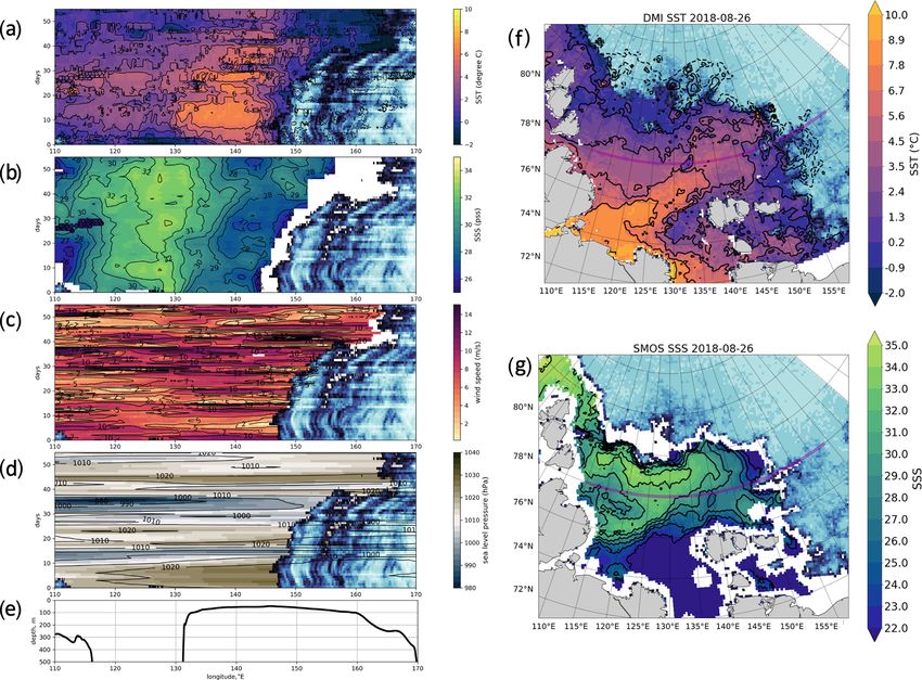
The zonal transect allows us to see not only the Lena River
3.3 Freshwater variability in the Laptev Sea plume but also the Kara water intrusions in the west. The se-
lected zonal transect at 78◦ N is partly lying in the Vilkitskiy
To evaluate the distribution of freshwater input in the Laptev Strait connecting the Kara and the Laptev seas. Being a reser-
Sea in August–September 2018, we consider zonal and voir for two other great Siberian Rivers, the Ob and the Yeni-
meridional transects along 78◦ N, 126◦ E and plot the tem- sei, the Kara Sea has a low salinity compared to the central
poral evolution of DMI SST, SMOS SSS “A”, wind speed, Arctic Basin (Janout et al., 2015). In the absence of signifi-
and SLP in Hovmöller diagrams. The freshwater can be de- cant river sources on the Severnaya Zemlya Archipelago, we
fined by comparison to the saline “marine water” (typically considered that the freshwater input close to the Vilkitskiy
34.80, as in Aagaard and Carmack, 1989, or 34.92, as in and the Shokalsky straits arrived from the Kara Sea.
Bauch and Cherniavskaia, 2018). As zero-salinity river wa- We observe the freshwater arriving from the Kara Sea at
ter quickly mixes with a saltier marine water, in reality the 110–115◦ E with typical values of 25–28 during the first 20 d
“freshwater” is more “brackish” than “fresh”. Nevertheless, of August and at the end of September (Fig. 10b). It is note-
assuming a river plume front at the 29 isohaline for simplic- worthy that the SST fields do not indicate the presence of
ity, the “freshwater” corresponds to all water masses with the these intrusions so clearly. This suggests that fresh and warm
salinity lower than 29, as we mentioned in Sect. 3.2. water of the Ob and Yenisei rivers arriving into the Laptev
Sea have already lost a significant part of their heat content
3.3.1 Water from the Lena River plume to the atmosphere but that the freshwater layer is not com-
pletely mixed with the surrounding sea environment.
The zonal transect helps to investigate the mean stream po- In Fig. 11, the CTD data justify that the amount of fresh-
sition of the river plume away from the coast, in the cen- water arriving from the Kara Sea through the Vilkitskiy Strait
tral part of the Laptev Sea with more complex topography is significantly greater than freshwater arriving via the nar-
(Fig. 10). This virtual transect does not correspond to any row and rather shallow (250 m) Shokalskiy Strait between
real CTD transect, apart from some TSG profiles following the Bolshevik and the October Revolution islands or north
the ship’s route (see the position of virtual transect on the of the Severnaya Zemlya Archipelago at the traverse near
SST and SSS maps in Fig. 10f–g). In the western part (up to the Arkticheskiy Cape across the continental slope. The tem-
130 ◦ E), the transect is located roughly above the continen- perature of the surface layer increases between 0 and 3.5 ◦ C
tal slope and then over the shelf (Fig. 10e). The river water from north to south. Salinity transects indicate freshwater
displacement roughly follows that of sea ice edge in the east with salinity above 29 only in the Shokalskiy and the Vilkit-
and is bounded by the shelf break in the west. Overall, tem- skiy straits, which suggests very little advection of the Kara-
peratures are higher in August than in September: a warm origin freshwater via the north. From the buoyancy cross sec-
pool with SST over 6 ◦ C is observed during the first 30 d at tions, we find that the strongest stratification is at 5–20 m
78◦ N, 130–147◦ E, with the highest temperatures on 26 Au- depth, which corresponds to the 1024–1025 kg m−3 isopy-
gust. These coordinates define the position of the river plume cnals depths. This result argues against a definition of fresh-
at 78◦ N latitude, as can be clearly seen in the salinity values water content by the 1027.35 kg m−3 isopycnal of Polyakov
varying in a range of 27–30. Relatively strong daily winds et al. (2008), as the surface salinity and temperature in the
(10–12 m s−1 ) observed during the first 10 d of September Siberian shelf seas are lower than in other regions.
were associated with a series of cyclones, which strongly
impacted the surface layer: the median temperature over the 3.3.3 Meridional transect
zonal transect decreased from 3 ◦ C to almost 0 ◦ C, and salin-
ity increased by 1. As the amount of incoming solar radiation The meridional transect along 126◦ E (Fig. 12) partly corre-
diminishes in September, the maximum SST values did not sponds to the standard oceanographic transect 5 carried out
exceed 3 ◦ C anymore. Nevertheless, at the end of September, during ARKTIKA-2018 expedition on 1–4 September 2018
a new freshwater patch was observed at 140◦ E (less visible (Fig. 13). This transect helps to understand the northward
in SST field) indicating that the “upstream” surface mixed propagation of the river plume and to evaluate the fresh-
layer (in the southern part of the Laptev Sea) contained a water content using in situ data. The highest SST observed
sufficient amount of freshwater to restore its previous state along 126◦ E longitude is 8 ◦ C in August. Please note that
after a mixing event induced by the wind. Another possible a small cold temperature intrusion on days 22–26 probably
explanation is that a small peak observed in the Lena River corresponds to an error in DMI SST product due to a cyclone
https://doi.org/10.5194/os-17-221-2021 Ocean Sci., 17, 221–247, 2021You can also read