Vertical distribution of chlorophyll in dynamically distinct regions of the southern Bay of Bengal - Biogeosciences
←
→
Page content transcription
If your browser does not render page correctly, please read the page content below
Biogeosciences, 16, 1447–1468, 2019
https://doi.org/10.5194/bg-16-1447-2019
© Author(s) 2019. This work is distributed under
the Creative Commons Attribution 4.0 License.

Vertical distribution of chlorophyll in dynamically distinct
regions of the southern Bay of Bengal
Venugopal Thushara1 , Puthenveettil Narayana Menon Vinayachandran1 , Adrian J. Matthews2 ,
Benjamin G. M. Webber3 , and Bastien Y. Queste3
1 Centre for Atmospheric and Oceanic Sciences, Indian Institute of Science, Bangalore, India
2 Centre for Ocean and Atmospheric Sciences, School of Environmental Sciences and School of Mathematics,
University of East Anglia, Norwich, UK
3 Centre for Ocean and Atmospheric Sciences, School of Environmental Sciences, University of East Anglia, Norwich, UK

Correspondence: Puthenveettil Narayana Menon Vinayachandran (vinay@iisc.ac.in)

Received: 22 June 2018 – Discussion started: 12 July 2018
Revised: 7 February 2019 – Accepted: 22 February 2019 – Published: 9 April 2019

Abstract. The Bay of Bengal (BoB) generally exhibits sur-           chlorophyll distribution in the southern BoB. Stabilizing sur-
face oligotrophy due to nutrient limitation induced by strong       face freshening events and barrier-layer formation often in-
salinity stratification. Nevertheless, there are hotspots of high   hibited the generation of surface chlorophyll. The pathway
chlorophyll in the BoB where the monsoonal forcings are             of the SMC intrusion was marked by a distinct band of
strong enough to break the stratification; one such region          chlorophyll, indicating the advective effect of biologically
is the southern BoB, east of Sri Lanka. A recent field pro-         rich Arabian Sea waters. The region of the monsoon current
gramme conducted during the summer monsoon of 2016,                 exhibited the strongest DCM as well as the highest column-
as a part of the Bay of Bengal Boundary Layer Experi-               integrated chlorophyll. Observations suggest that the persis-
ment (BoBBLE), provides a unique high-resolution dataset            tence of DCM in the southern BoB is promoted by surface
of the vertical distribution of chlorophyll in the southern         oligotrophy and shallow mixed layers. Results from a cou-
BoB using ocean gliders along with shipboard conductivity–          pled physical–ecosystem model substantiate the dominant
temperature–depth (CTD) measurements. Observations were             role of mixed layer processes associated with the monsoon
carried out for a duration of 12–20 days, covering the dy-          in controlling the nutrient distribution and biological produc-
namically active regions of the Sri Lanka Dome (SLD) and            tivity in the southern BoB. The present study provides new
the Southwest Monsoon Current (SMC). Mixing and up-                 insights into the vertical distribution of chlorophyll in the
welling induced by the monsoonal wind forcing enhanced              BoB, emphasizing the need for extensive in situ sampling
surface chlorophyll concentrations (0.3–0.7 mg m−3 ). Promi-        and ecosystem model-based efforts for a better understand-
nent deep chlorophyll maxima (DCM; 0.3–1.2 mg m−3 ) ex-             ing of the biophysical interactions and the potential climatic
isted at intermediate depths (20–50 m), signifying the con-         feedbacks.
tribution of subsurface productivity to the biological carbon
cycling in the BoB. The shape of chlorophyll profiles var-
ied in different dynamical regimes; upwelling was associ-
ated with sharp and intense DCM, whereas mixing resulted            1   Introduction
in a diffuse and weaker DCM. Within the SLD, open-ocean
Ekman suction favoured a substantial increase in chloro-            The Bay of Bengal (BoB) is fascinating, with its unique
phyll. Farther east, where the thermocline was deeper, en-          upper-ocean features strongly linked to the Indian Summer
hanced surface chlorophyll was associated with intermittent         Monsoon (ISM) variability (Gadgil et al., 1984; Vecchi and
mixing events. Remote forcing by the westward propagat-             Harrison, 2002; Shankar et al., 2007). The upper layer of
ing Rossby waves influenced the upper-ocean dynamics and            the BoB, especially the northern BoB, is highly stable, ow-
                                                                    ing to strong near-surface salinity stratification in the pres-

Published by Copernicus Publications on behalf of the European Geosciences Union.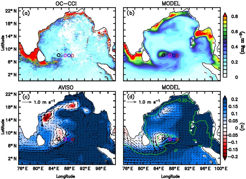
1448                                                        V. Thushara et al.: Chlorophyll distribution in the southern BoB

ence of abundant freshwater influx from precipitation and          Shankar et al., 2002; Lee et al., 2016; Wijesekera et al.,
rivers. The low salinity cap in the surface layers of the BoB      2016b). Unlike the northern BoB, salinity stratification is rel-
leads to the formation of a shallow mixed layer and a bar-         atively weak in the south, resulting in a deeper mixed layer.
rier layer beneath (Vinayachandran et al., 2002; Wijesekera        Prominent chlorophyll blooms are observed in the coastal
et al., 2016a), controlling air–sea interactions and the upper-    and open-ocean regions of the southern BoB, closely linked
ocean heat budget (Shenoi et al., 2002). In addition, mon-         to monsoon circulation (Vinayachandran, 2009). The region
soonal winds are relatively weak over the BoB, leading to a        off the southern coast of Sri Lanka is characterized by high
sluggish upper ocean, where vertical overturning and mix-          chlorophyll levels in summer, triggered by the coastal up-
ing processes are weak (Shetye et al., 1991; Madhupratap           welling of nutrients (Vinayachandran et al., 2004). Cyclonic
et al., 1996; Kumar et al., 2002; McCreary et al., 2009; Wig-      wind stress curl east of Sri Lanka during the summer mon-
gert et al., 2009). This dynamical set-up imparts strong nu-       soon leads to the formation of the Sri Lanka Dome (SLD;
trient limitation on phytoplankton growth, leading to weak         Vinayachandran and Yamagata, 1998), where open-ocean
biological productivity in the BoB (Gomes et al., 2000; Ku-        Ekman suction of nutrients triggers chlorophyll bloom gen-
mar et al., 2002; Madhupratap et al., 2003). Compared to           eration (Vinayachandran et al., 2004). The Southwest Mon-
the highly productive Arabian Sea, chlorophyll distribution        soon Current (SMC) intruding into the southern BoB (Vinay-
in the BoB is often light-limited, despite being located in the    achandran and Yamagata, 1998; Vinayachandran et al., 2013;
same tropical band, due to large cloud cover during the active     Jensen, 2001) carries biologically rich waters from the Indian
phase of the monsoon (Kumar et al., 2010). In addition, the        and Sri Lankan coasts, supporting elevated levels of chloro-
presence of suspended sediments in the vicinity of discharge       phyll all along its path (Vinayachandran et al., 2004). After
from major rivers reduces the light availability for photosyn-     finding its way into the BoB, the SMC bifurcates into several
thesis (Gomes et al., 2000; Kumar et al., 2004).                   branches, and the associated cold-core eddies are observed
   Though the basin-averaged productivity is weak in the           as enhancing chlorophyll concentrations (Jyothibabu et al.,
BoB, satellite and in situ observations reveal the presence        2015). During the winter monsoon, satellite observations and
of intense regional chlorophyll blooms (Vinayachandran and         ecosystem models reveal the presence of moderate blooms
Mathew, 2003; Kumar et al., 2004, 2007). These blooms              triggered by open-ocean upwelling in the southwestern BoB
are clearly distinguishable in space and time, exhibiting el-      (Vinayachandran and Mathew, 2003; Vinayachandran et al.,
evated levels of chlorophyll (> 0.3 mg m−3 ) with respect to       2005). In addition to the seasonal forcings, frequent occur-
the oligotrophic background state of the BoB. The evolu-           rence of tropical cyclones favour short-lived isolated patches
tion of chlorophyll blooms in the ocean is controlled by           of intense blooms (Madhu et al., 2002; Vinayachandran and
the ecosystem balance between the growth and loss rates as         Mathew, 2003; Rao et al., 2006).
well as the physiological adaptations of the phytoplankton            The biophysical interactions in the BoB have not been well
(Cullen, 2015; Behrenfeld and Boss, 2017). In the northern         explored, and our present understanding of the mechanisms
BoB where stratification is strong, surface chlorophyll lev-       determining the spatial and temporal distribution of produc-
els are generally weak, except in association with coastal         tivity in the BoB is limited, owing to the scarcity of observa-
processes and eddy activity. The northwestern BoB is char-         tional data and model simulations. Ocean colour retrievals by
acterized by seasonal increase in chlorophyll in the pres-         satellites are widely affected by the presence of cloud cover
ence of strong coastal upwelling induced by the along-             during monsoon, the period when the surface chlorophyll
shore winds during the summer monsoon (Shetye et al.,              levels are the highest in the BoB. Past observational studies
1991), which enriches the previously nutrient-limited eu-          (Vinayachandran and Mathew, 2003; Vinayachandran et al.,
photic zone (Thushara and Vinayachandran, 2016). In ad-            2004; Kumar et al., 2004, 2007; Jyothibabu et al., 2015) have
dition, nutrients supplied through the monsoonal river dis-        contributed to our understanding of the biological produc-
charge support enhanced chlorophyll concentrations in the          tivity in the BoB, suggesting that the dynamics controlling
nearby coastal oceans (Kumar et al., 2004, 2007). The occur-       the chlorophyll distribution are complex, determined by the
rence of mesoscale eddies is an additional forcing, favouring      competing effects of winds (local as well as remote) and
biological productivity through the vertical supply of nutri-      freshwater flux on the mixed layer processes. However, the
ents (Kumar et al., 2007; Nuncio and Kumar, 2013). Pro-            spatial and temporal coverage of observations is insufficient
ductivity in the BoB is mostly confined to the coastal ocean       in obtaining a complete picture of the chlorophyll distribu-
and dynamical regions of the open ocean, such as the south-        tion. We also lack estimates of subsurface chlorophyll, and
ern BoB, where the freshwater effects are relatively weaker        hence, its contribution to the column-integrated productivity
(Vinayachandran and Mathew, 2003).                                 (Kumar et al., 2009) has received little attention.
   The southern BoB, characterized by strong currents, in-            Until now, the paucity of previous chlorophyll measure-
tense mixing and upwelling, is one of the most dynamically         ments precluded a detailed investigation of the biophysical
active regions of the northern Indian Ocean (Murty et al.,         feedbacks and the possible controls on the surface proper-
1992; Schott et al., 1994; McCreary et al., 1996; Vinay-           ties and air–sea heat and gas exchanges of the BoB. The
achandran and Yamagata, 1998; Vinayachandran et al., 1999;         present study is aimed at documenting the observed chloro-

Biogeosciences, 16, 1447–1468, 2019                                                     www.biogeosciences.net/16/1447/2019/
V. Thushara et al.: Chlorophyll distribution in the southern BoB                                                               1449

phyll distribution of the southern bay, obtained from four
ocean gliders and conductivity–temperature–depth (CTD)
measurements taken during the Bay of Bengal Boundary
Layer Experiment (BoBBLE; Vinayachandran et al., 2018)
field programme. Enhanced levels of surface chlorophyll
were observed at all glider locations, in response to the mon-
soonal forcings at seasonal and synoptic timescales. The
BoBBLE data reveal the presence of prominent deep chloro-
phyll maxima in the BoB, which are rarely captured by satel-
lites. Results from a coupled physical–ecosystem model are
incorporated to evaluate the model performance in reproduc-
ing the summer blooms in the BoB and to analyse the asso-
ciated biophysical interactions in detail. Section 2 describes
the observational data and the ecosystem model; Sect. 3 ex-
amines the vertical distribution of chlorophyll in the south-
ern bay, co-limited by light and nutrients, in response to the
monsoonal wind and freshwater forcings. A summary and             Figure 1. Chlorophyll (mg m−3 ) climatology (2007–2016) for the
conclusions are given in the last section.                        month of July, obtained from Ocean Colour Climate Change Ini-
                                                                  tiative (OC-CCI) Version 3.1. Ocean glider locations are marked
                                                                  as circles along 8◦ N, where the shipboard observations were per-
                                                                  formed. The glider deployment locations are 8◦ N, 86◦ E; 8◦ N,
2     Observations and modelling                                  87◦ E; 8◦ N, 88◦ E; and 8◦ N, 88◦ 540 E, for SG579, SG534, SG532,
                                                                  and SG620 respectively. Observational periods of gliders are
Observations were carried out in the region to the eastern        30 June–20 July, 1–17 July, 2–16 July, and 3–14 July 2016 for
coast of Sri Lanka, on board ORV Sindhu Sadhana, which            SG579, SG534, SG532, and SG620 respectively. TSW and TSE
sailed from Chennai on 24 June and returned on 23 July 2016       (squares) are sampling locations at 8◦ N, 85.3◦ E, and 8◦ N, 89◦ E,
(Fig. 1). The present analyses are based on the data along        respectively.
8◦ N, extending from 85.3◦ E (hereafter referred to as TSW)
to 89◦ E (hereafter referred to as TSE), including a 10-day
CTD time series station at TSE. Shipboard measurements            tional measurement techniques. Each glider was equipped
were taken back and forth along this longitudinal transect;       with a Sea-Bird Electronics CTD package, a global position-
the ship sailed from TSW to TSE from 29 June to 3 July,           ing system (GPS) and WET Labs Triplet ECO Puck sen-
stayed at TSE from 3 to 15 July and returned back to TSW on       sors. All ECO Pucks had at least one fluorescence chan-
20 July. The longitudinal transect runs across the productive     nel, measuring chlorophyll, and were accompanied by one
regions of the SLD and SMC, covering a distance of about          to two backscatter channels. In total, 405 dives were per-
400 km.                                                           formed by the four gliders, including shallow (∼ 700 m) and
                                                                  deep (∼ 1000 m) profiles, where each dive lasted 3–5 h. The
2.1    In situ measurements of chlorophyll                        typical speed of the gliders was about 0.25 m s−1 , and verti-
                                                                  cal velocities ranged between 0.10 and 0.15 m s−1 . The ship-
The vertical distribution of chlorophyll fluorescence was         board CTD was equipped with auxiliary sensors for fluores-
measured along the cruise track using ocean gliders and           cence, which are factory calibrated. In addition to the gliders,
a shipboard CTD. Ocean gliders are buoyancy-driven au-            the CTD collected a total number of 147 profiles along the
tonomous underwater vehicles designed to dive from the sur-       cruise track. The CTD data used for the present analysis are
face to the deep ocean and back following a sawtooth pattern,     smoothed in time and depth spaces by 3 h and 3 m respec-
collecting vertical profiles of oceanographic properties (Erik-   tively.
sen et al., 2001). Four gliders (SG579, SG534, SG532 and             After quality control, the data from each glider were op-
SG620) with biophysical sensors were deployed along the           timally interpolated (Bretherton et al., 1976) onto a two-
transect at 8◦ N (Fig. 1). They were positioned at specified      dimensional (depth–time) equally spaced grid, following
locations; hence the measurements made can be considered          Matthews et al. (2014). First, a background-gridded field
to be time series data (but note that SG579 shifted almost        was constructed from a weighted average of the observa-
60 km westwards during the observational period but stayed        tions. A two-dimensional Gaussian weighting function, with
within the SLD). The gliders provided high-resolution mea-        e-folding scales of 2 m for depth and 3 h for time, was used
surements of biophysical properties, both in space (at least      to map each observation onto the depth–time grid. An opti-
0.5 m in vertical) and time (4–7 profiles a day). Data collec-    mal interpolation increment was then calculated, again using
tion starts within the top 1 m of the upper ocean, enabling       the Gaussian weighting function, to calculate the final grid-
better sampling of surface properties compared with conven-       ded field. The longitudinal positions of the gliders were then

www.biogeosciences.net/16/1447/2019/                                                      Biogeosciences, 16, 1447–1468, 2019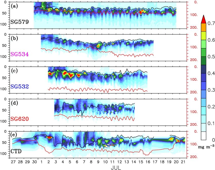
1450                                                        V. Thushara et al.: Chlorophyll distribution in the southern BoB

used to create a single glider dataset. The two-dimensional        lithogenic materials. The biogeochemical cycles are calcu-
(depth–time) optimally interpolated fields from each of the        lated with flexible nutrient stoichiometry. The phytoplankton
four gliders were combined into a single three-dimensional         class consists of three groups: small, large and diazotrophs.
(longitude–depth–time) gridded dataset by linearly interpo-        The small group represents the nanoplankton, which are
lating over longitude.                                             weakly limited by nutrients and strongly limited by graz-
   Observed fluorescence from gliders was corrected for            ing. The large group represents the microplankton, which are
non-photochemical quenching during daylight hours using            strongly limited by nutrients and weakly limited by grazing,
chlorophyll-to-backscatter ratios during night-time (Thoma-        with the ability to store iron internally. Diazotrophs (nitrogen
lla et al., 2018). The glider chlorophyll values exhibited         fixers) form a relatively small fraction of the total biomass
an offset similar to that found by Webber et al. (2014),           (Gnanadesikan et al., 2011). The model also includes dis-
with higher concentrations compared to the concurrent ob-          solved organic matter and heterotrophic biomass. The bio-
servations from the shipboard CTD. However, the glider             geochemical mechanisms consist of nitrogen fixation, deni-
data are reliable for explaining the processes underlying the      trification, gas exchange, atmospheric decomposition, scav-
bloom evolution, since the spatial and temporal variability        enging and sediment processes. Co-limitation by light and
of chlorophyll were consistent with the CTD observations.          nutrients controls the phytoplankton physiology and growth
For the present analysis, the glider data corrected for non-       (Geider et al., 1997) with a temperature dependency (Epp-
photochemical quenching were scaled to represent the in situ       ley, 1972). Grazing is parameterized using a size-based re-
chlorophyll value using the CTD data. An independent scale         lationship (Dunne et al., 2005) in which the large phyto-
factor was calculated for each glider’s ECOPuck using linear       plankton group dominates the ecosystem at high growth rates
regression with the available nearby CTD profiles, where the       and biomass, whereas the small phytoplankton group domi-
distance between the ship and glider is not more than a quar-      nates at low growth rates and biomass. Detritus production
ter of a degree, and the time difference is not more than an       is temperature dependent and calculated as a fraction of phy-
hour.                                                              toplankton (Dunne et al., 2005). Nitrification is inhibited by
                                                                   light (Ward et al., 1982). A detailed technical description of
2.2    Coupled physical–ecosystem model                            the ecosystem model is available in Dunne et al. (2010), and
                                                                   important model parameters are given in Table 1.
A coupled physical–ecosystem model was employed to                    The model configuration used in the present analysis is
study the observed chlorophyll distribution in the southern        similar to that in Thushara and Vinayachandran (2016). The
BoB during the BoBBLE field programme. The physical                physical model was spun up for a period of 10 years, start-
model is based on the Geophysical Fluid Dynamics Labo-             ing from a state of rest using climatological initial fields
ratory (GFDL) Modular Ocean Model Version 4 (MOM4p1;               for temperature and salinity (Conkright et al., 1998). This
Griffies et al., 2004), configured for the Indian Ocean region     was followed by a coupled spin-up for another 10 years, af-
extending from 30 to 120◦ E and 30◦ N to 30◦ S (Kurian and         ter switching on the ecosystem model. A stable annual cy-
Vinayachandran, 2007; Behara and Vinayachandran, 2016).            cle was obtained for both physical and biological fields af-
The horizontal resolution of the model is 0.25◦ , and the verti-   ter the spin-up, and this was followed by an interannual run
cal grid spacing is 5 m in the upper 60 m, increasing to 10 m      from 1 April 2015 to 31 December 2016. Nutrients for ini-
at 100 m depth, 20 m at 200 m depth and 700 m at 5000 m            tializing the ecosystem model were obtained from the World
depth, altogether forming 40 levels. The ETOPO5 dataset            Ocean Atlas (WOA09), and no-flux conditions were applied
with 5 min resolution is used to set up the model topography,      at the open boundaries. The model forcing fields include air
with the minimum depth of the ocean fixed at 30 m. A no-flux       temperature, specific humidity, surface pressure, downward
condition is applied across the model boundaries. Addition-        shortwave and longwave radiation fluxes, at hourly frequency
ally, a no-slip condition is applied to the closed western and     from Goddard Earth Observing System (GEOS) Modern-Era
northern boundaries. The open southern and eastern bound-          Retrospective analysis for Research and Applications, Ver-
aries consist of sponge layers where temperature and salin-        sion 2 (MERRA-2 ; Rienecker et al., 2011). Wind speed
ity fields are relaxed to climatology (Conkright et al., 1998),    and wind stress forcings were obtained from the Advanced
with a timescale of 30 days. The model mixing schemes are          SCATterometer (ASCAT; Figa-Saldaña et al., 2002). The
based on Large et al. (1994) and Chassignet and Garraffo           model freshwater forcings include daily precipitation from
(2001). Turbulent fluxes and upwelling longwave radiation          the Tropical Rainfall Measuring Mission (TRMM; Huff-
are calculated using the bulk formula (Large and Yeager,           man et al., 2007) and monthly climatological river runoff
2004), and the penetrative shortwave radiation is parameter-       from the Center for Sustainability and the Global Environ-
ized based on Morel and Antoine (1994).                            ment (SAGE; Vörösmarty et al., 1996). Weekly chlorophyll
   The ecosystem model used in this study is the Tracers           from the Sea-viewing Wide Field-of-View Sensor (SeaWiFS;
of Phytoplankton with Allometric Zooplankton (TOPAZ)               Sweeney et al., 2005) was used for the calculation of pene-
model (Dunne et al., 2010), consisting of 25 tracers, in-          trative shortwave radiation.
cluding micro- and macronutrients, carbon, oxygen, and

Biogeosciences, 16, 1447–1468, 2019                                                     www.biogeosciences.net/16/1447/2019/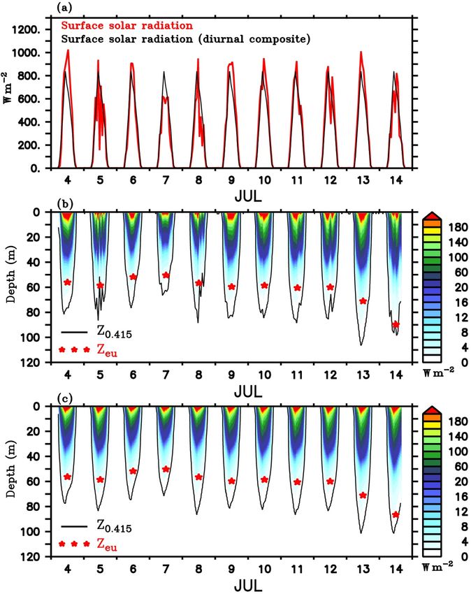
V. Thushara et al.: Chlorophyll distribution in the southern BoB                                                                1451

Table 1. Details of biological parameters used in the ecosystem model.

            Parameter    Description                                                                  Value
              Lg
            KNH          Half-saturation coefficient for ammonium uptake by large phytoplankton       6 × 10⁻⁷ mol NH4 kg−1
                 4
              Sm
            KNH          Half-saturation coefficient for ammonium uptake by small phytoplankton       2 × 10⁻⁷ mol NH4 kg−1
                 4
              Lg
            KNO          Half-saturation coefficient for nitrate uptake by large phytoplankton        6 × 10⁻⁶ mol NO3 kg−1
                 3
              Sm
            KNO          Half-saturation coefficient for nitrate uptake by small phytoplankton        2 × 10⁻⁶ mol NO3 kg−1
                 3
              Lg
            KPO          Half-saturation coefficient for phosphate uptake by large phytoplankton      6 × 10⁻⁷ mol PO4 kg−1
                 4
              Sm
            KPO          Half-saturation coefficient for phosphate uptake by small phytoplankton      2 × 10⁻⁷ mol PO4 kg−1
                 4
              Di
            KPO          Half-saturation coefficient for phosphate uptake by diazotrophs              6 × 10⁻⁷ mol PO4 kg−1
                 4
              Lg
            KSiO         Half-saturation coefficient for silicate uptake by large phytoplankton       1 × 10⁻⁶ mol SiO4 kg−1
                  4
              Lg
            KFe          Half-saturation coefficient for iron uptake by large phytoplankton           3 × 10⁻⁹ mol Fe kg−1
              Sm
            KFe          Half-saturation coefficient for iron uptake by small phytoplankton           1 × 10⁻⁹ mol Fe kg−1
              Di
            KFe          Half-saturation coefficient for iron uptake by diazotrophs                   3 × 10⁻⁹ mol Fe kg−1
              Lg
            PCmax        Maximum carbon assimilation rate for large phytoplankton                     1.5 × 10⁻⁵ s−1
              Sm
            PCmax        Maximum carbon assimilation rate for small phytoplankton                     1.5 × 10⁻⁵ s−1
              Di
            PCmax        Maximum carbon assimilation rate for diazotrophs                             0.6 × 10⁻⁵ s−1
             Lg
            θmax         Maximum chlorophyll-to-carbon ratio for large phytoplankton                  0.06 g Chl g C−1
             Sm
            θmax         Maximum chlorophyll-to-carbon ratio for small phytoplankton                  0.04 g Chl g C−1
             Di
            θmax         Maximum chlorophyll-to-carbon ratio for diazotrophs                          0.04 g Chl g C−1
            ζ            Cost of biosynthesis                                                         0.1
            κ            Eppley’s temperature coefficient                                             0.063 ◦ C−1
            λ0           Phytoplankton grazing rate constant at 0 ◦ C                                 0.19 day−1

3   Results and discussion                                               Colour Climate Change Initiative Version 3.1 (OC-CCI v3.1)
                                                                         merged product reveal that the southern bay exhibited high
The BoBBLE field programme coincided with a sup-                         chlorophyll levels during the BoBBLE period. The mean
pressed phase of the Boreal Summer Intraseasonal Oscilla-                chlorophyll concentration in the southern bay (82–92◦ E
tion (BSISO), when the convective activity was weak over                 and 4–12◦ N) averaged for the month of July was about
the southern BoB (see Fig. 4 of Vinayachandran et al., 2018).            0.2 mg m−3 , which is comparable to that of the previous
Precipitation was minimal during most of the observational               years.
period, until the establishment of the succeeding active phase
of the BSISO by the end of the programme. Surplus inso-                  3.1   Hydrography
lation associated with reduced atmospheric convection sug-
gests that light availability only played a minor role in lim-           To provide a dynamical context for the chlorophyll distribu-
iting the surface chlorophyll distribution. In the presence of           tion, the hydrography of the southern BoB during the BoB-
heavy cloud cover associated with the monsoon, light avail-              BLE period is briefly described here. Further details can be
ability is generally believed to limit the growth of phyto-              found in Vinayachandran et al. (2018) and Webber et al.
plankton in the Bay of Bengal. However, observational ev-                (2018). In response to the prevailing atmospheric conditions,
idence also shows that light is not an important limiting fac-           the upper ocean in the southern bay exhibited large spatial
tor in the low latitudes (Laws, 2013; Behrenfeld and Boss,               variability at seasonal and synoptic timescales. The climato-
2017), where the phytoplankton growth is mainly determined               logical distribution of surface temperature shows cooler wa-
by nutrient availability (Moore et al., 2013). According to              ters in the region of the SMC, creating an east–west con-
a recent study in the northern BoB by Jyothibabu et al.                  trast along 8◦ N (see Fig. 1 of Vinayachandran et al., 2018).
(2018), high PAR conditions were associated with low sur-                Weaker winds and higher insolation, associated with the sup-
face chlorophyll, and during low PAR conditions chlorophyll              pressed phase of BSISO during the observational period, re-
levels increased considerably.                                           sulted in high sea surface temperature (SST). The mean SST
   Monsoonal cloud cover, especially during the active                   obtained from the Group for High Resolution Sea Surface
phase of BSISO, limits the continuous sampling of ocean                  Temperature (GHRSST; Chao et al., 2009) dataset, averaged
colour from satellites, restricting the analysis of daily or             for the observational period (27 June–21 July 2016), was
weekly evolution of the chlorophyll blooms. Ocean colour                 ∼ 29.3 ◦ C at TSW and ∼ 0.5 ◦ C less at TSE, deviating from
data obtained from European Space Agency (ESA) Ocean                     the climatology. The mean sea surface salinity (SSS) from

www.biogeosciences.net/16/1447/2019/                                                              Biogeosciences, 16, 1447–1468, 2019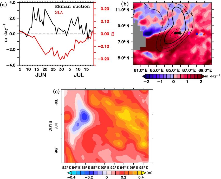
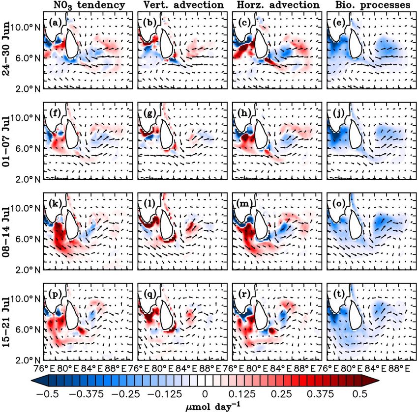
1452                                                            V. Thushara et al.: Chlorophyll distribution in the southern BoB

Figure 2. Depth–longitude sections of (a) temperature (◦ C) and
(b) salinity (psu) obtained from ocean gliders averaged for 3–
14 July, the common period when all the gliders performed data
sampling. Mean glider locations are marked at the top of each panel.
Red curves in (a) and (b) represent the thermocline and MLD re-
spectively. The thermocline is represented by the 20 ◦ C isotherm
(D20). MLD is calculated as the depth where density is equal to
the sea surface density plus an increase in density equivalent to a
reduction in temperature of 0.8 ◦ C.

the Soil Moisture Active Passive (SMAP; Fore et al., 2016)
mission was ∼33.3 psu at TSW, and farther east at TSE,
salinity was 0.8 psu higher.                                           Figure 3. Sea level anomalies (SLAs; m) and surface currents
   A depth–longitude section of temperature and salinity               (m s−1 ) from AVISO for the period 28 June to 9 July 2016. The
recorded by gliders, averaged for the period 3–14 July, is             glider locations are marked along 8◦ N (circles). Evolution of Sri
shown in Fig. 2. Gliders in the west (SG579 and SG532) ex-             Lanka Dome (SLD) is represented by the negative SLAs embedded
hibited higher SST and lower SSS compared to those in the              within the cyclonic circulation.
east (SG534 and SG620), consistent with the satellite obser-
vations. The thermocline, represented by the 20 ◦ C isotherm
(D20), exhibited an east–west dip along 8◦ N extending from            per ocean was relatively less dynamic, with weaker currents
TSW to 88◦ E, followed by a rise towards TSE (Fig. 2a). The            (0.1–0.3 m s−1 ) and positive sea level anomalies (10–20 cm).
western sector of the transect (TSW) lies within the SLD,                 The spatial variability in the upper-ocean dynamics of the
where open-ocean Ekman suction leads to the doming of the              BoB, determined by local and remote forcings associated
thermocline. At TSW, D20 was located at a depth of about               with the monsoon, influence the chlorophyll distribution as
80 m, as observed by SG579, and deepened towards the east.             well, which is of interest in the present study. The following
In the region of the high salinity core of the SMC intrusion           sections characterize the observed chlorophyll in the south-
(Fig. 2b), D20 was much deeper, located at a depth of about            ern bay in terms of intensities and the vertical distribution
180 m (SG532). At the eastern end of the transect (TSE), D20           during the BoBBLE period. The associated mechanisms de-
slightly shoaled by about 40 m, as observed by SG620.                  termining the chlorophyll distribution are analysed, combin-
   Circulation in the southern bay during the observational            ing hydrographical observations and results from an ecosys-
period is characterized by a strong cyclonic gyre in the re-           tem model.
gion of the SLD and the monsoon current which flows north-
eastward (Webber et al., 2018). During the beginning of the            3.2     Observed chlorophyll distribution
observational period, the SMC was strong, with surface ve-
locities ranging between 0.5 and 0.8 m s−1 (Fig. 3a–g). The            3.2.1    Surface bloom events
region of the SLD was characterized by strong negative sea
level anomalies (SLAs) of about −20 cm. By the end of the              The gliders cover an east–west transect across the regions
first week of July, the SMC weakened and shifted westward,             of the SLD and SMC (Fig. 1), providing time series mea-
reducing the zonal extent of the SLD (Fig. 3h–l). Farther east,        surements of chlorophyll. Surface layers remained weakly
towards the eastern edge of the monsoon current, the up-               productive during most of the observational period, however,

Biogeosciences, 16, 1447–1468, 2019                                                         www.biogeosciences.net/16/1447/2019/
V. Thushara et al.: Chlorophyll distribution in the southern BoB                                                                       1453

                                                                         Figure 5. Surface chlorophyll concentration (mg m−3 ) from ocean
                                                                         gliders (at 1 m) and the shipboard CTD (at 3 m). SG579 (black) falls
                                                                         within the region of SLD, SG534 (magenta) and SG532 (blue) along
                                                                         the path of SMC and SG620 (red) at the outer edge of SMC, as
                                                                         shown in Fig. 1. CTD (green) observations were collected along the
                                                                         8◦ N section, as described in Fig. 4.

                                                                         bloom during the same period (Fig. 4a; 30 June–2 July).
Figure 4. Time–depth sections of chlorophyll (mg m−3 ) from ocean        Chlorophyll concentration at the surface was ∼ 0.3 mg m−3
gliders (a–d) and CTD (e). The glider measurements are considered        on 30 June, increased to ∼ 0.7 mg m−3 on 1 July and re-
to be time series data for the locations shown in Fig. 1. CTD obser-     duced to ∼ 0.4 mg m−3 on 2 July (Fig. 5). CTD observations
vations were collected at TSW (85.3◦ E, 8◦ N) from 27 to 29 June,        were available within the dome on 28–29 June, before the
after which the ship sailed towards TSE (89◦ E, 8◦ N). From 3–           ship started moving eastwards from TSW. Until 29 June, sur-
15 July, time series measurements were made at TSE, after which
                                                                         face chlorophyll values were much lower (< 0.1 mg m−3 ),
the ship sailed back towards the west and reached TSW on 20 July.
The black curve represents the mixed layer depth, which is calcu-
                                                                         with higher concentrations mostly confined to a depth of
lated as the depth where density is equal to the sea surface density     about 30–60 m (Fig. 4e). Hence, it can be inferred that the
plus an increase in density equivalent to a reduction in temperature     surface chlorophyll bloom within the dome probably com-
of 0.8 ◦ C. The thermocline (red curve) is represented by the 20 ◦ C     menced on 30 June, peaked on 1 July and started decaying
isotherm (D20). Note that the y axis at the right side has a different   on 2 July. There were no glider observations of chlorophyll
scale.                                                                   before 30 June to corroborate the CTD data.
                                                                            The observed increase in surface chlorophyll at SG579 co-
                                                                         incided with the intensification of the SLD, characterized by
events of enhanced chlorophyll were observed at all of the               negative SLAs embedded within the cyclonic circulation to
four glider locations (Fig. 4a–d) as well as in the CTD data             the east of Sri Lanka (Fig. 3). Time series of minimum SLAs
(Fig. 4e). Surface chlorophyll concentrations from gliders               in the region of the dome show that the SLD attained its peak
and the CTD are shown in Fig. 5. During the beginning of                 by the end of June (Fig. 6a). Sea level anomalies decreased to
the observational period, concurrent occurrence of elevated              about −0.3 m on 30 June. The thermocline was shallow, lo-
chlorophyll levels was observed within the SLD and along                 cated at a depth of about 70 m, during the peak phase of the
the path of the SMC, as recorded by SG579, SG534 and                     surface chlorophyll bloom (1 July; Fig. 4). The doming of the
SG532. At SG620 (TSE), two events were recorded with rel-                thermocline indicates dynamical uplifting of the nutricline
atively weaker magnitudes of chlorophyll compared to the                 and enhanced nutrient concentrations in the euphotic zone
other glider locations. CTD measurements captured the sur-               (Wilson and Coles, 2005; Turk et al., 2001). The chlorophyll
face chlorophyll events in the region of the SMC on 1–2 July             bloom event was characterized by lower surface temperatures
and at TSE on 6–8 July, consistent with the glider obser-                (28.6 ◦ C) and higher surface salinities (33.95 psu) with up-
vations. The ship and glider were about 10 km apart during               sloping isotherms and isohalines (not shown), compared to
most of the observational period at TSE, and hence an exact              the period when the surface chlorophyll concentrations were
agreement in chlorophyll time series is not expected.                    weak. The decay of surface chlorophyll bloom after 2 July
   Within the SLD. Summer chlorophyll blooms in the re-                  (Fig. 5) followed the weakening of the dome (Fig. 6a). Sur-
gion of the SLD have been reported earlier using satellite               face temperature increased by 0.7 ◦ C, and surface salinity de-
images of ocean colour (Vinayachandran et al., 2004). The                creased by ∼ 1.5 psu on 3 July. The weakening of the dome
daily evolution of SLAs and currents from archiving, val-                indicates reduced upwelling of the subsurface nutrients. Nu-
idation, and interpretation of satellite oceanographic data              trient limitation restrains the growth of phytoplankton, lead-
(AVISO) show the intensification of the SLD during the                   ing to the decay of surface blooms, when the biological loss
early part (29 June–3 July) of the BoBBLE field programme                terms dominate. CTD observations within the dome until
(Fig. 3). Observations from SG579, which falls right inside              29 June, when the ship was at TSW, show that the subsur-
the dome, revealed the development of a surface chlorophyll              face chlorophyll concentrations were weak (< 0.5 mg m−3 )

www.biogeosciences.net/16/1447/2019/                                                              Biogeosciences, 16, 1447–1468, 2019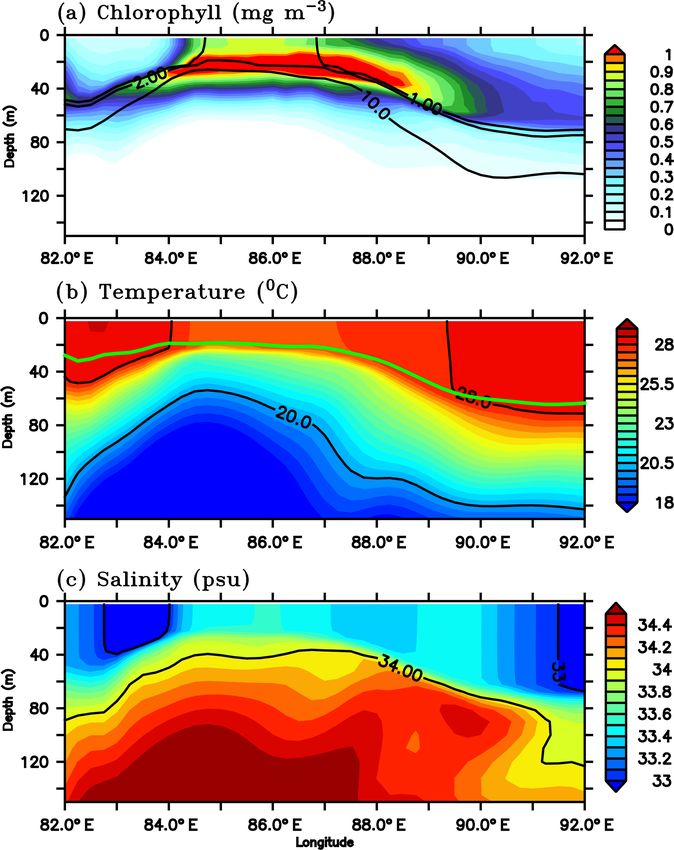
1454                                                         V. Thushara et al.: Chlorophyll distribution in the southern BoB

                                                                    is presumed to provide a favourable preconditioning by lift-
                                                                    ing the nitracline towards the surface.
                                                                       During the decaying phase of the SLD in July, Ekman
                                                                    vertical velocities were positive, with peak values of about
                                                                    2 m day−1 (Fig. 6a). This indicates the dominant influence of
                                                                    remote effects propagating from the eastern boundary of the
                                                                    BoB (Vinayachandran and Yamagata, 1998; Shankar et al.,
                                                                    2002; Wijesekera et al., 2016a; Burns et al., 2017; Webber
                                                                    et al., 2018). A time–longitude Hovmöller diagram of SLAs
                                                                    from AVISO during May–July along 8◦ N, between 80 and
                                                                    100◦ E, is shown in Fig. 6c. The decay period of the SLD
                                                                    coincides with the arrival of positive SLAs from east, rep-
                                                                    resenting the westward propagation of downwelling Rossby
                                                                    waves (Webber et al., 2018). Rossby waves propagating from
                                                                    the eastern boundary of the BoB can influence the depth of
                                                                    thermocline (nitracline) in the study region. This shows that,
                                                                    despite the Ekman suction, remote forcings contributed to
Figure 6. (a) Time series of Ekman vertical velocity (m day−1 ;     the weakening of the SLD and hence the chlorophyll distri-
black) around the location of SG579 (85–86◦ E, 7.5–8.5◦ N), and     bution. As far as surface chlorophyll is concerned, the prox-
the minimum SLAs (m; red) in the region of the Sri Lanka Dome       imity of nutricline to the surface is of primary concern. Re-
(SLD) from 5 June to 20 July. (b) Ekman vertical velocity aver-     sults from the ecosystem model have been used to identify
aged for the BoBBLE observational period (24 June–23 July) in the   the dominant forcings controlling the vertical displacement
southern BoB. Contours of SLAs are overlayed. (c) Time–longitude    of nitracline (see Sect. 3.3.1).
Hovmöller diagram of SLAs along 8◦ N between 81 and 100◦ E             Along the path of the SMC. Increased surface chlorophyll
from May to July.                                                   levels were observed at SG534 and SG532 on 1–2 July
                                                                    (Fig. 4b) and 2–4 July (Fig. 4c) respectively. Both gliders
                                                                    were located along the path of the SMC, with SG532 in
                                                                    the region of the subsurface high salinity core (Fig. 2b).
just before the surface chlorophyll event (Fig. 4e). This in-       Surface chlorophyll concentration peaked to about 0.35 and
dicates that the surface chlorophyll bloom is probably not a        0.4 mg m−3 at SG534 and SG532 respectively (Fig. 5). This
result of the vertical redistribution of subsurface phytoplank-     increase in chlorophyll was associated with lower tempera-
ton. On the other hand, the vertical transport of subsurface        tures (28.7 and 29.1 ◦ C for SG532 and SG534 respectively)
nutrients to the near-surface layers can favour the growth of       and higher salinities (34.4 and 34 psu for SG532 and SG534
phytoplankton in the given timescales (Laws, 2013), lead-           respectively) at the surface, compared to the period when the
ing to the intensification of surface chlorophyll. Though the       chlorophyll levels were weak.
evolution of observed chlorophyll follows the dynamics of              Along the path of the SMC, when the surface chlorophyll
the study region, the concurrent role of biological loss terms,     levels were high, the thermocline was deep (∼ 100–130 m
including grazing, mortality and sinking rates, cannot be ig-       at SG534 and ∼ 160–180 m at SG532), which is 40–100 m
nored, which requires additional data sampling.                     deeper than that in the region of the dome (Fig. 4a–c). The
   The southern BoB was characterized by cyclonic wind              spatial variability of thermocline is evident from the CTD ob-
stress curl, inducing Ekman suction during the field pro-           servations as well, showing a shallow thermocline during the
gramme. The vertical transport of nutrients to the surface          beginning (27–30 June) and end (20–21 July) of the field pro-
sunlit layers through Ekman suction favours the generation          gramme, when the ship was in the west, and a deeper thermo-
of phytoplankton blooms (Vinayachandran et al., 2004; Wi-           cline farther east (2–18 July; Fig. 4e). A deeper thermocline
jesekera et al., 2016a). Spatial distribution of Ekman vertical     generally indicates a deeper nitracline and stronger nutrient
velocities, calculated using ASCAT winds and averaged for           limitation in the surface layers. At the same time, the region
the BoBBLE observational period (24 June–23 July), indi-            of the SMC is also subject to an additional supply of biolog-
cates widespread upwelling in the southern BoB (Fig. 6b).           ically rich waters advected from the coasts of India and Sri
Time series of Ekman vertical velocities in the location            Lanka (Vinayachandran et al., 2004). In addition, the possi-
of SG579 show that Ekman suction peaked to about 2–                 bility of lateral advection of nutrients and chlorophyll gener-
3 m day−1 by mid-June (Fig. 6a). Ekman vertical velocities          ated within the SLD to the nearby glider locations cannot be
remained to be favourable for upwelling (0.4–0.7 m day−1 )          ignored (see Sect. 3.3.2).
during the period of surface bloom (30 June–2 July), though            Mixing events. Chlorophyll distribution observed outside
the magnitudes were relatively weaker. Strong upwelling in          the dome, farther east at TSE, differed from that in the re-
the second half of June, prior to the surface chlorophyll event,    gion of the SLD and SMC, in terms of intensity as well as the

Biogeosciences, 16, 1447–1468, 2019                                                     www.biogeosciences.net/16/1447/2019/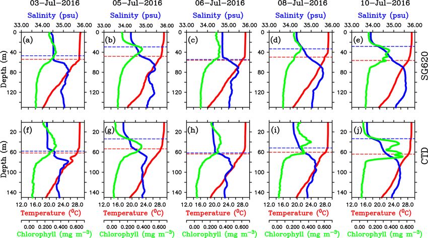
V. Thushara et al.: Chlorophyll distribution in the southern BoB                                                                 1455

                                                                        SG620 during different stages of the surface bloom evolu-
                                                                        tion are shown in Fig. 8a–e. During the peak of the sur-
                                                                        face chlorophyll blooms (3 and 6 July), the mixed layer was
                                                                        deep (∼ 50–55 m), with an almost uniform distribution of
                                                                        biophysical properties (Fig. 8a and c), and the isothermal
                                                                        layer was close to the mixed layer. The days following the
                                                                        peak in surface chlorophyll (4–5 and 8–10 July) were char-
                                                                        acterized by strong salinity stratification with the arrival of
                                                                        freshwater in the surface layers. Surface salinity decreased
Figure 7. Time series of wind speed (m s−1 ; red) from shipboard        by about 0.25 and 0.75 psu for the first and second events
AWS at TSE (89◦ E, 8◦ N). Surface salinity (psu; blue) and to-
                                                                        respectively (Fig. 8b and e). The mixed layer shoaled to
tal chlorophyll integrated over the mixed layer (mg m−2 ; green)
                                                                        ∼30 m, whereas the isothermal layer remained around the
is from SG620, deployed at TSE. MLD is calculated as the depth
where density is equal to the sea surface density plus an increase in   same depth (Fig. 8b, d and e). The associated development
density equivalent to a reduction in temperature of 0.8 ◦ C.            of barrier layers is noticeable, with a thickness of ∼ 25–
                                                                        30 m. Following the salinity stratification and barrier-layer
                                                                        formation, surface chlorophyll decreased by about 0.1 and
                                                                        0.15 mg m−3 during the first and second events respectively.
vertical structure. SG620 captured two events of enhanced               Vertical profiles obtained from the CTD at TSE for the same
surface chlorophyll: the first on 3 July and the second on              period are given in Fig. 8f–j. With the arrival of freshwa-
6–8 July (Fig. 4d). The surface chlorophyll concentrations              ter, surface salinity from the CTD decreased by about 0.25
were ∼0.3 mg m−3 during both the events (Fig. 5), charac-               and 0.5 psu during the first and second events respectively,
terized by low surface temperatures and high surface salin-             and the corresponding decrease in surface chlorophyll was
ities. The observed SST from SG620 was about 28.7 ◦ C on                0.1 and 0.15 mg m−3 respectively. The mixed layers shoaled
3 July and 28.8 ◦ C on 6 July. Surface salinities were about            by about 25–30 m, creating strong barrier layers (Fig. 8g, i
34.5 psu and 34.7 psu on 3 July and 6 July respectively. Tem-           and j). Even though high wind speed (∼ 10–12 m s−1 ) condi-
poral coverage of the first event is insufficient in explaining         tions prevailed during the decay period of the bloom, fresh-
its evolution, since the chlorophyll bloom decayed imme-                water induced stratification was strong enough to overcome
diately after 3 July, when the sampling began. Wind speed               the wind effect (Fig. 7). The observed biological response to
measured by the shipboard automatic weather station (AWS)               freshwater is similar to that in the northern bay, where strat-
was 5–9 m s−1 on 3 July (Fig. 7). A deeper mixed layer depth            ification inhibits the development of phytoplankton blooms
(MLD) of about 60 m during this period indicates that verti-            in the surface layers by restricting the vertical transport of
cal mixing is presumably the primary factor which favoured              subsurface nutrients and chlorophyll (Kumar et al., 2002).
the increase in surface chlorophyll. The second event was
captured by the CTD measurements as well (Fig. 4e), consis-             3.2.2   Deep chlorophyll maxima
tent with the glider data. This event coincided with a phase of
increasing wind speed of about 6–11 m s−1 (6–7 July; Fig. 7).           The formation of DCM is determined by a variety of mech-
Subsequent deepening of the mixed layer (∼ 70 m; Fig. 4d)               anisms, including an enhanced growth rate of phytoplank-
suggests the role of mixing and entrainment in triggering the           ton co-limited by light and nutrients at optimum depths,
intensification of surface chlorophyll. Enhanced vertical pro-          photoacclimation of pigment content, and physiologically
cesses favour intensification of surface chlorophyll by trans-          controlled swimming behaviours and buoyancy regulation
porting nutrients to the euphotic zone and by redistributing            (Cullen, 2015). The BoB is reported to have prominent DCM
the subsurface chlorophyll to the surface layers.                       (Murty et al., 2000; Madhu et al., 2006), which contribute
   The decay period of the observed surface chlorophyll                 to the column-integrated productivity (Gomes et al., 2000;
blooms (Fig. 5) coincided with the development of intermit-             Madhupratap et al., 2003; Li et al., 2012), with magnitudes
tent freshening events at the surface: the first on 4–5 July            often comparable to the highly productive Arabian Sea (Ku-
and the second on 7–10 July. The initial drop in surface                mar et al., 2009). However, little is known about the distribu-
salinity during the freshening events was ∼ 0.4 psu on 4 and            tion of subsurface chlorophyll in the BoB and the associated
7 July (Fig. 7). The surface chlorophyll decreased by about             processes, due to the lack of observations.
0.3 and 0.27 mg m−3 during the first and second freshening                 During the BoBBLE field programme, both the glider and
events respectively (Fig. 5). There was an overall reduction            CTD observations revealed the presence of prominent DCM
in total chlorophyll integrated over the mixed layer by about           in the southern bay (Figs. 4 and 9a). The chlorophyll max-
20 mg m−2 during both the freshening events (Fig. 7).                   ima were centred at a depth of about 20–50 m, mostly be-
   The freshening events were characterized by the forma-               low the mixed layer and above the thermocline (Anderson,
tion of barrier layers (Vinayachandran et al., 2018). Verti-            1969). Similar depth ranges of DCM were reported previ-
cal profiles of temperature, salinity and chlorophyll from              ously by Gomes et al. (2000) and Kumar et al. (2009) in the

www.biogeosciences.net/16/1447/2019/                                                           Biogeosciences, 16, 1447–1468, 2019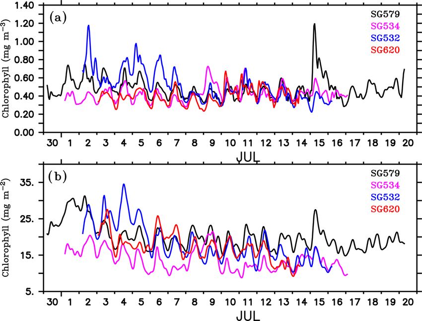
1456                                                              V. Thushara et al.: Chlorophyll distribution in the southern BoB

Figure 8. Daily mean vertical profiles of temperature (◦ C; red), salinity (psu; blue) and chlorophyll (mg m−3 ; green) for selected days from
(a–e) SG620 and (f–j) CTD. The blue dashed line indicates the mixed layer depth, which is calculated as the depth where density is equal to
the sea surface density plus an increase in density equivalent to a reduction in temperature of 0.8 ◦ C. The red dashed line indicates isothermal
layer depth (ILD) which is calculated as the depth where the temperature is cooler than SST by 0.8 ◦ C. The region between the MLD and
ILD represents the barrier layer.

                                                                              Vertical profiles of chlorophyll from the gliders during
                                                                           events of enhanced surface chlorophyll are shown in Fig. 10.
                                                                           The mean DCM were intense, located at a depth of about 20–
                                                                           30 m, in the region of the SLD and the SMC (Fig. 10a–c).
                                                                           The DCM became weaker, diffused and slightly deeper (30–
                                                                           40 m) at TSE (Fig. 10d and e). Intensification of DCM in the
                                                                           region of SLD can be related to the doming of thermocline.
                                                                           The vertical transport of nutrients is affected by the changes
                                                                           in thermocline depth, and hence, the variability of nutricline
                                                                           is found to be largely correlated with the variability of ther-
                                                                           mocline in the tropical oceans (Turk et al., 2001; Wilson and
                                                                           Adamec, 2002; Wilson and Coles, 2005). The shoaling of
                                                                           thermocline in the region of the SLD indicates an upward
                                                                           sloping of nutricline, indicating nutrient enrichment in the
                                                                           euphotic zone and enhanced accumulation of phytoplankton.
                                                                           At TSE (SG620), where the thermocline was deeper, mixing
Figure 9. (a) Concentration of deep chlorophyll maxima (mg m−3 )           often penetrated to deeper layers, pushing the mixed layer
and (b) depth-integrated (100 m) chlorophyll (mg m−2 ) from ocean          towards the DCM (Fig. 4d and e). This favours the dilution
gliders: SG579 (black), SG534 (magenta), SG532 (blue) and SG620            of DCM and a decrease in phytoplankton concentration at
(red).                                                                     the subsurface through mixing with the weakly productive
                                                                           surface layers, leaving a near-homogeneous distribution of
                                                                           chlorophyll within the water column (Fig. 10d and e).
                                                                              Subsurface chlorophyll concentrations were noticeably
BoB. Subsurface chlorophyll concentrations ranged from 0.3                 higher in the region of the SMC (Figs. 4c and 10c). Max-
to 1.2 mg m−3 (Fig. 9a), which were 2–3 times higher than                  imum intensities were recorded by SG532, with magni-
the surface values (Fig. 5). DCM were prominent in the re-                 tudes ranging from 0.7 to 1.2 mg m−3 on 2–7 July (Fig. 9a).
gion of the SLD and along the path of the SMC (Fig. 4a–                    Column-integrated chlorophyll was also observed to be the
c), whereas outside the dome, the subsurface concentrations                highest at SG532 (4 July), with total chlorophyll in the top
were weaker (Fig. 4d).                                                     100 m reaching as high as 35 mg m−2 (Fig. 9b), which is

Biogeosciences, 16, 1447–1468, 2019                                                               www.biogeosciences.net/16/1447/2019/
V. Thushara et al.: Chlorophyll distribution in the southern BoB 1457
Subsurface chlorophyll concentrations were observed to
intensify for shorter durations following the weakening of
surface blooms (Fig. 4). Increases in DCM concentrations
after the decay of surface blooms were about 0.13, 0.37
and 0.25 mg m−3 at SG534, SG532 and SG620 respectively
(Fig. 9a). In the region of the SLD (SG579), the subsurface
chlorophyll concentrations increased to ∼ 0.7 mg m−3 dur-
ing the peak phase of the surface bloom (1 July). During
the decaying phase of the surface bloom (2–5 July), these
high chlorophyll levels (0.7 mg m−3 ) were maintained at the
subsurface and weakened afterwards (Fig. 9a). This indicates
enhanced biological productivity at the subsurface, after the
triggering mechanisms inducing the surface blooms have
weakened. During the decaying phase of surface blooms, the
upper layers of the water column became less turbulent or
Figure 10. Vertical profiles of chlorophyll (mg m−3 ) from ocean more stably stratified (Fig. 8), inhibiting the vertical trans-
gliders during surface bloom events, as shown in Fig. 5. Individual port of nutrients and chlorophyll. For example, the surface
profiles are given in green, and the corresponding mean profiles are bloom event at SG620 weakened in response to the freshen-
given in red. Black dashed line represents the mixed layer depth, ing event on 8 July (Fig. 8b). Consequently, there was an in-
which is calculated as the depth where density is equal to the sea crease in DCM, which lasted for a period of about 2–3 days,
surface density plus an increase in density equivalent to a reduction from 10 to 12 July (Fig. 9a). The observed intensification of
in temperature of 0.8 ◦ C. DCM in the absence of surface chlorophyll can be explained
in terms of changes in subsurface irradiance levels. During
the decaying phase of the surface bloom, the self-shading ef-
comparable to the previously observed values in the BoB fect of surface phytoplankton weakens, enhancing the light
(Gomes et al., 2000; Madhupratap et al., 2003; Kumar et al., availability at the subsurface, which is examined in the fol-
2009; Li et al., 2012). The region of the SMC is charac- lowing section.
terized by the advection of upwelled chlorophyll-rich water
from the western coast of India and the southern coast of 3.2.3 Role of light limitation
Sri Lanka. An isolated maximum (1.2 mg m−3 ) in the DCM
was recorded by SG579 in the region of SLD in the lat- Chlorophyll interactive penetrative radiation was calculated
ter half of the observational period (15 July). However, in at TSE for the period 4–14 July, following the Morel and
the absence of surface blooms, the corresponding column- Antoine (1994) and Manizza et al. (2005) scheme as given
integrated chlorophyll was lower (28 mg m−2 ) compared to below:
the region of the SMC.
The core subsurface intrusion of the SMC, below the
I(z) = IIR · e−kIR z + IRED(z−1) · e−k(RED) 1z + IBLUE(z−1)
low salinity surface waters of the southern bay, was located
around SG532 during the observational period (Vinayachan- · e−k(BLUE) 1z , (1)
dran et al., 2018; Webber et al., 2018). The vertical salinity
structure reveals a high salinity core at 88◦ E, extending up where I(z) is the penetrative radiation at each depth level,
to a depth of about 180 m, with salinity values as high as IIR = I0 · (0.58) represents the infrared band, IVIS = I0 ·
35.8 psu (Fig. 2b). Arabian Sea water, which is rich in nutri- (0.42) represents the visible band and kIR = 2.86 m−1 is the
ents and chlorophyll sliding through the subsurface layers of light attenuation coefficient for the infrared band. The self-
the BoB, is presumed to contribute to the intensification of shading effect of phytoplankton is taken into account so that
the DCM at SG532, suggesting a key role of SMC intrusion at every vertical level (z), the available visible light is com-
in the biological budget of the southern bay. However, it may puted as a function of irradiance at the level just above (z−1).
be noted that the location of the subsurface high salinity core 1z is the thickness of each layer between two vertical levels,
was much deeper relative to the depth of DCM. Most of the which is 1 m in the present glider data. Visible light is split
high salinity intrusions at 88◦ E occurred below 80 m, in the into two averaged wavelength bands as given below,
deeper layers of the euphotic zone. Dynamics behind the dis-
tribution of the DCM in the region of the high salinity core IVIS
are intricate. Though the effect of lateral advection by the IRED = IBLUE = , (2)
2
SMC on DCM cannot be ignored, the possible contribution
of vertical processes in supplying the subsurface nutrients or where IRED and IBLUE are the irradiances in red and blue–
chlorophyll needs to be examined in detail. green bands respectively.
www.biogeosciences.net/16/1447/2019/ Biogeosciences, 16, 1447–1468, 20191458 V. Thushara et al.: Chlorophyll distribution in the southern BoB
The light attenuation coefficients for the two visible bands
is calculated as a function of chlorophyll concentration
([Chl]) as follows:
k(RED) = 0.225 + 0.037 · [Chl]0.629 , (3)
0.674
k(BLUE) = 0.0232 + 0.074 · [Chl] . (4)
Surface irradiance (I0 ) for the above calculations was ob-
tained from shipboard AWS (Fig. 11a) and chlorophyll from
SG620 (Fig. 4d). In order to exclude the effect of daily vari-
ation in surface irradiance, a diurnal composite of radiation
(Fig. 11a) for the period 4–14 July is also used for the cal-
culations. Photosynthetically active radiation (PAR) at each
vertical level (z) was estimated using the following expres-
sion:
2.5 × 10¹⁸
PAR(z) = Ivis(z) × , (5)
6.023 × 10²³
where Ivis( z) is the penetrative radiation (W m−2 ) in the
visible range calculated using the light model and 2.5 ×
1018 quanta s−1 W−1 is the conversion factor obtained from
Morel and Smith (1974). The depth of euphotic zone (Zeu )
was calculated as the depth at which light reduces to 1 %
of the surface PAR value. Considering the fact that phyto-
plankton sees the absolute light level and not the percent- Figure 11. (a) Surface solar radiation measured by the shipboard
age (Banse, 2004), the depth of threshold isolume (Z0.415 ) is AWS at TSE from 4 to 14 July (red), and the corresponding di-
urnal composite (black) calculated for the same period. Penetrative
taken as the depth where PAR is 0.415 E m−2 day−1 below
shortwave radiation is (W m−2 ) calculated following Morel and An-
which light is insufficient to support photosynthesis (Letelier
toine (1994) and Manizza et al. (2005) scheme using (b) observed
et al., 2004; Boss and Behrenfeld, 2010). An einstein (E) is a and (c) diurnal composite of radiation. Chlorophyll from SG620 is
mole of photons, i.e., 6.023 × 10²³ photons. used for the calculations. Photosynthetically active radiation (PAR;
Estimated penetrative radiation (W m−2 ) using the ob- E m−2 s−1 ) was estimated from the calculated penetrative radiation
served surface irradiance and the diurnal composite are in the visible range, following Morel and Smith (1974). The red
shown in Fig. 11b and c respectively. The corresponding stars in (b) and (c) represent daily averaged depth of euphotic zone
depths of euphotic zone and the threshold isolume obtained (Zeu , m) which is taken as the depth at which light reduces to 1 %
from the calculated PAR values are overlayed. Nearly 40 %– of the surface PAR value. The black contours in (b) and (c) repre-
60 % of the radiation was absorbed in the top 1 m of the water sent the depth of threshold isolume (Z0.415 , m) taken as the depth
column and 80 %–90 % in the top 30 m. Below the DCM, at which PAR is 0.415 E m−2 s−1 .
irradiance levels were substantially weaker (< 10 W m−2 ).
During the daylight hours of peak insolation, Z0.415 extended Following the decay of surface blooms owing to nutri-
to 70–110 m, with a well-defined diurnal cycle. During days ent limitation, Z0.415 and Zeu increased due to the penetra-
of enhanced surface chlorophyll, Z0.415 and Zeu were shal- tion of radiation to deeper layers (Perry et al., 2008). Z0.415
low. Z0.415 shoaled to a depth of about 70–80 m, and Zeu and Zeu deepened by about 25 and 10 m respectively on
was about ∼ 50 m during the chlorophyll bloom event at the 8 July (Fig. 11b). Enhanced light availability in the subsur-
surface on 6–7 July. The shoaling of the Z0.415 and Zeu in- face layers favours the intensification of DCM (Figs. 4d, e
dicates the self-shading effect of surface phytoplankton. El- and Fig. 8). It should be noted that the DCM may not repre-
evated levels of chlorophyll enhance the absorption of ra- sent a deep biomass maximum, as photoacclimation (Cullen,
diation in the surface layers (Fig. 11b). Calculations using 1982; Geider, 1987; Mateus et al., 2012) leads to changes
the diurnal composite of irradiance also give similar results in carbon-to-chlorophyll ratios. At the base of the euphotic
(Fig. 11c). Enhanced attenuation of radiation by near-surface layer, the cellular concentration of chlorophyll will increase
phytoplankton reduces the irradiance levels in the deeper as an adaptation to the lower irradiance levels (Cullen, 2015).
layers and strengthens the light limitation on phytoplankton
growth in the subsurface. As a result, bloom activity weakens
in the subsurface layers, despite the availability of nutrients.
Biogeosciences, 16, 1447–1468, 2019 www.biogeosciences.net/16/1447/2019/You can also read