The unidentified eruption of 1809: a climatic cold case - CP
←
→
Page content transcription
If your browser does not render page correctly, please read the page content below
Clim. Past, 17, 1455–1482, 2021
https://doi.org/10.5194/cp-17-1455-2021
© Author(s) 2021. This work is distributed under
the Creative Commons Attribution 4.0 License.

The unidentified eruption of 1809: a climatic cold case
Claudia Timmreck1 , Matthew Toohey2 , Davide Zanchettin3 , Stefan Brönnimann4 , Elin Lundstad4 , and Rob Wilson5
1 The  Atmosphere in the Earth System, Max Planck Institute for Meteorology, Bundesstr. 53, 20146 Hamburg, Germany
2 Department   of Physics and Engineering Physics, University of Saskatchewan, Saskatoon, Canada
3 Department of Environmental Sciences, Informatics and Statistics, University Ca’ Foscari of Venice, Mestre, Italy
4 Institute of Geography Climatology and Oeschger Centre for Climate Change Research,

University of Bern, 3012 Bern, Switzerland
5 School of Earth & Environmental Sciences, University of St. Andrews, St. Andrews, United Kingdom

Correspondence: Claudia Timmreck (claudia.timmreck@mpimet.mpg.de)

Received: 20 January 2021 – Discussion started: 26 January 2021
Revised: 25 May 2021 – Accepted: 7 June 2021 – Published: 13 July 2021

Abstract. The “1809 eruption” is one of the most recent           tions between the N-TREND NH temperature reconstruction
unidentified volcanic eruptions with a global climate impact.     and the model simulations are weak in terms of the ensemble-
Even though the eruption ranks as the third largest since 1500    mean model results, individual model simulations show good
with a sulfur emission strength estimated to be 2 times that      correlation over North America and Europe, suggesting the
of the 1991 eruption of Pinatubo, not much is known of            spatial heterogeneity of the 1810 cooling could be due to in-
it from historic sources. Based on a compilation of instru-       ternal climate variability.
mental and reconstructed temperature time series, we show
here that tropical temperatures show a significant drop in re-
sponse to the ∼ 1809 eruption that is similar to that produced
by the Mt. Tambora eruption in 1815, while the response           1   Introduction
of Northern Hemisphere (NH) boreal summer temperature
is spatially heterogeneous. We test the sensitivity of the cli-   The early 19th century (∼ 1800–1830 CE), at the tail end of
mate response simulated by the MPI Earth system model to          the Little Ice Age, marks one of the coldest periods of the
a range of volcanic forcing estimates constructed using es-       last millennium (e.g., Wilson et al., 2016; PAGES 2k Con-
timated volcanic stratospheric sulfur injections (VSSIs) and      sortium, 2019) and is therefore of special interest in the study
uncertainties from ice-core records. Three of the forcing re-     of inter-decadal climate variability (Jungclaus et al., 2017). It
constructions represent a tropical eruption with an approx-       was influenced by strong natural forcing: a grand solar min-
imately symmetric hemispheric aerosol spread but different        imum (Dalton Minimum, ∼ 1790–1820 CE) and simultane-
forcing magnitudes, while a fourth reflects a hemispherically     ously a cluster of very strong tropical volcanic eruptions that
asymmetric scenario without volcanic forcing in the NH ex-        includes the widely known Mt. Tambora eruption in 1815,
tratropics. Observed and reconstructed post-volcanic surface      an unidentified eruption estimated to have occurred in 1808
NH summer temperature anomalies lie within the range of           or 1809, and a series of eruptions in the 1820s and 1830s.
all the scenario simulations. Therefore, assuming the model       Brönnimann et al. (2019a) point out that this sequence of vol-
climate sensitivity is correct, the VSSI estimate is accurate     canic eruptions influenced the last phase of the Little Ice Age
within the uncertainty bounds. Comparison of observed and         by not only leading to global cooling but also by modifying
simulated tropical temperature anomalies suggests that the        the large-scale atmospheric circulation through a southward
most likely VSSI for the 1809 eruption would be somewhere         shift of low-pressure systems over the North Atlantic related
between 12 and 19 Tg of sulfur. Model results show that NH        to a weakening of the African monsoon and the Atlantic–
large-scale climate modes are sensitive to both volcanic forc-    European Hadley cell (Wegmann et al., 2014).
ing strength and its spatial structure. While spatial correla-       The Mt. Tambora eruption in April 1815 was the largest
                                                                  in the last 500 years and had substantial global climatic

Published by Copernicus Publications on behalf of the European Geosciences Union.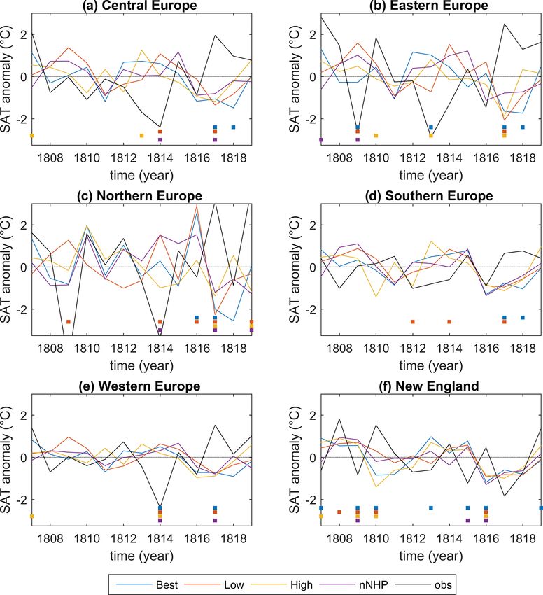
1456                                              C. Timmreck et al.: The unidentified eruption of 1809: a climatic cold case

and societal effects (e.g., Oppenheimer, 2003; Brönnimann         has been given to characterizing and understanding the short-
and Krämer, 2016; Raible et al., 2016). In contrast to the        term climatic anomalies that specifically followed the 1809
Mt. Tambora eruption, little is known about the 1809 erup-        eruption. Available observations and reconstructions indicate
tion. Although there is no historical source reporting a strong   ambiguous signals in NH land-mean summer temperatures
volcanic eruption in 1809, its occurrence is indubitably          reconstructed from tree-ring data for this period. For exam-
brought to light by ice-core sulfur records, which clearly        ple, Schneider et al. (2017) found that, among the 10 largest
identify a peak in volcanic sulfur in 1809/1810 (Dai et al.,      eruptions of the past 2500 years, the 1809 event was one of
1991). Simultaneous signals in both Greenland and Antarctic       two that did not produce a significant “break” in the tem-
ice cores with similar magnitude are consistent with a trop-      perature time series. While the temperature reconstruction
ical origin, and analysis of sulfur isotopes in ice cores sup-    reports cooling in 1809/1810, Schneider et al. (2017) note
ports the hypothesis of a major volcanic eruption with strato-    that reconstructed temperatures did not return to their clima-
spheric injection (Cole-Dai et al., 2009).                        tological mean after the initial drop and remained low un-
   Based on ice-core sulfur records from Antarctica and           til the Mt. Tambora eruption in 1815. Hakim et al. (2016)
Greenland, the 1809 eruption is estimated to have injected        presented multivariate reconstructed fields for the 1809 vol-
19.3 ± 3.54 Tg of sulfur (S) into the stratosphere (Toohey        canic eruption from the last millennium climate reanalysis
and Sigl, 2017). This value is roughly 30 % less than the         (LMR) project. They found abrupt global surface cooling
estimate for the 1815 Mt. Tambora eruption and roughly            in 1809, which was reinforced in 1815. The post-volcanic
twice that of the 1991 Pinatubo eruption. Accordingly, the        global-mean 2 m temperature anomalies, however, show a
1809 eruption produced the second-largest volcanic strato-        wide spread of up to 0.3 ◦ C in the LMR between ensem-
spheric sulfur injection (VSSI) of the 19th century and the       ble members and experiments using different combinations
sixth largest of the past 1000 years. For comparison, the Ice-    of calibration data for the proxy system models and prior
core Volcanic Index 2 (IVI2) database (Gao et al., 2008)          data in the reconstruction. Using the LMR paleoenvironmen-
estimates that the 1809 eruption injected 53.7 Tg of sulfate      tal data assimilation framework, Zhu et al. (2020) demon-
aerosols, which corresponds to 13.4 Tg S. While smaller than      strate that some of the known discrepancies between tree-
the estimate of Toohey and Sigl (2017), the IVI2 value lies       ring data and paleoclimate models can partly be resolved by
within the reported 2σ uncertainty range. Uncertainties in        assimilating tree-ring density records only and focusing on
VSSI and related uncertainties in the radiative impacts of        growing-season temperatures instead of annual temperature
the volcanic aerosol could be relevant for the interpretation     while performing the comparison at the proxy locales. How-
of post-volcanic climate anomalies, as recently discussed for     ever, differences remain for large events like the Mt. Tambora
the 1815 Mt. Tambora eruption and the “year without sum-          1815 eruption.
mer” in 1816 (Zanchettin et al., 2019; Schurer et al., 2019).        In this study, we investigate the climate impact of the 1809
   While the location and the magnitude of the 1809 eruption      eruption by using Earth system model ensemble simulations
are unknown, its exact timing is also uncertain. A detailed       and by analyzing new and existing observational and proxy-
analysis of high-resolution ice-core records points to an erup-   based datasets. We explore how uncertainties in the magni-
tion in February 1809 ± 4 months (Cole-Dai, 2010), which is       tude and spatial structure of the forcing propagate to the mag-
consistent with the timing implied by other high-resolution       nitude and ensemble variability of post-eruption regional and
ice-core records (Sigl et al., 2013, 2015; Plummer et al.,        hemispheric climate anomalies.
2012). Observations from South America of atmospheric                In Sect. 2, we briefly describe the applied methods, model,
phenomena consistent with enhanced stratospheric aerosol          experiments, and datasets. Section 3 provides an overview of
(Guevara-Murua et al., 2014) suggest a possible eruption          the reconstructed and observed climate effects of the 1809
in late November or early December 1808 (4 December               eruption, while Sect. 4 presents the main results of the model
1808 ± 7 d), although there is no direct link between these       experiments including a model–data intercomparison. The
observations and the ice-core sulfate signals. Chenoweth          results are discussed in Sect. 5. The paper ends with a sum-
(2001) proposed an eruption date of March–June 1808 based         mary and conclusions (Sect. 6).
on a sudden cooling in Malaysian temperature data and max-
imum cooling of marine air temperature in 1809. Such un-
certainty in the eruption date has implications for the asso-     2     Methods and data
ciated spatiotemporal pattern of aerosol dispersal as well as
hemispheric and global climate impacts (Toohey et al., 2011;      2.1     Methods
Timmreck, 2012). The climatic impacts of the 1809 erup-           2.1.1    Model
tion have been mostly studied in the context of the early 19th
century volcanic cluster (e.g., Cole-Dai et al., 2009; Zanchet-   We use the latest low-resolution version of the Max Planck
tin et al., 2013, 2019; Anet et al., 2014; Winter et al., 2015;   Institute Earth System Model (MPI-ESM1.2-LR; Mauritsen
Brönnimann et al., 2019a) or multi-eruption investigations        et al., 2019), an updated version of the MPI-ESM used in the
(e.g., Fischer et al., 2007; Rao et al., 2017). Less attention    Coupled Model Intercomparison Project Phase 5 (CMIP5)

Clim. Past, 17, 1455–1482, 2021                                                     https://doi.org/10.5194/cp-17-1455-2021
C. Timmreck et al.: The unidentified eruption of 1809: a climatic cold case                                                1457

(Giorgetta et al., 2013). The applied MPI-ESM1.2 configu-         albedo, and scattering asymmetry factors are derived for
ration is one of the two reference versions used in the Cou-      pre-defined wavelength bands and latitudes. Volcanic strato-
pled Model Intercomparison Project Phase 6 (CMIP6; see            spheric sulfur injection (VSSI) values for the simulations
Eyring et al., 2016). It consists of four components: the atmo-   performed in this work are taken from the eVolv2k recon-
spheric general circulation model ECHAM6 (Stevens et al.,         struction based on sulfate records from various ice cores from
2013), the ocean–sea ice model MPIOM (Jungclaus et al.,           Greenland and Antarctica (Toohey and Sigl, 2017). Com-
2013), the land component JSBACH (Reick et al., 2013), and        pared to prior volcanic reconstructions, eVolv2k includes im-
the marine biogeochemistry model HAMOCC (Ilyina et al.,           provements of the ice-core records in terms of synchroniza-
2013). JSBACH is directly coupled to the ECHAM6.3 model           tion and dating, as well as in the methods used to estimate
and includes dynamic vegetation, whereas HAMOCC is di-            VSSI from them.
rectly coupled to the MPIOM. ECHAM6 and MPIOM are in                 Consistent with the estimated range given by Cole-Dai
turn coupled through the OASIS3-MCT coupler software. In          (2010) and the convention for unidentified eruptions used
MPI-ESM1.2, ECHAM6.3 is used, which is run with a hor-            by Crowley and Unterman (2013), the eruption date of the
izontal resolution in the spectral space of T63 (∼ 200 km)        unidentified 1809 eruption is set to occur on 1 January 1809
and with 47 vertical levels up to 0.01 hPa and 13 model           located at the Equator. The eVolv2k best estimate for the
levels above 100 hPa. In ECHAM6.3 aerosol microphysical           VSSI of the 1809 eruption is 19.3 Tg S, with a 1σ uncertainty
processes are not included. The radiative forcing of the vol-     of ±3.54 Tg S based on the variability between individual
canic aerosol is prescribed by monthly and zonal-mean opti-       ice-core records and model-based estimates of error due to
cal parameters, which are generated with the Easy Volcanic        the limited hemispheric sampling provided by ice sheets. To
Aerosol forcing generator (EVA; Toohey et al., 2016); see         incorporate this uncertainty into climate model simulations,
Sect. 2.1.2. The MPIOM, which is run in its GR15 configu-         we constructed aerosol forcing time series using the cen-
ration with a nominal resolution of 1.5◦ around the Equator       tral (or best) VSSI estimate, as well as versions which per-
and 40 vertical levels, has remained largely unchanged with       turbed the central estimate by adding and subtracting 2 times
respect to the CMIP5 version. Several revisions with respect      the estimated uncertainty (±2σ ) from the central VSSI esti-
to the MPI-ESM CMIP5 version have, however, been made             mate. These three forcing sets are hereafter termed “Best”,
for the atmospheric model including a new representation of       “High”, and “Low”, respectively. Constructed in this man-
radiation transfer, land physics, and biogeochemistry compo-      ner, the range from Low to High forcing should roughly span
nents as well as the ocean carbon cycle. A detailed descrip-      a 95 % confidence interval of the global-mean aerosol forc-
tion of all updates is given in Mauritsen et al. (2019). Previ-   ing.
ous studies have successfully shown that MPI-ESM is espe-            There are other important sources of uncertainty in the re-
cially well-suited for paleo-applications and has been widely     construction of stratospheric aerosol other than that related
tested and employed in the context of the climate of the last     to the magnitude of the sulfur deposition. For example, the
millennium (e.g., Jungclaus et al., 2014; Zanchettin et al.,      transport of aerosol from the tropics to each hemisphere
2015; Moreno-Chamarro et al., 2017).                              has been seen to be quite variable for the tropical eruptions
                                                                  of Pinatubo in June 1991, El Chichón in April 1982, and
2.1.2   Forcing
                                                                  Agung in March 1963, which likely arises due to the par-
                                                                  ticular meteorological conditions at the time of the eruption
The applied volcanic forcing is compiled with the Easy Vol-       (Robock, 2000). While the 1991 Pinatubo eruption produced
canic Aerosol (EVA) forcing generator (Toohey et al., 2016).      an aerosol cloud that spread relatively evenly to each hemi-
EVA provides an analytic representation of volcanic strato-       sphere, the aerosol from the 1982 El Chichón eruption and
spheric aerosol forcing, prescribing the aerosol’s radiative      the 1963 Agung eruption was heavily biased to one hemi-
properties and primary modes of their spatial and tempo-          sphere (Fig. S2 in the Supplement). Furthermore, the life-
ral variability. Although EVA represents an idealized forc-       time, evolution, and spatial structure of aerosol properties
ing approach, its forcing estimates lie within the multi-model    may vary significantly as a result of the injection height of
range of global aerosol simulations for the Tambora erup-         the volcanic plume (Toohey et al., 2019; Marshall et al.,
tion (Zanchettin et al., 2016; Clyne et al., 2021). This also     2019). Recently, Yang et al. (2019) pointed out that an ac-
permits the compilation of physically consistent forcing esti-    curate reconstruction of the spatial forcing structure of vol-
mates for historic eruptions. EVA uses sulfur dioxide (SO2 )      canic aerosol is important to get a reliable climate response.
injection time series as input and applies a parameterized        Motivated in large part by the post-1809 surface tempera-
three-box model of stratospheric transport to reconstruct the     ture anomalies to be discussed below, which include strong
space–time structure of sulfate aerosol evolution. Simple         cooling in the tropics and a muted NH mean temperature sig-
scaling relationships serve to construct stratospheric aerosol    nal, we constructed a fourth forcing set, which is identical to
optical depth (SAOD) at 0.55 µm and aerosol effective ra-         the Best forcing in the tropics and in the Southern Hemi-
dius from the stratospheric sulfate aerosol mass, from which      sphere (SH) but has the aerosol mass in the NH extratropics
wavelength-dependent aerosol extinction, single-scattering        completely removed, creating a strongly asymmetric forc-

https://doi.org/10.5194/cp-17-1455-2021                                                      Clim. Past, 17, 1455–1482, 2021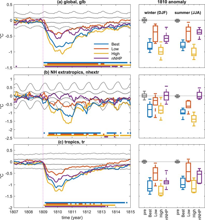
1458                                              C. Timmreck et al.: The unidentified eruption of 1809: a climatic cold case

ing structure. This forcing scenario, which we call “no-NH        we have produced 10 realizations branched off every 100 to
plume” or “nNHP” in the following, should be interpreted          200 years from an unperturbed 1200-year-long pre-industrial
as a rather extreme “end-member” in terms of NH forcing.          control run (constant forcing, excluding background volcanic
The lack of aerosol for the NH in this constructed forcing is     aerosols) to account for internal climate variability. All simu-
clearly inconsistent with the polar ice-core records of sulfate   lations were initialized on 1 January 1800 with constant pre-
deposition from the 1809 eruption, which suggests roughly         industrial forcing except for stratospheric aerosol forcing.
equal deposition between Greenland and Antarctica over a
similar duration as other typical tropical eruptions, indicat-    2.2     Data
ing a long-lasting and global aerosol spread. Due to uncer-
tainties in the conversion of ice-core sulfate to hemispheric     2.2.1    Temperature reconstructions
aerosol burden and radiative forcing (Toohey and Sigl, 2017;
                                                                  Tropical temperature reconstructions
Marshall et al., 2020), it is not impossible that the radiative
forcing from the 1809 eruption aerosol was characterized          In our study, we compare three different sea surface temper-
by some degree of hemispheric asymmetry in reality. Still,        ature (SST) reconstructions with the MPI-ESM simulations.
the nNHP forcing presented here should be interpreted as a        The temperature reconstruction TROP is a multi-proxy trop-
rather unlikely scenario for the 1809 eruption. Here we ex-       ical (30◦ N–30◦ S, 34◦ E–70◦ W) annual SST reconstruction
plore the impact of this forcing scenario as an extreme ideal-    between 1546 and 1998 (D’Arrigo et al., 2009). TROP con-
ized form of hemispheric asymmetry that might conceivably         sists of 19 coral, tree-ring, and ice-core proxies located be-
play some role in the response to the 1809 eruption and is di-    tween 30◦ N and 30◦ S. The records were selected on the
rectly applicable to “unipolar” tropical eruptions like Agung     basis of data availability, dating certainty, annual or higher
(1963) and El Chichón (1982).                                     resolution, and a documented relationship with temperature.
   Time series of global-mean and zonal-mean SAOD at              It shows annual- to multi-decadal-scale variability and ex-
0.55 µm for the different 1809 aerosol forcing scenarios dis-     plains 55 % of the annual variance in the most replicated
cussed above are shown in Fig. 1, together with the Best          period of 1897–1981. Further, 400-year-long spatially re-
scenario after the Mt. Tambora eruption. Peak global-mean         solved tropical SST reconstructions for four specific regions
SAOD values following the 1809 eruption range from 0.17           in the Indian Ocean (20◦ N–15◦ S, 40–100◦ E), the west-
to 0.33 from the Low to High scenarios, roughly correspond-       ern (25◦ N–25◦ S, 110–155◦ E) and eastern Pacific (10◦ N–
ing to forcing from a little stronger than that from the 1991     10◦ S, 175◦ E–85◦ W), and the western Atlantic (15–30◦ N,
Pinatubo eruption to a little weaker than the 1815 Mt. Tamb-      60–90◦ W) were compiled by Tierney et al. (2015) based
ora eruption, respectively. The nNHP scenario produces a          on 57 published and publicly archived marine paleoclimate
global-mean SAOD that peaks at a value of 0.21, i.e., be-         datasets. The four regions were selected based on the avail-
tween the Low and Best scenarios, and decays in a manner          ability of nearby coral sampling sites and an analysis of spa-
very similar in magnitude to the Low scenario. The latitu-        tial temperature covariance. An even more regionally specific
dinal spread of aerosol is relatively evenly split between the    SST reconstruction was developed by D’Arrigo et al. (2006)
NH and SH in the Best, Low, and High scenarios, with off-         for the Indo-Pacific warm pool region (15◦ S–5◦ N, 110–
sets in the timing of the peak hemispheric SAOD resulting         160◦ E) using annually resolved teak-ring-width and coral
from the parameterized seasonal dependence of stratospheric       δ 18 O records. This September–November mean SST recon-
transport in EVA. After the removal of aerosol mass from the      struction dates from 1782–1992 CE and explains 52 % of the
NH extratropics in the construction of the nNHP scenario,         SST variance in the most replicated period. This record was
the SAOD is predictably negligible in the NH extratropics,        used in the D’Arrigo et al. (2009) TROP reconstruction.
and a strong gradient in SAOD is produced at 30◦ N.
                                                                  Northern Hemisphere extratropical temperature
2.1.3   Experiments                                               reconstruction

We have performed ensemble simulations of the early 19th          We compare our climate simulations of the early 19th cen-
century with the MPI-ESM1.2-LR for each of the four forc-         tury with four near-surface air temperature (SAT) reconstruc-
ing scenarios for the 1809 eruption (Best, High, Low, and         tions, which have all been used to assess the impacts of
nNHP). All simulations also include the eVolv2k Best forc-        volcanic eruptions on surface temperature. The N-TREND
ing estimate for the Mt. Tambora eruption from 1815 on-           (Northern Hemisphere Tree-Ring Network Development) re-
wards. Related experiments using a range of different forc-       constructions (Wilson et al., 2016; Anchukaitis et al., 2017)
ing estimates for the 1815 Mt. Tambora eruption were used         are based on 54 published tree-ring records and use different
in Zanchettin et al. (2019) and Schurer et al. (2019) to in-      parameters as proxies for temperature. A total of 11 of the
vestigate the role of volcanic forcing uncertainty in the cli-    records are derived from ring width (RW), 18 are from max-
mate response to the 1815 Mt. Tambora eruption, in particu-       imum latewood density (MXD), and 25 are mixed records
lar the “year without summer” in 1816. For each experiment        which consist of a combination of RW, MXD, and blue in-

Clim. Past, 17, 1455–1482, 2021                                                      https://doi.org/10.5194/cp-17-1455-2021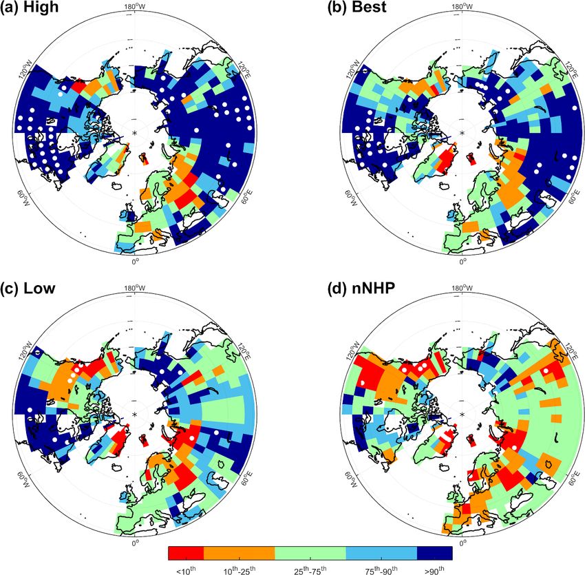
C. Timmreck et al.: The unidentified eruption of 1809: a climatic cold case                                                              1459

Figure 1. Volcanic radiative forcing. Global stratospheric aerosol optical depth (SAOD) at 0.55 µm based on eVolv2k VSSI estimates (Toohey
and Sigl, 2017) and calculation with the volcanic forcing generator EVA (Toohey et al., 2016) for the four different forcing scenarios (“Best”,
“Low”, “High”, and “nNHP”) for the 1809 eruption and the Best forcing scenario for the Mt. Tambora eruption. Bottom: spatial and temporal
distribution of a zonal-mean stratospheric SAOD for the four experiments.

tensity (BI) data (see Wilson et al., 2016, for details). The             three isotope series from Greenland ice cores (DYE3, GRIP,
N-TREND database domain covers the NH midlatitudes be-                    Crete). NVOLC was generated using a nested approach and
tween 40 and 75◦ N, with at least 23 records extending back               includes only chronologies which encompass the full time
to at least 978 CE. Two versions of the N-TREND recon-                    period between today and the 13th century. The tempera-
structions are used herein. N-TREND (N), detailed in Wilson               ture reconstruction by Schneider et al. (2015) is based on
et al. (2016), is a large-scale mean composite May–August                 15 MXD chronologies distributed across the NH extratrop-
temperature reconstruction derived from averaging the 54                  ics. All the temperature reconstructions show distinct short-
tree-ring records weighted to four longitudinal quadrats, with            time cooling after the largest eruptions of the Common Era.
separate nested calibration and validation performed as each              However, Schneider et al. (2017) point to a notable spread
shorter record is removed back in time. N-TREND (S), de-                  in the post-volcanic temperature response across the differ-
tailed in Anchukaitis et al. (2017), is a spatial reconstruction          ent reconstructions. This has various possible explanations,
of the same season derived by using point-by-point multiple               including the different parameters used, the spatial domain
regression (Cook et al., 1994) of the tree-ring proxy records             of the reconstruction, the method(s) used for detrending, and
available within 1000 to 2000 km of the center point of each              choices made in the network compilations.
5 × 5◦ instrumental grid cell. For each gridded reconstruction
a similar nesting procedure was used as Wilson et al. (2016).
Herein, we use the average of all the grid point reconstruc-              2.2.2    Observed temperatures
tions for the periods during which the validation reduction of            Surface air temperature from English East India
error (RE – Wilson et al., 2016) was greater than zero. The               Company ship logs
NVOLC reconstruction (Guillet et al., 2017) is an NH sum-
mer temperature reconstruction over land (40–90◦ N) com-                  Brohan et al. (2012) compiled an early observational dataset
posed of 25 tree-ring chronologies (12 MXD, 13 TRW) and                   of weather and climate between 1789 and 1834 from records
                                                                          of the English East India Company (EEIC), which are

https://doi.org/10.5194/cp-17-1455-2021                                                                Clim. Past, 17, 1455–1482, 2021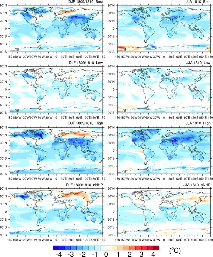
1460                                               C. Timmreck et al.: The unidentified eruption of 1809: a climatic cold case

archived in the British Library. The records include 891           rogate ensembles is sampled from the control run, each iden-
ships’ logbooks of voyages from England to India or China          tified by a randomly chosen year as a reference for the erup-
and back containing daily instrumental measurements of             tion. Ensemble means and spreads (defined by 5th and 95th
temperature and pressure, as well as wind-speed estimates.         percentiles) of such surrogate ensembles provide an empiri-
Several thousand weather observations could be gained from         cal probability distribution that is used to determine the range
these ship voyages across the Atlantic and Indian oceans,          of intrinsic variability, which is illustrated by the associ-
providing a detailed view of the weather and climate in the        ated 5th–95th percentile ranges. Differences between the vol-
early 19th century. Brohan et al. (2012) found that mean tem-      canically forced ensembles and the surrogate ensembles are
peratures expressed a modest decrease in 1809 and 1816 as          tested statistically through the Mann–Whitney U test (fol-
a likely consequence of the two large tropical volcanic erup-      lowing, e.g., Zanchettin et al., 2019). When the ensembles
tions during the period. Following Brohan et al. (2012), here      are compared with a one-value target, either an anomaly from
we calculate temperature anomalies from the SAT measure-           reconstructions and observations or a given reference (e.g.,
ments recorded in the EEIC logs. We account for the rel-           zero), the significance of the difference between the ensem-
atively sparse and irregular spatial and temporal sampling         ble and the target is determined based on whether the lat-
by computing for each measurement its anomaly from the             ter exceeds a given percentile range from the ensemble (e.g.,
HadNMAT2 night marine air temperature climatology (Kent            the interquartile or the 5th–95th percentile range) or, alterna-
et al., 2013). The SAT anomalies were then binned according        tively, based on a t test.
to the month, year, and location and averaged. We present the          Integrated spatial analysis between the simulations and the
data as mean temperature anomalies for the tropics (20◦ S to       N-TREND (S) gridded reconstruction is performed through a
20◦ N) in monthly or annual means. To quantify the impact          combination of the root mean square error (RMSE) and spa-
of the 1809 eruption, anomalies are referenced to the 1800–        tial correlation. Both metrics are calculated by including grid
1808 time period.                                                  points in the reconstructions that correspond to the proxy lo-
                                                                   cations and interpolating the model output to those locations
Station data
                                                                   with a nearest-neighbor algorithm. The relative contribution
                                                                   of each location is weighted by the cosine of its latitude to
Climate model output is compared with monthly temperature          account for differences in the associated grid cell area.
series from land stations that cover the period 1806–1820
from a number sources, as compiled in Brönnimann et al.
(2019b). The sources include data available electronically         3   The 1809 eruption in climatic observations and
from the German Weather Service (DWD), the Royal Dutch                 proxy records
Weather service (KNMI), the International Surface Temper-
ature Initiative (Rennie et al., 2014), and the Global Histori-    In proxy and instrumental records of tropical temperatures,
cal Climatology Network (Lawrimore et al., 2011). In addi-         cooling in the years 1809–1811 is generally on par with that
tion, we added nine series digitized from the compilation of       after the 1815 Mt. Tambora eruption. Based on annually re-
Friedrich Wilhelm Dove that were not contained in any of the       solved temperature-related records from corals, TRs, and ice
other sources (Dove, 1838, 1839, 1842, 1845). Of the 73 se-        cores, D’Arrigo et al. (2009) report peak tropical cooling of
ries obtained, 20 had less than 50 % data coverage within the      −0.77 ◦ C in 1811 compared to −0.84 ◦ C in 1817 (Fig. 2a).
period 1806 to 1820 and were thus not further considered.          Tropical SST variability is modulated by El Niño–Southern
The remaining 53 time series (see Appendix Table A1) were          Oscillation (ENSO) variability such as neutral to La Niña-
deseasonalized based on the 1806–1820 mean seasonal cycle          like conditions in 1810 and El Niño-like ones in 1816 (Li
and grouped by region (see Appendix Table A2).                     et al., 2013; McGregor et al., 2010). The lagged response to
                                                                   the 1809 and 1815 eruptions in the TROP reconstruction is
2.3    Analysis of model output
                                                                   therefore most likely a result of an overlaying El Niño signal.
                                                                   Removing the ENSO signal from the TROP reconstructions
Post-eruption climatic anomalies in the volcanically forced        led to a shift of maximum post-volcanic cooling from 2 years
ensembles are compared with both anomalies from the con-           after the eruption to 1 year (D’Arrigo et al., 2009). A clear
trol run (describing the range of intrinsic climate variability)   signal is found in reconstructed Indo-Pacific warm pool SST
and with anomalies from a set of proxy-based reconstruc-           anomalies from the post-1809 period of 1809–1812, with
tions and instrumental observations, providing a reference         values of −0.28, −0.73, −0.76, and −0.79 ◦ C compared to
or target to evaluate the simulation under both volcanically       −0.30, −0.51, and −0.51 ◦ C for the post-Tambora period of
forced and unperturbed conditions. Comparison between the          1815–1817 (D’Arrigo et al., 2006). Chenoweth (2001) re-
volcanically forced ensembles and the control run is based         ports pronounced tropical cooling from ship-based marine
on the generation of signals in the control simulation anal-       SAT measurements in 1809 (−0.84 ◦ C) that is similar to that
ogous to the post-eruption ensemble-mean and ensemble-             in 1816 (−0.81 ◦ C). More recent analysis of a larger set of
spread anomalies. In practice, a large number (1000) of sur-       ship-based marine SAT records from the EEIC by Brohan

Clim. Past, 17, 1455–1482, 2021                                                       https://doi.org/10.5194/cp-17-1455-2021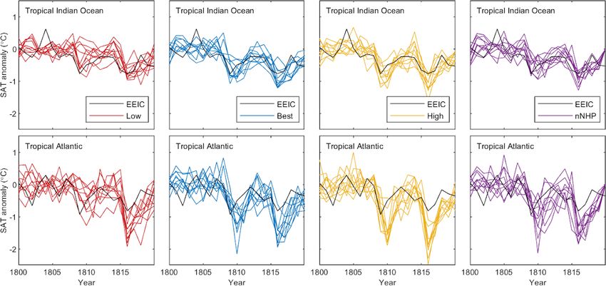
C. Timmreck et al.: The unidentified eruption of 1809: a climatic cold case                                                1461

et al. (2012) suggests a more modest cooling for the two early    anomalies, an indication for post-eruption “NH winter warm-
19th century eruptions of about 0.5 ◦ C (Fig. 2b). However,       ing”, are clearly visible in 1816/1817 in the second winter
the cooling is again found to be of comparable magnitude af-      after the Mt. Tambora eruption in 1815. Northern Europe
ter the 1809 and 1815 eruptions, and it therefore hints to a      shows the largest warm anomaly for all regions (about 3 ◦ C).
tropical location of the 1809 eruption, in agreement with the     Warm NH winter anomalies between 1.5 and 2 ◦ C are seen
ice-core data.                                                    in the winter 1809/1810 over northern and eastern Europe
   Tree-ring records capture volcanically forced summer           and over New England. Strong cooling, however, is found
cooling very well (e.g., Briffa et al., 1998; Hegerl et al.,      for the 1808/1809 winter in northern and central Europe. NH
2003; Schneider et al., 2015; Stoffel et al., 2015). However,     summer temperature anomalies are less variable than in win-
in the NH extratropics, SAT anomalies after 1809 are more         ter (Fig. 2d). A local distinct cooling is found in the “year
spatially and temporally complex compared to the typical          without summer” in 1816 over all regions except northern
post-eruption pattern with broad NH cooling. In tree-ring-        Europe, where it occurs a year later. The cooling after the
based temperature reconstructions for interior Alaska–Yukon       1809 eruption is not so pronounced as after the Mt. Tambora
(Briffa et al., 1994; Davi et al., 2003; Wilson et al., 2019),    eruption in 1815.
1810 is one of the coldest summers identified over recent            In general the station data support the spatial distribution
centuries. In earlier reconstructions of summer SAT in dif-       of the reconstructed near-surface temperature anomalies de-
ferent regions of the western United States (Schweingruber        rived from tree-ring data. They show a local minimum over
et al., 1991; Briffa et al., 1992), 1810 was shown to be the      northern, eastern, and southern Europe in NH summer 1810,
third-coldest summer in the British Columbia–Pacific North-       which does not appear over western and central Europe and
west region. Likewise, European tree-ring records show            New England. The warm anomalies of the order of 2 ◦ C,
cooling after 1809 (e.g., Briffa et al., 1992; Wilson et al.,     which are found in summer 1811 over eastern Europe, are not
2016). In contrast, tree-ring networks in certain regions such    captured by the N-TREND spatial reconstruction, although
as eastern Canada show a minimal response after 1809              some slight warming is seen in the data over eastern Poland,
(Gennaretti et al., 2018).                                        Belarus, and the Baltic states.
   Based on compilations of regional records, tree-ring-based
reconstructions of NH mean land summer SAT show a
                                                                  4     Results
large spread in hemispheric cooling after the 1809 erup-
tion (Fig. 2b), with anomalies of −0.87, −0.77, −0.21,            4.1    Simulations
and −0.15 ◦ C in 1810 for the N-TREND (S), NVOLC, N-
TREND (N), and SCH15 reconstructions, respectively. Al-           Firstly, we compare the simulated evolutions of monthly
though using the same dataset, the spatial N-TREND (S) and        mean near-surface (2 m) air temperature anomalies between
the nested N-TREND (N) reconstructions show quite differ-         the four experiments globally, in the tropics, and in the NH
ent behavior. In N-TREND (S), the nature of the spatial mul-      extratropics (Fig. 3). Ensemble-mean global-mean temper-
tiple regression modeling biases the input records to those       ature anomalies grow through 1809 and reach peak values
that correlate most strongly with local temperatures, which,      through 1810 in all experiments before decaying towards cli-
when available, are likely MXD data. In all four reconstruc-      matological values (Fig. 3a). Peak cooling reaches around
tions, NH temperature does not return to the climatological       1.0 ◦ C in the High experiment compared to 0.5 ◦ C in the Low
mean after an initial drop in 1810 but remains low or even        and nNHP experiments. Peak temperature anomalies across
exhibits a continued cooling trend until the Mt. Tambora          the experiments correlate with the magnitude of prescribed
eruption in 1815 (Schneider et al., 2015). The spatial vari-      AOD (Fig. 1a), and the responses are qualitatively consistent
ability of the reconstructed NH extratropical temperature re-     with expectations; the AOD for the Low and nNHP exper-
sponse to the 1809 eruption is illustrated in Fig. 2e, f, and g   iments, which is similar in magnitude to that from the ob-
based on the spatially resolved N-TREND (S) reconstruction        served 1991 Pinatubo eruption, leads to global-mean temper-
(Anchukaitis et al., 2017), displaying zonal oscillations con-    ature anomalies also similar to those observed after Pinatubo.
sistent with a “wave-2” structure that are especially evident     Global ensemble-mean near-surface temperature anomalies
in 1810 but already appreciable in 1809. This hemispheric         are close together in Low and nNHP over boreal summer
structure is in contrast with the relatively uniform cooling      but differ for boreal winter when the intrinsic variability is
seen in tree-ring records for Tambora (Fig. S3) and indeed for    higher. Low is the only experiment for which large-scale
many of the largest eruptions of the past millennium (Hartl-      temperatures return to within the 5th–95th percentile range
Meier et al., 2017).                                              of the control run before the Mt. Tambora eruption in 1815.
   Information about regional and seasonal mean NH tem-           Global-mean temperature anomalies of the other three exper-
perature anomalies in the early 19th century can be obtained      iments return only to within the 5th–95th percentile range of
from different station data across Europe and from New Eng-       unperturbed variability by 1815. As expected, almost no sig-
land (Fig. 2c, d). In NH winter the measurements reflect          nificant near-surface temperature anomalies are found for the
the high variability of local-scale weather (Fig. 2c). Warm       nNHP simulation in the NH extratropics except a few months

https://doi.org/10.5194/cp-17-1455-2021                                                      Clim. Past, 17, 1455–1482, 2021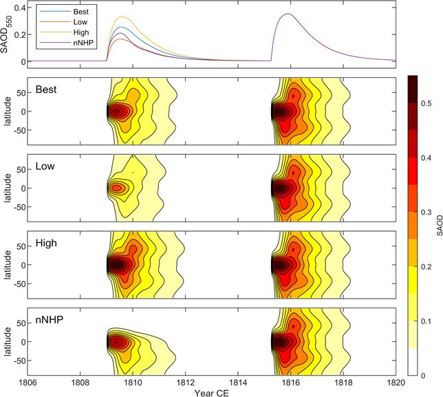
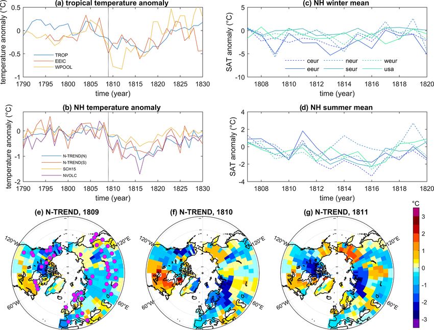
1462                                                   C. Timmreck et al.: The unidentified eruption of 1809: a climatic cold case

Figure 2. Observed and reconstructed temperature anomalies around the 1809 volcanic eruption. (a) Reconstructed tropical (30◦ N–30◦ S,
34◦ E–70◦ W) sea surface temperature (TROP; D’Arrigo et al., 2009), measured tropical marine surface air temperatures from EEIC ship
logs (Brohan et al., 2012), and Indo-Pacific warm pool data (D’Arrigo et al., 2006). (b) NH summer land temperatures from four tree-ring-
based reconstructions (Wilson et al., 2016, N-TREND (N); Anchukaitis et al., 2017, N-TREND (S); Guillet et al., 2017, NVOLC; Schneider
et al., 2015, SCH15). (c–d) Monthly mean NH winter (c) and summer (d) temperature anomalies (◦ C) from 53 station datasets averaged over
different European regions (central Europe, CEUR: 46.1–52.5◦ N, 6–17.8◦ E; eastern Europe, EEUR: 47–57◦ N, 18–32◦ E; northern Europe,
NEUR: 55–66◦ N, 10–31◦ E; southern Europe: 38–46◦ N, 7–13.5◦ E; western Europe, WEUR: 48.5–56◦ N, 6◦ W–6◦ O; and New England,
NENG: 41–44◦ N, 73–69◦ W). (e–g) Mean surface temperature anomalies ( ◦ C) for boreal summers of 1809 (e), 1810 (f), and 1811 (g) in
NH tree-ring data from N-TREND (S) (Anchukaitis et al., 2017). Pink dots in panel (e) illustrate the location of the tree-ring proxies used in
the N-TREND reconstructions.

in spring and autumn 1813 (Fig. 3b). The nNHP ensemble-                  Low exceeds the 5th–95th percentile range only for 2 years
mean values stay within the interquartile range of the con-              (Fig. 3c).
trol run but show a slight negative trend between 1809 and                  The ensemble distributions for the seasonal mean of win-
1815. The nNHP is also the only experiment in which the                  ter 1809/1810 and summer 1810 illustrate the differences be-
NH extratropical summer of 1814 is colder than the sum-                  tween the four experiments not only in the mean anomaly but
mer of 1809. Internal variability is relatively high in the NH           also for the ensemble spread (Fig. 3d–f). While, for example,
extratropics, in particular in NH winter, spanning more than             in summer 1810 the global and tropical ensemble means of
1.5 ◦ C. So, even the ensemble-mean near-surface tempera-                the Low and nNHP experiments are quite close, the ensem-
ture anomalies for the Best and High experiments almost                  ble spread is much larger in Low compared to nNHP. The
reach the 5th–95th percentile range of the control run in the            Low experiment generally has the largest ensemble spread
first post-volcanic winters. Peak cooling appears for all ex-            independent of season and hemispheric scale. The clearest
periments except nNHP in the summer 1810. In the tropics,                separation between the experiments appears in the NH ex-
the Best, High, and nNHP experiments are outside the 5th–                tratropics in summer 1810 (Fig. 3f), in line with Zanchettin
95th percentile range in the first 4 post-volcanic years, while          et al. (2019), who show with a k-means cluster analysis on

Clim. Past, 17, 1455–1482, 2021                                                               https://doi.org/10.5194/cp-17-1455-2021
C. Timmreck et al.: The unidentified eruption of 1809: a climatic cold case                                                            1463

Figure 3. Global, tropical, and extratropical temperature anomalies. Left: simulated ensemble-mean monthly anomalies of (a) global, (b) ex-
tratropical Northern Hemisphere, and (c) tropical averages of near-surface air temperature with respect to the pre-eruption (1800–1808) cli-
matology. All data are deseasonalized using the respective annual average cycle from the control run. Thick (thin) black dashed lines are the
5th–95th percentile intervals for signal occurrence in the control run for the ensemble mean (ensemble spread). Bottom bars indicate periods
when an ensemble member’s monthly mean temperature (color code as for the time series plots) is significantly different (p = 0.05) from
the control run according to the Mann–Whitney U test. Right: ensemble distributions (median as well as 25th–75th and 5th–95th percentile
ranges) of seasonal mean anomalies for the first post-eruption winter (1809–1810, DJF) and summer (1810, JJA) following the 1809 eruption
as well as for the pre-eruption period (1800–1808).

a large ensemble that forcing uncertainties can overwhelm                1810 as well as in the High and to a small extent also in the
initial condition spread in boreal summer.                               Best experiment in summer 1811. In nNHP no surface cool-
   A more detailed spatial distribution of the simulated tem-            ing is detectable over the NH extratropics in the first 4 years
poral evolution of post-volcanic surface temperature anoma-              after the eruption, consistent with the prescribed volcanic
lies is seen in the Hovmöller diagram in Fig. 4. It shows                forcing (see Fig. 1). However, a cooling anomaly is appar-
that in all four experiments a multiannual surface tempera-              ent around 60◦ N in summer 1813, which is seen in the zonal
ture response is found in the tropics (30◦ S–30◦ N). In the              mean over the ocean (Fig. S4) and likely due to decreased
inner tropics, the cooling disappears after 1.5 years in the             poleward ocean heat transport. Significant cooling south of
Low experiment and 2 to 3 years later in the Best, High, and             30◦ S appears only in austral spring 1809.
nNHP experiments. In the subtropics, a significant surface                  Figure 5 shows the spatial near-surface air temperature
cooling signal is found over the ocean until 1815 in Best and            anomalies for the first boreal winter (1809/1810) and the sec-
High, while over land no significant cooling appears in 1814             ond boreal summer (1810) after the 1809 eruption for the
(Fig. S4). A strong cooling signal is found in the NH extra-             four experiments. In general, the cooling is strongest over the
tropics in the Best, Low, and High experiments in summer                 NH continents in all experiments, revealing a strong cool-

https://doi.org/10.5194/cp-17-1455-2021                                                               Clim. Past, 17, 1455–1482, 2021
1464                                                C. Timmreck et al.: The unidentified eruption of 1809: a climatic cold case

Figure 4. Simulated ensemble-mean zonal-mean near-surface air temperature anomalies (◦ C) for the four MPI-ESM experiments. Only
anomalies exceeding 1 standard deviation of the control run are shown. Anomalies are calculated with respect to the pre-eruption (1800–
1808) climatology.

ing pattern over Alaska, Yukon, and the Northwest Territo-            shift of the Intertropical Convergence Zone (e.g., Haywood
ries in the first post-eruption winter. In the Best and High          et al., 2013; Pausata et al., 2020). This is clearly visible in
experiments, relatively strong cold anomalies are found over          the cold anomaly belt over the Sahel region in the asymmet-
the central Asian dry highland regions around 40◦ N from              ric forcing experiment nNHP. Significant warm anomalies
the Hindu Kush in the west to the Pacific, while the Low              are detectable in a small band that extends from the Caspian
and nNHP experiments show a small yet significant cooling             Sea in the west to Japan in the east. Cooling over the ocean
over India and southeastern China. In boreal winter a signif-         is weaker and mostly confined in the tropical belt between
icant warming is visible over Eurasia in all experiments ex-          30◦ S and 30◦ N. The High experiment is the only experi-
cept for Low, wherein warming anomalies are instead found             ment in which a significant El Niño-type anomaly is seen
over the polar ocean, and it is most pronounced in the High           over the Pacific Ocean in boreal summer 1810, while in the
experiment but also quite extensive in nNHP. Such an NH               other three experiments a slight but non-significant warming
winter warming pattern is known to be induced by atmo-                appears off the coast of South America. Looking at the rela-
spheric circulation changes (e.g., Wunderlich and Mitchell,           tive SST anomalies as calculated after Khodri et al. (2017),
2017; DallaSanta et al., 2019) and can occur in post-eruption         an El Niño-type anomaly is seen for all four scenarios in bo-
winters as a dynamic response to the enhanced stratospheric           real summer 1810, while in winter 1809/1810 a significant
aerosol layer when it displays a highly variable amplitude of         warming anomaly appears in the central tropical Pacific in
local anomalies (Shindell et al., 2004). Accordingly, in our          all experiments except the Best experiment (Fig. S5).
simulations the Eurasian winter warming pattern consists of              The substantial differences found in the post-eruption evo-
one or two areas with positive temperature anomalies cen-             lution of continental and subcontinental climates reflect the
tered over various locations between Fennoscandia and the             variety of climate responses produced by different combi-
Central Siberian Plateau in the different simulations. Signif-        nations of internal climate variability and forcing structure.
icant cooling, albeit of different strength, is found in the NH       In this regard, post-eruption anomalies of selected dominant
extratropics in boreal summer in the three symmetric forc-            modes of large-scale atmospheric circulation in the North-
ing experiments (Best, High, Low). However, while all of              ern Hemisphere and the tropics, including the Pacific–North
them show significant negative temperature anomalies over             American pattern, the North Atlantic Oscillation, the North
the North American continent with a local maximum over                Pacific Index, and the Southern Oscillation, yield a spread of
California and also cooling over Greenland, no significant            responses within individual ensembles that is often as large
anomalies are seen in the Low experiment over Fennoscan-              as the range of pre-eruption variability. Further, response dis-
dia. Except for some small regions (Finland, the Kola Penin-          tributions generated by different forcings in some cases do
sula, and western Alaska), no significant cooling is found in         not overlap (see Fig. S1).
nNHP in the NH extratropics in boreal summer. The spa-
tial distribution of the forcing can impact the latitudinal po-
sition of peak surface cooling, which in turn can lead to a

Clim. Past, 17, 1455–1482, 2021                                                          https://doi.org/10.5194/cp-17-1455-2021
C. Timmreck et al.: The unidentified eruption of 1809: a climatic cold case                                                           1465

Figure 5. Simulated ensemble-mean near-surface air temperature anomalies for the first winter (1809/1810) and the second summer (1810)
after the 1809 eruption for the four different MPI-ESM simulations. Shaded regions are significant at the 95 % confidence level according to
a t test. Anomalies are calculated with respect to the period 1800–1808.

4.2     Model–data comparison                                           et al., 2009) and the Indo-Pacific warm pool (D’Arrigo et al.,
                                                                        2006) in Fig. 6. The simulated ensemble-mean temperatures
4.2.1    Tropics                                                        (Fig. 6a) bracket the observed anomaly in the EEIC data in
A multiannual cooling signal is found in the MPI-ESM sim-               1809, with the observed value falling between the results of
ulations in the tropical region after the unidentified 1809             the Low and nNHP forcing experiments. In 1810–1812, the
eruption (Figs. 3 and 4). The same signature is detected in             cooling in the Best, High, and nNHP experiments is stronger
the English East India Company (EEIC) ship-based surface                than that observed, and therefore the results from the Low
air temperature anomaly annual means (Brohan et al., 2012)              experiment are generally the most consistent with the ship-
as well as in tropical SST reconstructions (TROP; D’Arrigo              borne measurements (Fig. 6a). When the model results are

https://doi.org/10.5194/cp-17-1455-2021                                                              Clim. Past, 17, 1455–1482, 2021
1466 C. Timmreck et al.: The unidentified eruption of 1809: a climatic cold case
sampled at the locations and times of the EEIC measure-
ments (Fig. S6), the mean negative temperature anomalies
in 1809 are 10 %–30 % smaller, with the Best, High, and
nNHP experiments all producing anomalies similar to that
of the EEIC measurements. For the 1810–1812 period, the
sampling makes little difference compared to the full trop-
ical average, with the Best, High, and nNHP experiments
all showing larger negative temperature anomalies than the
EEIC measurements. A comparison of TROP with our four
experiments reveals that all experiments lie within the 5th–
95th percentile interval of the TROP reconstruction, although
the reconstructed SST response appears to be dampened in
comparison to the model experiments (Fig. 6b). Although
the long-term trends of TROP and the model experiments
are in general agreement, the dampened post-volcanic cool-
ing could reflect autocorrelative biases in the proxies (Lücke
et al., 2019). Detailed scrutiny of high-resolution tropical
SST proxies and their potential biases to robustly reflect vol-
canically forced cooling has not been made in the same way
as has been performed for tree-ring archives over the last
decade (Anchukaitis et al., 2012; D’Arrigo et al., 2013; Esper
et al., 2015; Franke et al., 2013; Lücke et al., 2019). A simi-
lar behavior is found for the Indonesian warm pool (Fig. 6c).
However, in contrast to the whole tropics, the differences be- Figure 6. Comparison of tropical temperatures anomalies. Com-
tween the different forcing experiments are much smaller for parison of the MPI-ESM simulations with (a) tropical and annual
the warm pool region compared to the wider tropical regions, mean (30◦ N–30◦ S) surface air temperature from shipborne mea-
and the volcanic signal is more pronounced in the recon- surements of the English East India Company (EEIC; Brohan et al.,
structed SST, at least for the unidentified 1809 eruption. 2012), (b) annual mean tropical sea surface temperature (SST)
Tierney et al. (2015) provided coral-based reconstructions reconstruction (TROP; D’Arrigo et al., 2009) over the tropical
of tropical SSTs for four different ocean regions: the Indian Indo-Pacific (30◦ N–30◦ S, 34◦ E–70◦ W), and (c) seasonal mean
Ocean, the western and eastern Pacific, and the western At- (September–November) SST reconstruction (D’Arrigo et al., 2006)
lantic. Comparison of our four experiments with the coral- anomalies over the Indonesian warm pool (WP; 15◦ S–5◦ N, 110–
based reconstructions reveals quite different behavior and 160◦ E). The black line represents the observed or reconstructed
data in all panels, while the colored lines represent ensemble means
simulation–reconstruction agreement across the various re-
of the respective model simulations. The grey shaded regions in (b)
gions (Fig. 7). For the eastern Pacific region, the reconstruc- indicate the 95 % confidence interval of the reconstruction. Anoma-
tion and the MPI-ESM simulations are not inconsistent with lies are taken with respect to the years 1800 to 1808.
each other over the 1809 period, showing substantially high
variability (Fig. 7a) that reflects the influence of both ENSO
and volcanic cooling. A clear volcanic signal is therefore
found in the four experiments only for the Mt. Tambora erup- In the reconstruction, the Indian Ocean is the only region that
tion, while for the 1809 eruption, the High and Best experi- displays a peak cold anomaly after the Mt. Tambora eruption,
ments show a distinct cooling in 1809 and nNHP in 1811. In but the magnitude of this cooling is comparable to an appar-
contrast to the eastern Pacific, variability in the western Pa- ent cooling in 1807. A clear reference to the Mt. Tambora
cific is rather small (Fig. 7b). In all four experiments a clear eruption is therefore difficult to establish. No large cooling
volcanic signal is visible in the simulated ensemble-mean is found in the coral data after 1809 over the Indian Ocean
SST anomaly after the 1809 eruption and the Mt. Tambora (Fig. 7d).
eruption, whereas only a weak signal appears for both erup- Instrumental measurements from the tropical region are
tions in the reconstruction. Interestingly, in the western At- sparse, and no continuous temperature record covering the
lantic, two distinct positive SST anomalies appear in the re- early 19th century exists. Figure 8 shows a comparison be-
constructions in the aftermath of the unidentified 1809 and tween the model simulations and ship-based surface air tem-
the Mt. Tambora eruption, while the MPI-ESM simulations perature measurements from the tropical Atlantic and Indian
show cooling (Fig. 7c). Reasons for the anticorrelated behav- oceans. For each ocean basin, the model output is sampled at
ior are not obvious per se and may be related to changes in the locations and times of the ship measurements. For the In-
either ocean circulation or climate factors other than SST that dian Ocean, observed temperature anomalies after 1809 are
influence the coral record, such as salinity and precipitation. within the model ensemble spread of all the model ensem-
Clim. Past, 17, 1455–1482, 2021 https://doi.org/10.5194/cp-17-1455-2021C. Timmreck et al.: The unidentified eruption of 1809: a climatic cold case 1467 Figure 7. Coral–SST comparison. Comparison of reconstructed tropical annual mean SST (Tierney et al., 2015) with the MPI-ESM ex- periments over the (a) eastern Pacific (10◦ N–10◦ S, 175◦ E–85◦ W), (b) western Pacific (25◦ N–25◦ S, 110–155◦ E), (c) western Atlantic (15–30◦ N, 60–90◦ W), and (d) Indian (20◦ N–15◦ S, 40–100◦ E) oceans. Black solid line: SST reconstruction; colored lines: ensemble means of the model simulations. Anomalies are taken with respect to the years 1800 to 1808. The squares on the bottom of each panel indicate years when the observation lies outside the simulated ensemble range (color code as for the ensemble mean). Figure 8. Annual mean surface air temperature anomalies from shipborne measurements of the English East India Company (EEIC) (Brohan et al., 2012) over the tropical Indian and Atlantic oceans (black line) compared to similarly sampled model simulations from the Low, Best, High, and nNHP forcing ensembles as labeled. Anomalies are taken with respect to the years 1800 to 1808. https://doi.org/10.5194/cp-17-1455-2021 Clim. Past, 17, 1455–1482, 2021
1468 C. Timmreck et al.: The unidentified eruption of 1809: a climatic cold case
bles. The model response in the Indian Ocean is quite vari- substantially between the different tree-ring reconstructions.
able for the Low forcing experiment, with some members In N-TREND (N) the evolution is a step-like temperature de-
showing no apparent cooling and others with cooling of up to crease with a first step in 1809, followed by a second one
0.9 ◦ C. Overall, observed Indian Ocean temperature anoma- in 1812 and persistent low values until 1816. Distinct peak
lies are on the lower edge of the Low ensemble. For the Best, cooling appears in NVOLC and N-TREND (S) in NH 1810,
High, and nNHP experiments, the simulated cooling over followed by a short recovery phase in 1811 and a drop in
the Indian Ocean is more consistent across individual sim- 1812, but while summer SAT anomalies stay constant in the
ulations, with the ensemble spread enveloping the observed NVOLC reconstruction, for N-TREND (S) they start to re-
temperature time series. While Low forcing is not incon- cover again after 1812. Schneider et al. (2015) show only a
sistent with the observed Indian ocean temperatures, Best, small cooling trend between 1809 and 1815. In their recon-
High, and nNHP appear more likely scenarios. In the tropi- struction, temperatures after the 1809 event did not return to
cal Atlantic, the observed cooling after the 1809 eruption is their climatological mean after the initial drop but remained
slightly stronger than for Mt. Tambora and slightly stronger low until the Mt. Tambora eruption in 1815. Compared to
than that in the Indian Ocean. The maximum observed cool- the reconstructions, the ESM simulations (High, Best, Low)
ing in 1809 is roughly within the spread of all the model en- show a very different temporal evolution with a relatively fast
sembles. However, while observed tropical Atlantic tempera- recovery after the 1809 eruption to near background condi-
ture anomalies are largest in 1809, the simulated cooling usu- tions, followed by a second cooling peak for the Mt. Tamb-
ally peaks in 1810. In 1810, the observed cooling is less than ora eruption starting in 1816. In the MPI-ESM simulations
simulated in the Best ensemble and smaller than all but one no cooling peak appears in the ensemble mean for the sum-
of the individual simulations in the High ensemble. Looking mer of 1812, in contrast to the tree-ring records. The nNHP is
at the years after the Mt. Tambora eruption, simulations and the only experiment which shows only a slight cooling trend
observations agree relatively well in the Indian Ocean, while between 1810 and 1815, appearing closer to Schneider et al.
in the Atlantic, the model simulations overestimate the post- (2015). Between 1813 and 1815, nNHP reveals similar tem-
Tambora cooling. Since satellite observations of the aerosol perature anomalies as the Best and High experiments, while
cloud from the 1991 eruption of Pinatubo show that aerosol the Low experiment shows less cooling than all other exper-
quickly spreads uniformly across the tropics, it is unlikely iments, which even disappears before the onset of the Tamb-
that aerosol forcing from the 1809 eruption would be sig- ora eruption.
nificantly different between the tropical Indian and Atlantic In Fig. 10, we analyze the spatial patterns of the percentiles
Ocean basins. Therefore, differences in temperature response of the model ensemble into which the reconstruction falls. If
in the model between the two regions seems more likely to the reconstruction lies in the upper range of the distribution
be related to model sensitivity, which might particularly be of ensemble members, the reconstructed temperature anoma-
linked to differences in ocean circulation and/or mixed layer lies are warmer than most simulations; i.e., the majority of
depth. simulations are colder than the reconstruction. The High en-
semble (Fig. 10a) is in many locations colder than the re-
4.2.2 Northern Hemisphere extratropics
constructions, but the reconstruction from central to north-
ern Europe lies mostly within the interquartile, i.e., the 25th–
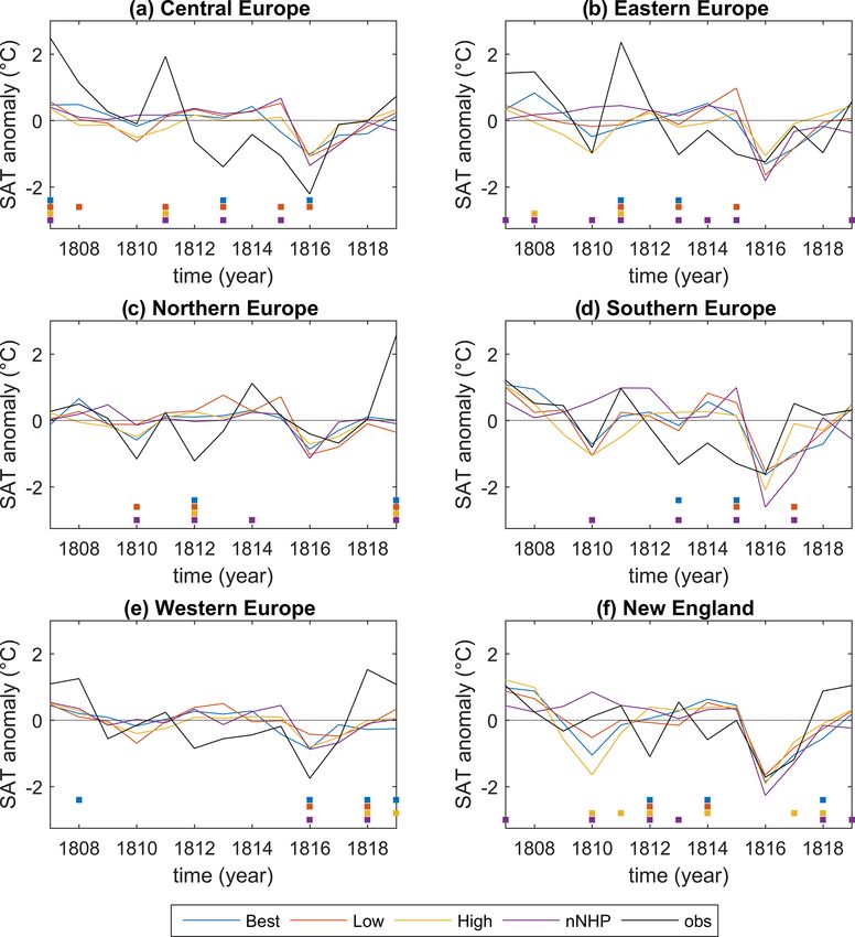
Figure 9 shows a comparison between the model experiments 75th percentile, range of the simulations. This behavior re-
with four NH summer land near-surface temperature recon- sults from the comparison of the variable local cooling in the
structions from tree-ring records, including the nested N- individual simulations with highly heterogeneous tempera-
TREND (N) (Wilson et al., 2016) and the spatial N-TREND ture anomalies in the reconstruction (Fig. 2). Only in a few
(S) reconstruction (Anchukaitis et al., 2017). To ensure com- regions (central Europe, western Russia, Alaska) are the sim-
parability between the reconstructions and the model re- ulated temperature anomalies much warmer and the recon-
sults, the data are expressed as anomalies with respect to structed one below the 25th percentile. The Best experiment
1800–1808. The High and Best experiments show signifi- (Fig. 10b) indicates a similar behavior as the High experi-
cantly larger cooling than the reconstructions and are out- ment albeit with more regions where the reconstruction lies
side the 95 % confidence interval of the N-TREND (N) re- within the interquartile range of the simulations, e.g., along
construction. Simulated SAT anomalies in nNHP are gener- the west coast of North America. Low (Fig. 10c) and nNHP
ally smaller than the reconstructions between 1809 and 1815. (Fig. 10d) are the experiments with the best agreement be-
The best agreement between the ESM simulations and the tween the simulated and the reconstructed surface tempera-
data after the 1809 eruption is found for the Low experiment. ture anomalies. The nNHP is the experiment in which, com-
In NH summer 1810 and 1811, the Low experiment matches pared to the other model experiments, the reconstruction in
the reconstructed temperature anomalies from the NVOLC most locations is within the interquartile range of the sim-
(Guillet et al., 2017) and N-TREND (S) records quite well. ulations and which has the lowest number of locations for
Interestingly, the devil really is in the detail. Despite the data which the reconstruction is considered an outlier compared
richness of this period, the temporal evolution (trend) differs to the simulation ensemble. Overall, the N-TREND (S) re-
Clim. Past, 17, 1455–1482, 2021 https://doi.org/10.5194/cp-17-1455-2021You can also read