353 Learning on the Job and the Cost of Business Cycles - SVERIGES RIKSBANK WORKING PAPER SERIES
←
→
Page content transcription
If your browser does not render page correctly, please read the page content below
SVERIGES RIKSBANK
 WORKING PAPER SERIES                  353

Learning on the Job and the
Cost of Business Cycles

Karl Walentin and Andreas Westermark

March 2018 (Updated January 2021)
WORKING PAPERS ARE OBTAINABLE FROM

                                  www.riksbank.se/en/research
                            Sveriges Riksbank • SE-103 37 Stockholm
                                 Fax international: +46 8 21 05 31
                             Telephone international: +46 8 787 00 00

                     The Working Paper series presents reports on matters in
                    the sphere of activities of the Riksbank that are considered
                                to be of interest to a wider public.
                   The papers are to be regarded as reports on ongoing studies
                      and the authors will be pleased to receive comments.

The opinions expressed in this article are the sole responsibility of the author(s) and should not be
                   interpreted as reflecting the views of Sveriges Riksbank.
Learning on the Job and the Cost of Business Cycles
Karl Walentinyand Andreas Westermarkz
Sveriges Rikbank Working Paper Series
No. 353
January 2021
Abstract
We show that business cycles reduce welfare through a decrease in the average level of employ-
ment in a labor market search model with learning on-the-job and skill loss during unemployment.
Empirically, unemployment and the job …nding rate are negatively correlated. Since new jobs are
the product of these two, business cycles imply that fewer news jobs are created and employment
falls. Learning on-the-job implies that the decrease in employment reduces aggregate human cap-
ital. This reduces the incentives to post vacancies, further decreasing employment and human
capital. We quantify this mechanism and …nd large output and welfare costs of business cycles.
Keywords: Search and matching, labor market, human capital, skill loss, stabilization policy.
JEL classi…cation: E32, J64.
We are deeply indebted to Virgiliu Midrigan (the editor) and three anonymous referees as well as Axel Gottfries and
Espen Moen and our discussants Marek Ignaszak, Tom Krebs and Oskari Vähämaa for detailed feedback on this paper.
We are also grateful to Olivier Blanchard, Tobias Broer, Carlos Carillo-Tudela, Melvyn Coles, Mike Elsby, Shigeru Fujita,
Jordi Galí, Christopher Huckfeldt, Gregor Jarosch, Per Krusell, Lien Laureys, Jeremy Lise, Kurt Mitman, Fabien Postel-
Vinay, Morten Ravn, Jean-Marc Robin, Richard Rogerson, Larry Summers, and conference and seminar participants at
Bank of England, Barcelona GSE Summer Forum (SaM), Board of Governors, CEF (Bordeaux), Conference on Markets
with Search Frictions, EEA (Lisbon), Essex Search and Matching Workshop, Georgetown University, Greater Stockholm
Macro Group, Labor Markets and Macroeconomics Workshop in Nuremberg, National Bank of Poland, Nordic Data
Meetings, Normac, NYU Alumni Conference, Royal Economic Society Annual Meeting (Bristol), Sciences Po, 22nd T2M
conference, UCLS (advisory board meeting), Uppsala University and University of Cambridge for useful comments. We
thank SNIC, the National Supercomputer Centre at Linköping University and the High Performance Computing Center
North for computational resources. The opinions expressed in this article are the sole responsibility of the authors and
should not be interpreted as re‡ecting the views of Sveriges Riksbank.
y
Research Division, Sveriges Riksbank, SE-103 37, Stockholm, Sweden. e-mail: karl.walentin@riksbank.se.
z
Research Division, Sveriges Riksbank, SE-103 37, Stockholm, Sweden. e-mail: andreas.westermark@riksbank.se.
11 Introduction
A major question in macroeconomics is how large the welfare costs of business cycles are. Since Lucas
(1987), it has been well established that the cost of aggregate consumption ‡uctuations is negligible.
Business cycles can induce welfare costs in other ways though, e.g., through their e¤ect on the cross-
sectional distribution of consumption (Imrohoro¼
glu, 1989, and many others). Furthermore, business
cycles may a¤ect welfare negatively by reducing the average level of output, a view that has been
argued by DeLong and Summers (1989), Hassan and Mertens (2017) and Summers (2015). Another
strand of the literature highlights the e¤ect of human capital dynamics on macroeconomic ‡uctuations,
see e.g., Kehoe, Midrigan and Pastorino (2015) and Krebs and Sche¤el (2017).
Our paper adds to this literature by presenting a new mechanism that ampli…es how business cycles
reduce the level of output. We show that business cycles substantially reduce the level of employment,
output and welfare in a labor market search model with human capital dynamics. There are two
channels through which business cycles reduce employment, and they constitute the initial step in
the main mechanism of this paper. The …rst channel is as follows: Empirically the job …nding rate
and the unemployment rate are strongly negatively correlated (see e.g. Shimer, 2005). Since new
jobs are the product of these two, aggregate volatility implies that fewer new jobs are created and
employment decreases, all else equal. At an intuitive level, this happens because the job …nding rate
in general is high when unemployment is low and vice versa. The second channel is speci…c to the
search and matching framework and works through the job …nding rate. Speci…cally, given some weak
parameter restrictions, the job …nding rate is a concave function of TFP in the textbook version of
this type of model, which implies that business cycles reduce the average job …nding rate and, in turn,
further reduce employment.1 In other words, worker congestion increase in booms, in the sense that
the increase in the job …nding rate slows down as TFP increases. In appendix A.1, we formally derive
su¢ cient conditions for when business cycles reduce employment in the stylized model. In settings
with learning on-the-job and skill loss during unemployment, any resulting fall in employment from
these two initial channels implies that average human capital falls. This, in turn, reduces the incentives
to post vacancies, further reducing employment and so on in a vicious circle, thereby amplifying the
initial impact of aggregate volatility on employment. Thus, aggregate volatility substantially reduces
employment, human capital and output. This process, including the ampli…cation mechanism, is
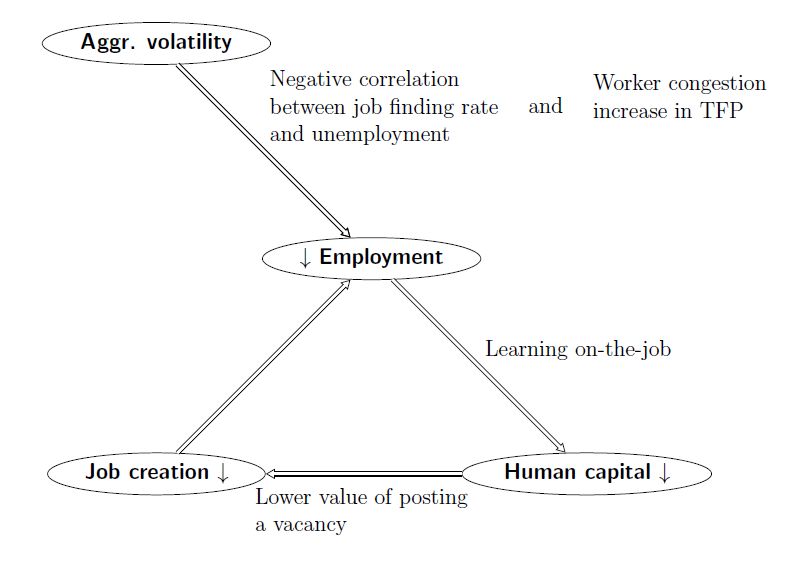
illustrated graphically in Figure 1. The size of the cost of business cycles generated by this mechanism
1
More generally, any convex cost (or concave bene…t or production function) in any cyclical variable tends to induce
a negative relationship between aggregate volatility and average consumption or employment. Prominent examples are
convex capital adjustment costs and convex vacancy posting costs, both of which are commonly used in the business
cycle literature.
2Figure 1: Illustration of main mechanism - how aggregate volatility reduces employment, human
capital and thereby output.
is accordingly largely determined by how sensitive the human capital distribution is to changes in
employment and how sensitive job creation is to changes in the human capital distribution. Since our
mechanism works through the average level of consumption, it is fundamentally di¤erent from most of
the cost of business cycles literature, which analyses the e¤ects of business cycles on welfare through
(aggregate or idiosyncratic) consumption volatility. Our ampli…cation mechanism also extends beyond
the cost of business cycles. For example, the e¤ect of a change in taxation or unemployment bene…ts
that a¤ects average employment will over time be ampli…ed by the human capital mechanism that we
have outlined.
We capture the mechanism described above that relates business cycles and the average level of
output using a search and matching framework with general human capital dynamics (learning on-the-
job and skill loss during unemployment). As argued above, an important determinant of the size of
the cost of business cycles is how sensitive job creation is to changes in the human capital distribution
of both unemployed and employed workers. Thus, we allow for on-the-job search to capture the e¤ect
of employed workers’ human capital on job creation. In addition, to allow for a ‡exible bargaining
framework in a context with on-the-job search, we use the bargaining protocol from Cahuc, Postel-
Vinay and Robin (2006), henceforth CPVR. In this framework workers can have positive bargaining
power and receive the value of their outside option plus a share of the value of the match above the
outside option. To allow for a positive bargaining power of workers is important since the level of
3bargaining power can have substantial e¤ects on welfare in search and matching models. We are not
aware of any previous model that uses the bargaining framework of CPVR in a setting with aggregate
uncertainty using global solution methods. In this paper, we propose and implement an algorithm for
solving models where workers with positive bargaining power that can search on-the-job meet …rms
with di¤erent levels of productivity. Thus, the paper also makes a methodological contribution. In
our mind, our solution algorithm is useful for future research where heterogeneity in the labor market
interacts with the business cycle.
The main purpose of our exercise is to provide a credible quanti…cation of the cost of business
cycles through the mechanism we have sketched above. One key determinant of this cost is the speed
of human capital accumulation when employed compared to the skill loss during unemployment. We
estimate the human capital gains when employed by matching the empirical “return to experience”
(wage pro…le of employed workers) reported by Buchinsky et al. (2010). The model is calibrated
by matching the return to experience and other relevant moments, including volatility of GDP and
unemployment, standard worker ‡ow moments and the degree of wage dispersion. We then compute
the cost of business cycles by comparing the equilibrium for our full model to the equilibrium from
the same model, but without aggregate volatility. We …nd that business cycles reduce steady state
employment, GDP and welfare by substantial amounts. In particular, eliminating aggregate volatility
increases welfare (GDP) by 0:70-1:68 percent (1:55 percent), depending on the interpretation of the ‡ow
value of unemployment. These are fairly large e¤ects, relative to the cost of aggregate consumption
volatility as in, e.g., Lucas (1987). Accounting for the transition dynamics, the welfare gains of
eliminating business cycles are somewhat smaller, 0:37-1:28 percent. Human capital dynamics are
pivotal for the results - if we disable them in our model, the implied employment, GDP and, in
particular, welfare losses from business cycles are substantially smaller. Note that, since we assume
risk neutral agents and hence abstract from, e.g., the direct welfare costs of consumption volatility, we
do not capture the full welfare cost of business cycles and our results can accordingly be interpreted
as a lower bound for these costs.
An important fact regarding the unemployment rate is that it varies across workers, where workers
with low human capital tend to have higher unemployment rates. In our model, we are able to capture
this fact using heterogeneity in match-speci…c productivity, which induces lower job …nding rates and
higher separation rates for workers with low human capital. This tends to worsen the composition
of the unemployment pool and implies that a worsening of the human capital distribution has strong
e¤ects on job creation. Speci…cally, workers with low human capital can meet …rms whose match
productivity imply a negative surplus. In addition, matches that are formed when the worker has low
4human capital, face an elevated risk of separating in the next downturn. Hence, expected surplus (over
match productivity) when hiring workers with low human capital is low. Furthermore, for workers
with a higher level of human capital, fewer meetings have negative surplus and future separation rates
are lower. Since the value of a new match depends on the human capital of workers, a reduction in the
human capital among the unemployed have large e¤ects on the incentives for …rms to post vacancies.
This leads to substantial e¤ects on job creation, unemployment and welfare. In models with learning
on-the-job but without match-speci…c productivity, a worsening of the human capital distribution has
no e¤ect on the job …nding rates and job separations through variations in these across human capital,
leading to substantially smaller e¤ects on job creation, unemployment and welfare. Speci…cally, using
a textbook search and matching model, Jung and Kuester (2011) …nd e¤ects that are an order of
magnitude smaller than in our paper.2
There is indicative empirical support for the relationship between aggregate volatility, unemploy-
ment and output implied by our model. Hairault et al. (2010) uses data for 20 OECD countries for
the period 1982-2003 and …nd signi…cant positive e¤ects of TFP volatility on average unemployment.
There is also ample evidence of a signi…cant negative relationship between volatility of output and
the average growth rate of output, see e.g., Ramey and Ramey (1995) and Luo et al. (2019). Direct
evidence of human capital dynamics, in the form of e¤ects on measurable skills, is documented by
Edin and Gustavsson (2008). They …nd sizeable skill loss e¤ects of unemployment. Additional indi-
rect evidence is provided by Schmieder, von Wachter and Bender (2016) who estimate a substantial
casual e¤ect on the re-employment wage of an additional month of unemployment, also indicating
considerable loss of human capital. There is also evidence that labor market conditions a¤ect the
future “employability”of workers. Yagan (2019) establishes a strong link between local shocks to em-
ployment growth during the Great Recession, 2007-2009, and the 2015 employment rates of workers
exposed to these shocks and argues that this link is due to depreciation of general human capital
during non-employment spells.
There are a number of papers analyzing related issues in a search and matching labor-market
setting. Dupraz, Nakamura and Steinsson (2019) use a model with downward nominal wage rigidities
to analyze the e¤ects of varying the in‡ation target on unemployment, output and welfare in a business
cycle setting. The e¤ects of business cycles on average unemployment and output can be large if the
in‡ation target is low, due to the inability of real wages to fall and thereby clear the market in
response to contractionary shocks. Den Haan and Sedlacek (2014) quantify the cost of business cycles
2
Hairault et al. (2010) also analyze a model with neither learning on-the-job nor match-speci…c productivity and …nd
e¤ects substantially smaller than ours.
5in a setting where an agency problem generates ine¢ cient job separations in downturns, thereby
reducing average employment and GDP. Our framework does not include any such agency problem
and is bilaterally e¢ cient. Furthermore, our model shares mechanisms with a number of papers that
analyze earnings losses from job displacement (Burdett, Carrillo-Tudela and Coles, 2020, Huckfeldt,
2016, Jarosch, 2015, Jung and Kuhn, 2019, and Krolikowski, 2017). Finally, Laureys (2014) analyzes
the e¤ects of skill loss in a business cycle setting using a linear framework.
The paper is outlined as follows. Section 2 presents the model, Section 3 documents the calibration
and Section 4 provides the quantitative results. Finally, Section 5 concludes.
2 Model
We set up a business cycle model with a search and matching labor market and human capital
dynamics. We allow for on-the-job search to capture the direct e¤ect of employed workers’ human
capital on vacancy postings. The basic building blocks of our model are similar to Lise and Robin
(2017), henceforth LR, except for the wage bargaining where we follow CPVR.3 This wage setting
framework implies that workers get the value of their outside option plus a share , re‡ecting their
bargaining strength, of the value of the match above the outside option. When a worker is hired out
of unemployment the outside option is the value of unemployment. If instead an employed worker
receives a poaching o¤er from another …rm, the outside option is the value of the second-best match.
In terms of human capital dynamics, the model is in the tradition of Pissarides (1992) and
Ljungqvist and Sargent (1998). As in these papers, we model general human capital as stemming
from learning on-the-job and skill loss during unemployment. Worker human capital, denoted by x,
follows a stochastic process and 0 0
xe (x; x ) ( xu (x; x )) denote the Markov transition probability for
the worker’s human capital level while employed (unemployed).4 Firm match-speci…c productivity is
denoted by y.
To summarize the above aspects of our model, in any time period there is heterogeneity across
employed workers in terms of human capital x; match-speci…c productivity y and wage w. Unemployed
workers only di¤er in terms of their human capital.
3
Compared to LR, the features we add are i) positive bargaining power of workers, and ii) learning on-the-job as well
as skill loss during unemployment. A simpli…cation compared to LR is that in our model the match-speci…c productivity
y of a match is not known when a vacancy is posted.
4
Our human capital dynamics di¤er slightly from Ljungqvist and Sargent (1998, 2008) and Jung and Kuester’s (2011)
extension with human capital in that we do not assume a sudden loss of general human capital when a worker separates
from a job. These papers abstract from heterogeneity in match-speci…c productivity and therefore assume, as a short-cut,
that part of the human capital loss occurs when a worker is separated from a job. This reduces the dependence of the
human capital distribution on employment (or any endogenous variable in the model), especially if one only allows for
exogenous separations.
6Utility is linear in consumption and there is no physical capital. Each …rm employs (at most)
one worker, and output from a match is p (x; y; z) = xyz where z is an aggregate TFP shock with
Markov transition probability (z; z 0 ). Note that the assumption of risk neutral agents implies that
we abstract from, e.g., the direct welfare costs of consumption volatility. Thus, we do not capture the
full welfare cost of business cycles and our results only re‡ect one of several factors a¤ecting these
costs.
2.1 Timing
Let us start the detailed model description by providing an overview of the timing protocol. The
sequence of events within a period are as follows. First, the aggregate productivity shock z and the
idiosyncratic human capital shocks x are realized. Second, a fraction of workers die and are replaced
by newborn unemployed workers with human capital at the lowest possible level, x, as in Ljungqvist
and Sargent (1998). Third, separations into unemployment occur. Then, …rms post vacancies and
workers search for jobs. Finally, new matches are formed, wages are set and production takes place.
2.2 Separations
The ability of recently separated workers to search for jobs within the period, makes it convenient
to de…ne match values and match surplus both before and after the search phase has occurred, i.e.,
at the separation stage and the matching stage. The surplus of a match at the separation stage is
S s (x; y; z; ) where denotes the endogenous aggregate state. Matches with S s (x; y; z; ) < 0 are
endogenously dissolved. In addition, a fraction of matches are exogenously destroyed every period.
The stock of unemployed workers after separations when the aggregate productivity evolves from
z 1 to z is:
2
X
us (x; z) = 1 fx = xg + (1 )4 u (x 1; z 1) xu (x 1 ; x) (1)
x 1 2X
3
X X
+ (1 fS s (x; y; z; ) < 0g + 1 fS s (x; y; z; ) 0g) h (x 1 ; y; z 1 ) xe (x 1 ; x)5
y2Y x 1 2X
where 1 fg is the indicator function, u (h) is the distribution of unemployed (employed) workers at the
end of a period, X is the set of human capital states and Y is the set of match-speci…c productivities.
Here, the …rst term is the newborn workers and the remaining terms captures the evolution of the
surviving workers.
7The stock of matches of type (x; y) at this point is:
X
hs (x; y; z) = (1 ) (1 ) 1 fS s (x; y; z; ) 0g h (x 1 ; y; z 1 ) xe (x 1 ; x) : (2)
x 1 2X
2.3 Search and matching
An employed worker exerts search e¤ort s1 . The search e¤ort of unemployed workers is normalized to
unity. Accordingly, the aggregate amount of search e¤ort is:
X XX
L us (x; z) + s1 hs (x; y; z) : (3)
x2X x2X y2Y
Vacancy posting costs are linear and each vacancy posted incurs a cost of c0 . The free entry
condition for vacancy creation therefore implies:
c0 = qJ (z; ) (4)
where q is the probability of a …rm meeting a worker and J is the expected value of a new match for a
…rm, as de…ned below. Note that the match-speci…c productivity, y, is observed when the …rm meets
a worker after the vacancy has been posted.5
We assume the following Cobb-Douglas meeting function:
M min L! V 1 !
; L; V (5)
where V is the number of vacancies posted and ! is the matching function elasticity. The probability
of a …rm meeting a worker (assuming an interior solution) is:
M !
q= = ;
V
V
where L is labor market tightness. Together with the matching function (5), this implies that
equilibrium vacancy postings are determined by:
1
J (z; ) !
V =L : (6)
c0
5
This assumption substantially simpli…es the computation of the equilibrium.
8We can then write labor market tightness as a function of z and :
1
J (z; ) !
(z; ) = : (7)
c0
Finally, the probability that an unemployed worker meets a …rm (the job meeting rate) is, assuming
an interior solution:
M
f (z; ) = = (z; )1 !
: (8)
L
2.4 Values
A worker who is unemployed during the production phase receives a ‡ow payo¤ of b (x; z) representing
unemployment insurance, utility of leisure and value of home production.6 The value of unemployment
at the matching stage is:
B (x; z; ) = b (x; z) (9)
1 X X X
+ [ f z0; 0
B x0 ; z 0 ; 0
+ max S x0 ; y 0 ; z 0 ; 0
;0 g y0
1+r 0 0 0
x 2X z 2Z y 2Y
0 0
+ 1 f z; 0
B x ; z0; 0
] xu x; x0 z; z 0 ;
where r is the discount rate, Z is the set of aggregate productivity states, is the bargaining strength
of workers, S the surplus of a match (de…ned below) and g (y) is the probability density function (pdf)
of the productivity of newly created matches. Thus, B is the ‡ow payo¤ b plus the job meeting rate
f (z 0 ; 0) times the discounted value of a job tomorrow plus (1 f (z 0 ; 0 )) times the discounted value
of being unemployed tomorrow. The max operator ensures that only matches with positive surplus
are formed. Note that while a worker is unemployed his human capital (weakly) decreases from x to
x0 with probability 0
xu (x; x ).
The match value at the matching stage, using that the job meeting rate for employed workers is
s1 f (z 0 ; 0 ), can be written as follows:
1 X X
s
P (x; y; z; ) = p (x; y; z) + [(1 (1 ) IS 0) B x0 ; z 0 ; 0
+ (1 ) IS 0
1+r 0 0 x 2X z 2Z
X
f s1 f z 0 ; 0
P x0 ; y; z 0 ; 0
+ max P x0 ; y~0 ; z 0 ; 0
P x0 ; y; z 0 ; 0
;0 g y~0 (10)
y~0 2Y
+ 1 s1 f z 0 ; 0
P x0 ; y; z 0 ; 0
g] xe x; x0 z; z 0
where y~0 denotes the match quality of the poaching …rm and where the indicator for non-separation
6
Unemployment insurance is …nanced by lump-sum taxation on all workers.
9is:
IS 0 = 1 S s x0 ; y; z 0 ; 0
0 :
Here, B s is the value when unemployed and S s is the surplus of the match at the separation stage
as de…ned below. The …rst term in (10) is the ‡ow output, the second term the value when the
match separates tomorrow, the third term the value when receiving a poaching o¤er tomorrow and
the last term the value when not receiving a poaching o¤er tomorrow. Also note that, regardless of
what happens tomorrow, human capital while employed today increases from x to x0 with probability
0
xe (x; x ). Then, in term of surplus of a match, i.e., S = P B,
1 X X
s
S (x; y; z; ) = p (x; y; z) b (x; z) + (1 ) IS 0S x0 ; y; z 0 ; 0
xe x; x0 z; z 0
1+r 0 0 x 2X z 2Z
1 X X
+ B s x0 ; z 0 ; 0
xe x; x0 xu x; x0 z; z 0 : (11)
1+r 0 0 x 2X z 2Z
Since we allow for a positive bargaining power of workers, the values at the separation stage di¤er
from the values at the matching stage. In particular, at the separation stage, the value of search
includes the share of the surplus received when hired at the matching stage. Accordingly, the value
for an unemployed worker at the separation stage is:
B s (x; z; ) = (1 f (z; )) B (x; z; ) (12)
X
+ f (z; ) [B (x; z; ) + max fS (x; y~; z; ) ; 0g] g (~
y) :
y~2Y
The corresponding surplus of a match at the separation stage is:
X
S s (x; y; z; ) = S (x; y; z; ) + s1 f (z; ) [ max fS (x; y~; z; ) S (x; y; z; ) ; 0g] g (~
y ) (13)
y~2Y
X
f (z; ) [ max fS (x; y~; z; ) ; 0g] g (~
y) :
y~2Y
Recalling that workers receive a value corresponding to their outside option plus a share of the
surplus of the match, the expected value of a new match for a …rm is:
1 XX s
J (z; ) = u (x; z) max f(1 ) S (x; y; z; ) ; 0g g (y) (14)
L
x2X y2Y
1 XXX
+ s1 hs (x; y~; z) max f(1 ) (S (x; y; z; ) S (x; y~; z; )) ; 0g g (y) :
L
x2X y2Y y~2Y
The …rst term in (14) refers to expected surplus from recruiting out of the pool of unemployed (us ),
10and the second term refers to expected surplus from recruiting from the pool of employed workers
(hs ).
In the classical search and matching model, an increase in (steady state) employment decreases
the vacancy …lling rate through the matching function and hence reduces vacancy posting. The same
applies here; see (4). In our model, as can be seen from (14), there are two additional channels a¤ecting
job creation. First, an increase in employment leads to a larger fraction of new hires coming from
other …rms. For a given level of worker human capital, the surplus to the …rm of poaching workers
from other …rms is lower than from hiring unemployed workers, and hence this mechanism also reduces
the incentives to post vacancies. Second, and counteracting the …rst two e¤ects, a higher employment
level increases average human capital among both pools of workers the …rms hires from, which leads
to stronger incentives for vacancy posting. This last e¤ect is the ampli…cation mechanism sketched in
Figure 1.
Let us here mention a computational aspect of the model. Solving the model is non-trivial because
the surplus (11) depend on the probability of the worker receiving a job o¤er the next period. This,
in turn, depends on the next period’s labor market tightness. According to (7) next period’s tightness
is fully determined by the expected value of a new match to a …rm in the next period, i.e., J (z 0 ; 0 ).
As can be seen from (14), this depends on the distribution of unemployed workers across human
capital and the distribution of matches over human capital and match-speci…c productivity. Hence,
the endogenous aggregate state can be written as a function of L and the two terms within the
summations in (14). Thus, three moments fully capture the implications of this large-dimensional
object. We then use a Krusell and Smith (1998)-like algorithm to let these three moments summarize
and predict the labor market tightness, thereby enabling us to solve the model. For details on the
solution algorithm, see Appendix A.3. In Appendix A.3.4, we in addition document the numerical
accuracy of our algorithm and its implementation.
2.5 Distributional dynamics
For a new match to be formed, two conditions are required: the two parties must meet according to
the meeting function (5) and the match must be an improvement over the status quo (the current
match or unemployment). The unemployment distribution after matching accordingly is:
0 1
M X
u (x; z) = us (x; z) @1 1 fS (x; y; z; ) 0g g (y)A : (15)
L
y2Y
11The corresponding expression for the distribution of matches is:
M
h (x; y; z) = hs (x; y; z) + us (x; z) 1 fS (x; y; z; ) 0g g (y)
| L {z }
mass hired from unemployment
M X
hs (x; y; z) s1 1 fS (x; y~; z; ) > S (x; y; z; )g g (~
y)
L
y~2Y
| {z }
mass lost to more productive matches
M X s
+s1 h (x; y~; z) 1 fS (x; y; z; ) > S (x; y~; z; )g g (y) : (16)
L
y~2Y
| {z }
mass poached from less productive matches
Note that, from the term related to hiring from unemployment, the job …nding rates tend to be higher
for workers with higher human capital, x, as they tend to be employable (i.e., S (x; y; z; ) 0) by
a larger fraction of the potential employers. This is in line with the empirical evidence in Morchio
(2020).
2.6 Wage determination and worker values
Let W (w; x; y; z; ) denote the present value to a worker with human capital x in a match with
productivity y, wage w and aggregate productivity z. These worker values are determined according
to the bargaining protocol in CPVR and are detailed as follows. Denote the renegotiated wage by w0 .
Workers hired out of unemployment receive the wage w0 such that their value is equal to the value of
unemployment plus a share of the match surplus:
W w0 ; x; y; z; = B (x; z; ) + S (x; y; z; ) : (17)
For employed workers who have received a poaching o¤er, the bargaining protocol implies that
these workers receive a present value W (w0 ; x; y; z; ) equal to the value of the second-best match
that they have encountered during a spell of continuous employment plus a share of the di¤erence
in surplus between the best and second-best match. Formally, if a worker of type x employed at a
…rm of type y meets a …rm of type y~ then, if S (x; y; z; ) < S (x; y~; z; ), the worker switches to the
new …rm and gets the wage w0 satisfying
W w0 ; x; y~; z; = P (x; y; z; ) + [S (x; y~; z; ) S (x; y; z; )] : (18)
If, instead, S (x; y; z; ) S (x; y~; z; ), the worker remains in his current match and gets a wage
12w0 that satis…es:
W w0 ; x; y; z; = max fP (x; y~; z; ) + [S (x; y; z; ) S (x; y~; z; )] ; W (w; x; y; z; )g : (19)
Note that, in case the value at the current wage is higher than the one implied by the outside option,
the wage is unchanged.
Wages for workers who do not receive poaching o¤ers can also be rebargained, as aggregate or
idiosyncratic shocks might a¤ect the various values. First, if the wage is such that it implies a
worker value that is larger than the match value, then the match would break down unless there
is renegotiation. Hence, the wage is then set so that W (w0 ; x; y; z; ) = P (x; y; z; ). Second, if
the wage is such that the worker value is lower than B (x; z; ) + S (x; y; z; ), the worker can ask
for a renegotiation with unemployment as the outside option. Hence, the wage is then set so that
W (w0 ; x; y; z; ) = B (x; z; ) + S (x; y; z; ). Finally, the current wage w is unchanged when the
value W is in the bargaining set:
B (x; z; ) + S (x; y; z; ) 6 W (w; x; y; z; ) 6 P (x; y; z; ) : (20)
To solve for wages, we compute the value for a worker earning w today, given that future values are
(partially) determined by (17)-(20). An employed worker earning the wage w in the current period
faces four possibilities in the next period: i) staying employed and not meeting any new …rm, ii)
staying employed and receiving a successful poaching o¤er and switching jobs, iii) staying employed
and receiving an unsuccessful poaching o¤er (and staying in the old job) and iv) separating. Note
that, if the worker becomes separated in the next period the worker still has a chance to …nd a new
job within the period. Imposing an interior solution for M , M = L! V 1 ! and using the de…nition of
q, the probability of meeting a new …rm for an employed worker is s1 f (z 0 ; 0 ). Then, given the wage,
w, the worker value (at the matching stage) is:
1 X X
W (w; x; y; z; ) = w + [ 1 s0 f 1 s1 f z 0 ; 0 0
Wnp (21)
1+r 0 0 x 2X z 2Z
X
+s1 f z 0 ; 0 0
Iy~>y Wp;~
y >y + (1
0
Iy~>y ) Wp;~
y y g (~
y )g
y~2Y
0 1
X
+s0 @B x0 ; z 0 ; 0
+ f z0; 0
S x0 ; y 0 ; z 0 ; 0
g y0 A ] xe x; x0 z; z 0 ;
y 0 2Y
13where
s0 = 1 S x0 ; y; z 0 < 0 + 1 S x0 ; y; z 0 ; 0
0
0
Wnp = min P x0 ; y; z 0 ; 0
; max W w; x0 ; y; z 0 ; 0
; B x0 ; z 0 ; 0
+ S x0 ; y; z 0 ; 0
Iy~>y = 1 S x0 ; y~; z 0 ; 0
> S x0 ; y; z 0 ; 0
0 0 0 0
Wp;~
y >y = P x ; y; z ; + S x0 ; y~; z 0 ; 0
S x0 ; y; z 0 ; 0
0
Wp;~
y y = max P x0 ; y~; z 0 ; 0
+ S x0 ; y; z 0 ; 0
S x0 ; y~; z 0 ; 0
; W w; x0 ; y; z 0 ; 0
;
where s0 denotes separations, Wnp
0 the value when not receiving a poaching o¤er, I
y~>y a successful
0
poaching o¤er, Wp;~ 0
y >y the value of a successful poaching o¤er and Wp;~
y y the value of an unsuccessful
poaching o¤er.
2.7 Wage distribution
When determining the wage distribution, it follows from the description of the wage setting above
that the current wage of the worker is a state variable. The distribution of matches over w, x and y
after separations is:
X
hs;w (w; x; y; z) = (1 ) (1 ) 1 fS s (x; y; z; ) 0g hw (w; x 1 ; y; z 1 ) xe (x 1 ; x) : (22)
x 1 2X
Analogously to (16) in section 2.5, we de…ne hw (w; x; y; z), i.e., the distribution after matching and
wage rebargaining; see Appendix A.2.
3 Calibration
3.1 Distributions and shock processes
The log of the exogenous part of TFP, z; follows an AR(1) process approximated by a Markov chain.
The log of match productivity, g (y), is normally distributed and its mean value is normalized to
0:5. The number of gridpoints for x, y and z are 10, 8 and 5, respectively.7 The wage grid contains
15 points and is chosen separately for each parameter vector so as to only cover the relevant wage
interval.8 In constructing the grid for human capital, x, we, as e.g., Jarosch (2015), follow Ljungqvist
and Sargent (1998, 2008) in using an equal-spaced grid and in setting the ratio between the maximum
7
For z, we use Tauchen and Hussey’s (1991) discretization of AR(1) processes with optimal weights from Flodén
(2008). This algorithm has been shown by Flodén (2008) to also be accurate for processes with high persistence.
8
The coarseness of the wage grid is less restrictive than it seems, as we map each “o¤-the-grid” wage to the two
nearest grid points using the inverse of the distance to the grid point as weight. Furthermore, the wage grid has no
impact on the allocations in the model.
14and minimum value of x to 2.9 The structure of the transition matrices 0
xe (x; x ) and 0
xu (x; x )
for human capital also closely follows Ljungqvist and Sargent. Abstracting from the bounds, the
probability of an employed worker to increase his/her human capital by one gridpoint is xup and the
probability for an unemployed worker to decrease his/her human capital by one gridpoint is xdn . With
the reciprocal probabilities, the human capital of a worker is unchanged. Note that there is very little
direct evidence on the shape of human capital dynamics. However, Edin and Gustavsson (2008) …nd
that skill loss appears to be linear in time out-of-work, in line with the assumption above.
3.2 Calibration approach
The frequency of the model is monthly. We calibrate the model based on U.S. data. Parameters
whose values are well established in the literature or can be set based on model-independent empirical
evidence are set outside the model. Table 1 documents these parameter values and their sources.
Table 1: Parameters set outside the model
Explanation Value Source
! Matching function elasticity 0:5 Pissarides (2009)
Exogenous match separation rate 0:030 Fujita-Ramey (2009)
c0 Vacancy posting cost 0:06375 Fujita-Ramey (2012)
Retirement rate 1=(40 12) 40-year work-life
TFP shock persistence 0:960 Hagedorn-Manovskii
r Interest rate 1:051=12 1 Annual r of 5%
The meeting function elasticity, !, is set in line with the convention in the literature. The exogenous
match separation rate, , is set equal to the mean E2U transition rate reported by Fujita and Ramey
(2009), adjusted for workers …nding a new job the same month as they lost the old job.10 This
adjustment implies that the separation rate exceeds the E2U rate by a factor of 1/(1-job …nding rate).
By using Fujita and Ramey’s number for E2U transitions, which is 0.020, we control for the fact that
empirically, but not in our model, workers ‡ow in and out of the labor force. We set the vacancy
posting cost c0 along the lines for Fujita and Ramey (2012) who refer to evidence that vacancy costs
are 6.7 hours per week posted.11 We set the retirement (or death) rate to match an average work-life
of 40 years, as e.g. Huckfeldt (2016). To compute the persistence of the AR process for TFP, we
follow along the lines of Hagedorn and Manovskii (2008). Speci…cally, we simulate a monthly Markov
chain to match a quarterly autocorrelation of (HP-…ltered) log labor productivity of 0:765. Finally,
9
The range of x-values is between 0:5 and 1. We explore a wider support for the values of x in a robustness exercise
documented
10
in section 4.3.3.
This calibration approach for assumes that the average endogenous separation rate in our model is negligible. We
con…rm this ex post - it is merely 0:0036 at the monthly frequency, i.e., 10% of the total separation rate.
11
Fujita-Ramey note that 6.7 hours per week is equivalent to 0.17 of a work week. Considering a monthly frequency,
and assuming that vacancy posting costs are proportional to the time the vacancy is kept posted, this implies c0 =
0:17E (xyz) 0:17xyz = 0:06375 where x, y and z = 1 are the midpoints of the grids over x, y and z, respectively.
15we set r to yield an annualized interest rate of 5% as in LR. For simplicity, and in line with most
of the literature, the ‡ow payo¤ from unemployment is b (x; z) = b0 in our baseline calibration, i.e.,
invariant of aggregate productivity and human capital.
Table 2: Parameters obtained by moment-matching
Parameter Explanation Value Main identifying moment
Matching function productivity 0.474 U2E transition rate, mean
s1 Relative search intensity of employed 0.156 J2J transition rate, mean
xup Human capital gain, probability 0.0315 Return to experience
b0 Unemployment payo¤ 0.321 Unemployment, std.dev.
Bargaining strength of workers 0.733 Wage elasticity wrt prod.
y Match-speci…c productivity dispersion 0.122 Wage disp: Mean-min ratio
100 z TFP shock std.dev. 0.670 GDP, std.dev.
The remaining parameters of our model are calibrated jointly to match key …rst and second mo-
ments. Table 2 documents the 7 calibrated parameters and the 7 moments matched, including the
main identifying moment for each parameter. We minimize the squared percentage deviation between
model and data moments. Let us now motivate the choice of moments. Note …rst, that since we are
interested in the cost of business cycles from a mechanism driven by unemployment volatility, it is im-
portant to match GDP and unemployment volatility. Turning to identi…cation, the model parameters
are jointly estimated, but some moments are more informative about certain parameters. The mean
transition rate from unemployment to employment is informative about the matching function produc-
tivity : The job-to-job transition rate is informative about the relative search intensity of employed
workers s1 . Return to experience, measured as the average percentage wage increase while employed,
is informative about on-the-job accumulation of human capital, xup .12 Unemployment volatility is in-
formative about the unemployment payo¤ parameter, b0 . As pointed out by Hagedorn and Manovskii
(2008), wage elasticity with respect to labor productivity is informative regarding worker bargaining
strength, . Wage dispersion is informative about the dispersion of match-speci…c productivity of
new vacancies, y. Finally, the volatility of GDP and unemployment are both informative about the
standard deviation of the aggregate productivity process.
Let us comment on the cross-sectional data we use. The relevant measure of wage dispersion for
our model is “residual” wage dispersion, i.e., controlling for heterogeneity not present in the model,
12
As in Jarosch (2015), we impose a relationship between xup and xdn such that the number of increases in human
capital roughly equals the number of decreases to minimize bunching at end-points of the human capital grid X. In
particular, letting utot denote the (implicitly, through the mean values of E2U and U2E) targeted value of unemployment,
we impose (1 ) xup 1 utot x = (1 ) xdn utot x + (x x) where x is the distance between two gridpoints
and x represents average human capital for dying workers. For computational reasons, we set x to the midpoint of the
grid. Furthermore x is the lower bound of the grid, representing the human capital of newly born workers. This implies
1 utot
xdn = xup 1 (1 [x x]
utot ) x utot
.
16Table 3: Data moments and matched model moments
Moment Data source Target value (data) Model value
U2E transition rate, mean Fujita-Ramey (2009) 0.340 0.348
J2J transition rate, mean Moscarini-Thompson 0.0320 0.0351
Unemployment, std.dev. BLS 1980-2010 0.107 0.117
GDP, std.dev. BEA 1980-2010 0.0136 0.0141
Wage disp: Mean-min ratio Hornstein et al. 1.50 1.59
Wage elasticity wrt productivity Hagedorn-Manovskii 0.449 0.454
Return to experience Buchinsky et al. 0.0548 0.0483
Notes: U2E and J2J transition rates are at a monthly frequency. Unemployment is a quarterly mean
of a monthly series. This variable, as well as GDP, labor productivity and aggregate wages (at the
quarterly frequency), have been logged and HP-…ltered with = 1; 600, both in the data and the
model.
such as education, sex, race etc. We take the mean-min ratio (capturing the minimum by the 10th
wage percentile) from Hornstein, Krusell and Violante (2007) as our measure of wage dispersion. We
use their preferred measure of 1.50, which is an average of their ratios from census, OES and PSID
data. Similarly to Kehoe et al. (2015) we use estimates from Buchinsky et al. (2010) to obtain the
“return to experience”. Speci…cally, from Buchinsky’s estimated coe¢ cients we obtain the marginal
return to experience of a worker in his third year of employment. We then match that to the wage
increase of workers in the model who works for three years for the same employer. We can thereby
keep the match-speci…c productivity …xed and obtain a clean measure of the e¤ect of human capital
on wages. We believe that their estimate of return to experience captures general human capital and
not …rm-speci…c human capital since Buchinsky et al. (2010) control for …rm-speci…c seniority.
4 Results
4.1 Targeted moments and the parameter estimates
The moment-matching exercise can be evaluated by comparing the last two columns in Table 3. The
model is able to …t most of these moments well, with less than 10 percent deviation for all but one
moment, wage dispersion.
It might appear surprising that we need to calibrate the volatility of (the exogenous part of) TFP,
but this is necessary since the model has internal ampli…cation and propagation of the exogenous
TFP shocks, as the distribution of human capital of workers, the productivity of matches and sorting
between workers and jobs varies over the cycle. All of this implies that measured TFP in our model
is a combination of exogenous TFP and endogenous propagation.13
13
One could potentially also calibrate the persistence of exogenous TFP jointly with the 7 parameters in Table 2 to
match e.g., the persistence of GDP. However, to reduce computational complexity we calibrate this parameter as outlined
17The above moment-matching exercise determines the 7 parameters in Table 2. The value for s1
in Table 2 indicates that employed workers meet prospective employers slightly less than 1=6th as
often as unemployed workers. We follow LR and report the replacement ratio for unemployed workers
as a fraction of the output of the best possible match. The value of b0 implies that this ratio is
0:643, averaged over the human capital values. Given this low value relative to e.g., Hagedorn and
Manovskii (2008), one might ask how our model is able to generate unemployment volatility that is
in line with the data. One reason is that due to heterogeneity in human capital and noting that the
unemployment payo¤ is invariant to the individual worker’s human capital, many workers that are
hired from unemployment have a relatively low productivity and hence a much higher replacement
rate than the average value of 0:643. Pro…ts for hiring …rms therefore tend to be low and hence
sensitive to variations in aggregate productivity. Thus, in settings with worker heterogeneity, a low
b0 can generate su¢ cient volatility in unemployment; a point also noted by Lise and Robin (2017).
Moreover, we …nd that worker bargaining strength is fairly high, 0:733, which is substantially above
Hagedorn and Manovskii (2008). Note that in our bargaining setup, wages in ongoing matches do not
change when they remain in the bargaining set. Thus, our model has wage rigidity in the spirit of Hall
(2005), which tends to drive the wage elasticity down, thereby yielding a higher estimate of . Finally,
in light of Hornstein, Krusell and Violante (2007), it may be surprising that we are able to match wage
dispersion. However, in contrast to their model, we allow for heterogeneity in both human capital and
match productivity, which enables us to match this moment well; see also Krolikowski (2019).
Given the centrality of human capital dynamics for our mechanism, we report and comment in
more detail on our estimates of the related parameters. The estimated Markov transition probability
(xup = 0:0315) imply that the expected monthly human capital increase for an employed worker is
0:164 percent, while the expected decrease when unemployed is 0:931 percent (for xdn = 0:366).14
We know of only one study with a direct measure in the literature of general human capital loss
while non-employed: Edin and Gustavsson (2008). They use a Swedish panel of individual level data
that includes test results on labor market-relevant general skills and information about employment
status between test dates. First, they …nd that time-out-of-work (compared to employment) implies
skill loss, signi…cant at the 1% level. Second, this skill loss appears to be linear in time out-of-work.
Third, the speed of skill loss is substantial; being out-of-work for a year implies losing skills equivalent
to 0.7 years of schooling.
Our values for human capital dynamics can be compared to estimates in models broadly similar to
above. Moreover, the persistence of GDP turns out to be fairly well matched in our calibration.
14
These values take into account the distribution of employed and unemployed workers across the human capital grid,
including the e¤ects of the bounds of the human capital grid.
18ours.15 Huckfeldt (2016) reports a 0:330 percent expected monthly human capital increase for workers
in skill-intensive jobs (0:220 percent in skill-neutral jobs). For unemployed workers Huckfeldt obtains
a gradual human capital decrease of 1:13 percent per month. Jarosch (2015) reports only the monthly
human capital Markov transitions probabilities: 0:0141 for employed and 0:131 for unemployed. In
Jarosch (2015), for an employed worker with the mid-point of human capital, this implies an expected
increase of 0:134 percent, and for the unemployed worker with the mid-point of human capital, it
implies a 1:25 percent decrease. To sum up this comparison to the literature, our human capital
accumulation for employed workers is in between the estimates of Huckfeldt (2016) and Jarosch (2015),
while for unemployed workers our value is slightly below their estimates.
4.2 Welfare measure
As is standard in the cost of business cycle literature since Lucas (1987), we report the fraction of
expected consumption agents are willing to forego to eliminate business cycles. In our model, the
linearity of utility in consumption makes welfare calculations straightforward, since then the ‡ow of
aggregate welfare is proportional to aggregate consumption.
To compute market consumption, we deduct vacancy posting costs from GDP. Note that one may
interpret the unemployment payo¤, b, in two ways, which has di¤erent welfare implications. In the
…rst interpretation, b is home production (or equivalently, from a welfare perspective, utility of leisure)
in which case the welfare relevant quantity is the sum of market consumption and the unemployment
payo¤. In the second interpretation, b is a pecuniary transfer with no direct e¤ect on aggregate utility.
We report results for both interpretations.16
4.3 Results for cost of business cycles
Our main exercise is to compute the consequences for welfare, GDP and employment of eliminating
aggregate volatility.17 As documented in Table 4, we …nd that in our model the elimination of ag-
15
First, there is an older empirical literature that attributes all wage loss when re-employed after an unemployment spell
to human capital loss and furthermore assumes that the wage equals marginal product of labor. This is not consistent
with our model so we can not use that literature for calibration or straight comparison. Second, some papers look at
the e¤ect on wages of an additional month of unemployment. The estimates in Neal (1995) imply that an additional
month of unemployment reduces the re-employment wage by 1:5%, which, under the assumption that the wage equals
marginal product of labor, is very much in line with the results here. Recent results by Schmieder et al. (2016) shows
that re-employment wages decrease by 0:8% per (additional) month unemployed. This is somewhat lower than our result,
but reasonably well in line if we think that there is some surplus sharing so that wages decrease less than human capital
for an additional month of unemployment. Under the assumption that the wage changes roughly in proportion to the
marginal product of labor, these two empirical studies bracket our results where the di¤erence in the change in human
capital for employed and unemployed workers is 0:931% + 0:164% = 1:095%.
16
There is also an intermediate case where b consists of both home production and transfers. The welfare gain of
eliminating aggregate volatility generated by our mechanism will then fall between these two cases.
17
We do this by setting exogenous productivity z constant and equal to the average in the stochastic simulation.
19gregate volatility increases steady state GDP by a substantial amount, 1:55 percent.18 This also has
consequences for steady state consumption and welfare, which increase by 0:70-1:68 percent depending
on the interpretation of the unemployment payo¤. As we will document below, these fairly large e¤ects
are due to the positive relationship between employment and human capital accumulation. Another
way to describe the consequences of removing aggregate volatility is through the e¤ects on the unem-
ployment rate which falls from 5:78 percentage points to 4:59 percentage points, corresponding to a
21 percent decrease.
Note that the assumption of risk neutral agents implies that only changes in levels of consumption
and employment matter for welfare. We thus abstract from the welfare costs of consumption volatility.
Our results capture only one of several factors that account for the total cost of business cycles and
can be viewed as a lower bound of this cost.
From an accounting perspective, the increase in GDP can be decomposed into the increase in
employment and the change in the average level of human capital of employed workers19 ;
T X X
X
1
E (x h ( )) = PT xh (x; y; zt ) :
t h (x; y; zt ) t x2X y2Y
As can be seen from Table 4, the increase in employment accounts for the bulk of the e¤ect on GDP. To
understand the e¤ects of human capital on employment, recall from (14) that job creation is a¤ected
by the human capital of both employed and unemployed workers. We …nd that the e¤ects through
the unemployed dominates. This is partly due to that the average levels of human capital for the
unemployed changes more;
T X
X
1
E (x u ( )) = PT xu (x; zt )
t u (x; zt ) t x2X
increases by 3:69 percent while E (x h ( )) increases by 0:30 percent. In addition, job creation is
much more sensitive to changes in human capital of the unemployed. Speci…cally, the elasticity of
J (z; ) with respect to E (x u ( )) is 1:49 while the elasticity of J (z; ) with respect to E (x h ( ))
is 0:27. It may be surprising that the change in E (x h ( )) is so moderate. However, the reason
is that the composition of the employed workers is a¤ected by the elimination of business cycles. In
18
This indicates that the Oi-Hartman-Abel e¤ect, where higher aggregate volatility increases output and employment,
is relatively unimportant; see Bloom et al. (2018). Moreover, the counteracting e¤ect emphasized in Laureys (2014)
working through compositional e¤ects on job creation does not seem to be important here.
19
Although negligible for our exercise, there are other factors than human capital a¤ecting average productivity.
Examples include the change in the average level of match-speci…c productivity, E (y h ( )), and the changed degree of
sorting between workers and …rms (as well as the covariation between any of these objects with the cycle).
20particular, the positive e¤ect that higher employment has on human capital is counteracted by the
tendency that, in the absence of aggregate volatility, …rms tend to accept workers with lower human
capital.
Table 4: Steady state e¤ects of eliminating business cycles (in percent)
Baseline No human capital dynamics
Welfare, b transfer, (GDP-vacancy cost) 1.68 0.56
Welfare, b home prod, (GDP-vacancy costs+b u) 0.70 0.03
GDP 1.55 0.53
Employment 1.26 0.71
E (x u ( )) 3.69 -
E (x h ( )) 0.29 -
In contrast to the simple model discussed in the introduction and Appendix A.1, both the job
creation margin and the separation margin can contribute to the cost of business cycles. One way of
quantifying their relative importance is to turn o¤ the job creation channel by counterfactually …xing
the job …nding rate to the value in the economy without aggregate volatility. The welfare gain of
eliminating business cycles is then 0.8 percent, which indicates that the job creation and separation
margins contribute roughly equally to the cost of business cycles.
4.3.1 The importance of human capital dynamics
Let us now quantify the importance of the change in the human capital distribution for the cost of
business cycles. To do this we perform a counterfactual exercise where we keep the human capital
distribution of the population (i.e., combining employed and unemployed workers) …xed when we
remove the aggregate volatility, thus shutting down the ampli…cation mechanism discussed in Figure
1 and in conjunction with equation (14). All other aspects of the computation is the same as in the
baseline exercise.20 The last column of Table 4 con…rms the importance of learning on-the-job, as
the version of our model without human capital dynamics implies that aggregate ‡uctuations have
substantially smaller e¤ect on welfare, GDP and employment. In particular, human capital is very
important for the welfare e¤ects of removing business cycles.
4.3.2 Accounting for the transition
We now compute the welfare consequences of eliminating aggregate volatility taking the transition
dynamics into account. As reported in Table 5, we …nd that in our model the elimination of aggregate
volatility when taking the transition into account increases welfare by 0:37-1:28 percent depending
20
We …x the human capital distribution by setting xup = xdn = = 0 and assume that it is given by the average
distribution in the baseline calibration with aggregate volatility. We also keep the incentives for job creation and
destruction unchanged, i.e., S and B are computed with the baseline human capital parameters.
21on the interpretation of the unemployment payo¤.21 We note that the welfare gains from removing
business cycles are lower when accounting for the transition than when simply comparing steady states.
The gains when accounting for the transition are lower for two reasons: discounting of the increased
future consumption and the extra vacancy posting costs related to the increase in employment along
the transition path. Note also that the transition to the non-stochastic steady state is reasonably fast;
the half-time of the transition of GDP is 3:8 years.
Table 5: Welfare e¤ects of eliminating business cycles (in percent)
Welfare, b transfer 1.28
Welfare, b home prod 0.37
4.3.3 Robustness
Two key determinants of the cost of business cycles in our model are i) how sensitive the human capital
distribution is to the change in (un)employment, and ii) how sensitive job creation is to changes in
the human capital distribution of unemployed and employed workers. An important factor a¤ecting
the sensitivity of the human capital distribution is the range of values that human capital can take
and two important factors a¤ecting the sensitivity of job creation to human capital is to what degree
the unemployment payo¤ depends on human capital and the bargaining strength of workers.
Thus, to judge the robustness of the results we re-calibrate it under alternative assumptions and
report the steady state welfare, GDP and employment cost of business cycles in Table 6. First, we
document what the cost of business cycles is when allowing for a wider range of values for human
capital. Recall that in our main calibration we have followed Ljungqvist and Sargent (1998, 2008) and
assumed that the ratio between the highest and the lowest human capital value is 2. We illustrate the
e¤ects of increasing this ratio by 20% to 2.4. We then re-calibrate the model by matching the same
moments as above in Table 3. We …nd that eliminating aggregate volatility leads to an increase of
welfare and GDP of 0:47-1:02 and 0:94 percent, respectively. In other words, compared to our baseline
calibration the cost of business cycles decrease somewhat, but the results seem not to be very sensitive
to the range.
Second, we vary the unemployment payo¤ by setting b (x; z) = b0 + b1 x. In our main calibration
we have chosen to impose b1 = 0 and calibrate b0 internally. One might wonder to what degree
21
We compute welfare when taking the transition into account in the following way. First, we simulate the economy
with aggregate volatility for several thousand periods. We then draw 1000 starting points for the transition from this
simulation and compute welfare in each of these starting points, given that productivity is constant at its mean value
for all future periods. Finally, we calculate the mean across the 1000 transitions.
22You can also read