Evaluation of 18 satellite- and model-based soil moisture products using in situ measurements from 826 sensors - HESS
←
→
Page content transcription
If your browser does not render page correctly, please read the page content below
Hydrol. Earth Syst. Sci., 25, 17–40, 2021
https://doi.org/10.5194/hess-25-17-2021
© Author(s) 2021. This work is distributed under
the Creative Commons Attribution 4.0 License.

Evaluation of 18 satellite- and model-based soil moisture products
using in situ measurements from 826 sensors
Hylke E. Beck1 , Ming Pan1 , Diego G. Miralles2 , Rolf H. Reichle3 , Wouter A. Dorigo4 , Sebastian Hahn4 ,
Justin Sheffield5 , Lanka Karthikeyan6 , Gianpaolo Balsamo7 , Robert M. Parinussa8 , Albert I. J. M. van Dijk9 ,
Jinyang Du10 , John S. Kimball10 , Noemi Vergopolan1 , and Eric F. Wood1
1 Department  of Civil and Environmental Engineering, Princeton University, Princeton, NJ, USA
2 Hydro-Climate  Extremes Lab (H-CEL), Ghent University, Ghent, Belgium
3 Global Modeling and Assimilation Office, NASA Goddard Space Flight Center, Greenbelt, MD, USA
4 Department of Geodesy and Geoinformation (GEO), Vienna University of Technology, Vienna, Austria
5 School of Geography and Environmental Science, University of Southampton, Southampton, United Kingdom
6 Centre of Studies in Resources Engineering, Indian Institute of Technology Bombay, Powai, Mumbai 400 076, India
7 European Centre for Medium-Range Weather Forecasts (ECMWF), Reading, UK
8 School of Geographic Sciences, Nanjing University of Information Science & Technology,

Nanjing, Jiangsu, People’s Republic of China
9 Fenner School of Environment and Society, Australian National University, Canberra, Australian Capital Territory, Australia
10 Numerical Terradynamic Simulation Group, University of Montana, Missoula, MT 59801, USA

Correspondence: Hylke E. Beck (hylke.beck@gmail.com)

Received: 24 April 2020 – Discussion started: 19 May 2020
Revised: 9 October 2020 – Accepted: 23 October 2020 – Published: 4 January 2021

Abstract. Information about the spatiotemporal variability       (SWI) smoothing filter resulted in improved performance
of soil moisture is critical for many purposes, including mon-   for all satellite products. The best-to-worst performance
itoring of hydrologic extremes, irrigation scheduling, and       ranking of the four single-sensor satellite products was
prediction of agricultural yields. We evaluated the temporal     SMAPL3ESWI , SMOSSWI , AMSR2SWI , and ASCATSWI ,
dynamics of 18 state-of-the-art (quasi-)global near-surface      with the L-band-based SMAPL3ESWI (median R of 0.72)
soil moisture products, including six based on satellite re-     outperforming the others at 50 % of the sites. Among the two
trievals, six based on models without satellite data assimila-   multi-sensor satellite products (MeMo and ESA-CCISWI ),
tion (referred to hereafter as “open-loop” models), and six      MeMo performed better on average (median R of 0.72 ver-
based on models that assimilate satellite soil moisture or       sus 0.67), probably due to the inclusion of SMAPL3ESWI .
brightness temperature data. Seven of the products are in-       The best-to-worst performance ranking of the six open-
troduced for the first time in this study: one multi-sensor      loop models was HBV-MSWEP, HBV-ERA5, ERA5-Land,
merged satellite product called MeMo (Merged soil Mois-          HBV-IMERG, VIC-PGF, and GLDAS-Noah. This ranking
ture) and six estimates from the HBV (Hydrologiska Byråns        largely reflects the quality of the precipitation forcing. HBV-
Vattenbalansavdelning) model with three precipitation inputs     MSWEP (median R of 0.78) performed best not just among
(ERA5, IMERG, and MSWEP) with and without assimila-              the open-loop models but among all products. The calibra-
tion of SMAPL3E satellite retrievals, respectively. As refer-    tion of HBV improved the median R by +0.12 on aver-
ence, we used in situ soil moisture measurements between         age compared to random parameters, highlighting the impor-
2015 and 2019 at 5 cm depth from 826 sensors, located pri-       tance of model calibration. The best-to-worst performance
marily in the USA and Europe. The 3-hourly Pearson cor-          ranking of the six models with satellite data assimilation
relation (R) was chosen as the primary performance met-          was HBV-MSWEP+SMAPL3E, HBV-ERA5+SMAPL3E,
ric. We found that application of the Soil Wetness Index         GLEAM, SMAPL4, HBV-IMERG+SMAPL3E, and ERA5.

Published by Copernicus Publications on behalf of the European Geosciences Union.
18                                     H. E. Beck et al.: Evaluation of 18 satellite- and model-based soil moisture products

The assimilation of SMAPL3E retrievals into HBV-IMERG              et al., 2015), the impact of model complexity on the accuracy
improved the median R by +0.06, suggesting that data as-           of soil moisture simulations (Fatichi et al., 2016), the degree
similation yields significant benefits at the global scale.        to which model deficiencies and precipitation data quality
                                                                   affect the added value of data assimilation (Xia et al., 2019),
                                                                   and the impact of smoothing filters such as the Soil Wetness
                                                                   Index (SWI; Wagner et al., 1999; Albergel et al., 2008) on
1    Introduction                                                  the performance ranking of products.
                                                                      Our main objective was to undertake a comprehensive
Accurate and timely information about soil moisture is valu-       evaluation of 18 state-of-the-art (quasi-)global near-surface
able for many purposes, including drought monitoring, wa-          soil moisture products in terms of their temporal dynamics
ter resources management, irrigation scheduling, prediction        (Sect. 2.1). Our secondary objective was to introduce seven
of vegetation dynamics and agricultural yields, forecasting        new soil moisture products (one multi-sensor merged satel-
floods and heat waves, and understanding climate change im-        lite product called MeMo introduced in Sect. 2.2 and six
pacts (Wagner et al., 2007; Vereecken et al., 2008; Ochsner        HBV model-based products introduced in Sect. 2.3 and 2.4).
et al., 2013; Dorigo and de Jeu, 2016; Brocca et al., 2017;        As reference for the evaluation, we used in situ soil moisture
Miralles et al., 2019; Tian et al., 2019; Karthikeyan et al.,      measurements between 2015 and 2019 from 826 sensors lo-
2020; Chawla et al., 2020). Over recent decades, numer-            cated primarily in the USA and Europe (Sect. 2.5). We aim to
ous soil moisture products suitable for these purposes have        shed light on the advantages and disadvantages of different
been developed, each with strengths and weaknesses (see Ta-        soil moisture products and on the merit of various techno-
ble 1 for a non-exhaustive overview). The products differ          logical and methodological innovations by addressing nine
in terms of design objective, spatiotemporal resolution and        key questions frequently faced by researchers and end users
coverage, data sources, algorithm, and latency. They can be        alike:
broadly classified into three major categories: (i) products
directly derived from active- or passive-microwave satellite           1. How do the ascending and descending retrievals per-
observations (Zhang and Zhou, 2016; Karthikeyan et al.,                   form (Sect. 3.1)?
2017b), (ii) hydrological or land surface models without
                                                                       2. What is the impact of the SWI smoothing filter
satellite data assimilation (referred to hereafter as open-loop
                                                                          (Sect. 3.2)?
models; Cammalleri et al., 2015; Bierkens, 2015; Kauffeldt
et al., 2016; Chen and Yuan, 2020), and (iii) hydrological or          3. What is the relative performance of the single-sensor
land surface models that assimilate soil moisture retrievals or           satellite products (Sect. 3.3)?
brightness temperature observations from microwave satel-
lites (Moradkhani, 2008; Pan et al., 2009; Pan and Wood,               4. How do the multi-sensor merged satellite products per-
2010; Liu et al., 2012; Lahoz and De Lannoy, 2014; Reichle                form (Sect. 3.4)?
et al., 2017).
   Numerous studies have evaluated these soil moisture prod-           5. What is the relative performance of the open-loop mod-
ucts using in situ soil moisture measurements (e.g., Jack-                els (Sect. 3.5)?
son et al., 2010; Bindlish et al., 2018), other independent            6. How do the models with satellite data assimilation per-
soil moisture products (e.g., Chen et al., 2018; Dong et al.,             form (Sect. 3.6)?
2019), remotely sensed vegetation greenness data (e.g., Tian
et al., 2019), or precipitation data (e.g., Crow et al., 2010;         7. What is the impact of model calibration (Sect. 3.7)?
Karthikeyan and Kumar, 2016). Pronounced differences in
spatiotemporal dynamics and accuracy were found among                  8. How do the major product categories compare
the products, even among those derived from the same data                 (Sect. 3.8)?
source. However, most studies evaluated only one specific
                                                                       9. To what extent are our results generalizable to other re-
product or a small subset (≤ 3) of the available products (e.g.,
                                                                          gions (Sect. 3.9)?
Martens et al., 2017; Liu et al., 2019; Zhang et al., 2019;
Tavakol et al., 2019). Additionally, many had a regional (sub-
continental) focus (e.g., Albergel et al., 2009; Gruhier et al.,   2     Data and methods
2010; Griesfeller et al., 2016), potentially leading to conclu-
sions with limited generalizability. Furthermore, several new      2.1    Soil moisture products
or recently reprocessed products have not been thoroughly
evaluated yet, such as ERA5 (Hersbach et al., 2020), ERA5-         We evaluated in total 18 near-surface soil moisture prod-
Land (C3S, 2019), and ESA-CCI V04.4 (Dorigo et al., 2017).         ucts, including six based on satellite observations, six based
There is also still uncertainty around, for example, the ef-       on open-loop models, and six based on models that as-
fectiveness of multi-sensor merging techniques (Petropoulos        similate satellite data (Table 1). We evaluated six products

Hydrol. Earth Syst. Sci., 25, 17–40, 2021                                               https://doi.org/10.5194/hess-25-17-2021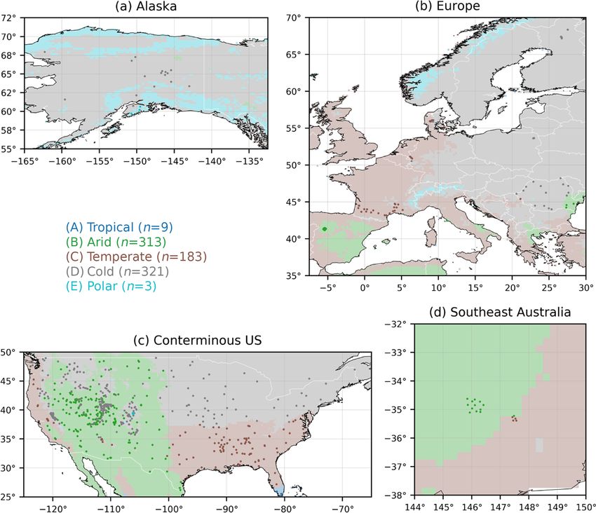
Table 1. The 18 soil moisture products evaluated in this study. For the single-sensor satellite products, the spatial sampling represents the footprint size and the temporal sampling the
average revisit time. Acronyms: A represents ascending, D represents descending, PMW represents passive microwave, AMW represents active microwave, P represents precipitation,
and DA represents data assimilation.
Acronym Details Spatial Temporal Temporal Latency Reference(s)
sampling sampling coverage
Satellite products
AMSR2a AMSR2/GCOM-W1 LPRM L3 V001 (soil_moisture_x); single-sensor PMW product; ∼ 47 km 1–3 d 2012–present ∼ 1.5 d Parinussa et al. (2015)
only D passes
ASCATa Combination of H115 and H116; single-sensor AMW product; A and D passes ∼ 30 km 1–2 d 2007–present 2–4 months Wagner et al. (2013),
H SAF (2019a, b)
SMAPL3Ea SPL3SMP_E.003 L3 Enhanced Radiometer EASE-Grid V3; single-sensor PMW ∼ 30 km 1–3 d 2015–present ∼2d Entekhabi et al. (2010a),
product; A and D passes Chan et al. (2018),
O’Neill et al. (2019)
https://doi.org/10.5194/hess-25-17-2021
SMOSa L2 User Data Product (MIR_SMUDP2) V650; single-sensor PMW product; A and D ∼ 40 km 1–3 d 2010–present ∼ 12 h Kerr et al. (2012)
passes
ESA-CCIa ESA-CCI SM V04.4 COMBINED; multi-sensor merged AMW- and PMW-based 0.25◦ Daily 1978–2018 About a year Dorigo et al. (2017),
product derived from AMSR2, ASCAT, and SMOS Gruber et al. (2019)
MeMo Multi-sensor merged PMW product derived from AMSR2, SMAPL3E, and SMOS with 0.1◦ 3-hourly 2015–present ∼ 12 h This study (Sect. 2.2)
SWI filter
Open-loop models (i.e., without data assimilation)
ERA5-Land Volumetric soil water layer 1 (0–7 cm); H-TESSEL model; forced with ERA5 P 0.1◦ Hourly 1979–2020 2–3 months C3S (2019)
(Hersbach et al., 2020)
GLDAS-Noah GLDAS_NOAH025_3H.2.1 (SoilMoi0_10cm_inst) forced with GPCP V1.3 Daily 0.25◦ 3-hourly 1948–2020 ∼ 4 months Rodell et al. (2004),
Analysis P (Huffman et al., 2001) Rui et al. (2020)
HBV-ERA5 HBV forced with ERA5 P (Hersbach et al., 2020) 0.28◦ 3-hourly 1979–2020 ∼6d This study (Sect. 2.3)
HBV-IMERG HBV forced with IMERGHHE V06 P (Huffman et al., 2014, 2018) 0.1◦ 3-hourly 2000–present ∼3h This study (Sect. 2.3)
HBV-MSWEP HBV forced with MSWEP V2.4 P (Beck et al., 2019b) 0.1◦ 3-hourly 2000–present ∼ 3 hb This study (Sect. 2.3)
H. E. Beck et al.: Evaluation of 18 satellite- and model-based soil moisture products
VIC-PGF Layer 1 (0–30 cm) of VIC forced with PGF (Sheffield et al., 2006) 0.25◦ Daily 1950–2016 Several years He et al. (2020)
Models with satellite data assimilation
ERA5 ECMWF ERA5-HRES reanalysis layer 1 (0–7 cm); ASCAT soil moisture DA 0.28◦ Hourly 1979–2020 ∼6d Hersbach et al. (2020)
GLEAM GLEAM V3.3a surface layer (0–10 cm); MSWEP V2.2 P forcing; ESA-CCI DA 0.25◦ Daily 1980–2018 6–12 months Martens et al. (2017)
HBV-ERA5+SMAPL3E HBV forced with ERA5 P ; SMAPL3E DA 0.1◦ 3-hourly 2015–2020 ∼6d This study (Sect. 2.4)
HBV-IMERG+SMAPL3E HBV forced with IMERG P ; SMAPL3E DA 0.1◦ 3-hourly 2015–present ∼2d This study (Sect. 2.4)
HBV-MSWEP+SMAPL3E HBV forced with MSWEP P ; SMAPL3E DA 0.1◦ 3-hourly 2015–present ∼2d This study (Sect. 2.4)
SMAPL4 SMAP L4 V4 surface layer (0–5 cm); NASA Catchment model forced with GEOS P 9 km 3-hourly 2015–present ∼2d Reichle et al. (2019b, a)
corrected using CPC Unified (Chen et al., 2008); SMAP brightness temperature DA
a We also evaluated versions of these products with Soil Wetness Index (SWI) filter (Wagner et al., 1999; Albergel et al., 2008) with the time lag constant T set to 5 d. b At a latency of hours, MSWEP does not include daily gauge
corrections and is therefore of lower quality. The data evaluated here have an effective latency of several days.
Hydrol. Earth Syst. Sci., 25, 17–40, 2021
19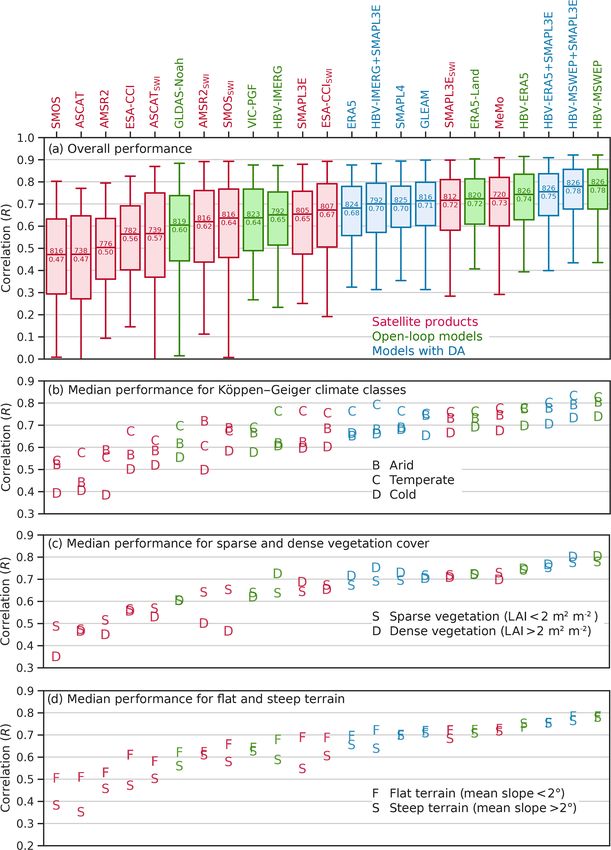
20                                            H. E. Beck et al.: Evaluation of 18 satellite- and model-based soil moisture products

per category, which was sufficient to compare the perfor-
mance among and within product categories and address
the questions posed in the introduction. We only considered
widely used products with (quasi-)global coverage, and we
attempted to keep the selection of products in each category
as diverse as possible. For example, we considered products
based on several major satellite missions used for global soil
moisture mapping (AMSR2, ASCAT, SMAP, and SMOS),
models of various type and complexity (with and without
calibration), different sources of precipitation data (satellites,
reanalyses, gauges, and combinations thereof), and various               Figure 1. To illustrate the SWI filter, SMAPL3E instantaneous vol-
data merging and assimilation techniques (with different in-             umetric soil moisture retrievals (from both ascending and descend-
                                                                         ing overpasses) and 3-hourly SMAPL3ESWI time series obtained
puts).
                                                                         by application of the SWI filter (with the time lag constant T set to
   The units differed among the products; some are provided
                                                                         5 d) for a 2-month period at 34.82◦ N, 89.44◦ W.
in volumetric water content (typically expressed in m3 m−3 ,
e.g., ERA5) and others in degree of saturation (typically
expressed in percent (%), e.g., ASCAT). We did not har-                     The vertical support is physically consistent with in situ
monize the units among the products, because the Pearson                 soil moisture measurements at 5 cm depth for most mod-
correlation coefficient – the performance metric used in the             els. The average depth of the soil layer (i.e., half the depth
current study (Sect. 2.6) – is insensitive to the units. Since           of the lower boundary) is 2.5 cm for SMAPL4, 3.5 cm for
the evaluation was performed at a 3-hourly resolution, we                ERA5 and ERA5-Land, 5 cm for GLEAM, 8.5 cm for HBV-
downscaled the two products with a daily temporal resolu-                ERA5, 6.6 cm for HBV-IMERG, 7.3 cm for HBV-MSWEP,
tion (VIC-PGF and GLEAM) to a 3-hourly resolution using                  and 15 cm for VIC-PGF (Tables 1 and S1). The soil layers
nearest-neighbor resampling (resulting in replication of the             of HBV may seem too deep, especially since they represent
daily value for all 3-hourly periods on each day). In contrast           conceptual “buckets” that can be fully filled with water, in
to the model products, the satellite products (with the excep-           contrast to the soil layers of the other models which addi-
tion of ASCAT) often do not provide retrievals when the soil             tionally consist of mineral and organic matter. However, the
is frozen or covered by snow (Fig. S1 in the Supplement).                soil layer depths of HBV were calibrated (see Sect. 2.3) and
To keep the evaluation consistent, we used ERA5 (Hersbach                are thus empirically consistent with in situ measurements at
et al., 2020) to discard the estimates of all 18 products when           5 cm depth.
the near-surface soil temperature of layer 1 (0–7 cm) was
< 4 ◦ C and/or the snow depth was > 1 mm.                                2.2   Merged soil Moisture (MeMo) product
   To deepen the vertical support of the superficial satellite
observations and suppress noise, we also evaluated 3-hourly              Merged soil Moisture (MeMo) is a new 3-hourly soil mois-
versions of the satellite products processed using the SWI               ture product derived by merging the soil moisture anomalies
exponential smoothing filter (Wagner et al., 1999; Albergel              of three single-sensor passive-microwave satellite products
et al., 2008). MeMo was not processed as it was derived from             with SWI filter (AMSR2SWI , SMAPL3ESWI , and SMOSSWI ;
SWI-filtered products. The SWI filter is defined according to            Table 1). MeMo was produced for 2015–2019 (the period
                                                                         with data for all three products) as follows:
                                   t−ti
                SMsat (ti )e−
           P
                                    T
                                                                           1. Three-hourly soil moisture time series of AMSR2SWI ,
            i
SWI(t) =                    t−ti          ,                      (1)          SMAPL3ESWI , SMOSSWI , the active-microwave satel-
                       e−
                  P
                             T
                                                                              lite product ASCATSWI , and the open-loop model HBV-
                   i
                                                                              MSWEP were normalized by subtracting the long-term
where SMsat (units depend on the product) is the soil mois-                   means and dividing by the long-term standard devia-
ture retrieval at time ti , T (d) represents the time lag constant,           tions of the respective products (calculated for the pe-
and t represents the 3-hourly time step. T was set to 5 d for                 riod of overlap).
all products, as the performance did not change markedly
                                                                           2. Three-hourly anomalies were calculated for the five
using different values, as also reported in previous studies
                                                                              products by subtracting their respective seasonal clima-
(Albergel et al., 2008; Beck et al., 2009; Ford et al., 2014;
                                                                              tologies. The seasonal climatology was calculated by
Pablos et al., 2018). Following Pellarin et al. (2006), SWI at
                                                                              taking the multi-year mean for each day of the year,
time t was only calculated if ≥ 1 retrievals were available in
                                                                              after which we applied a 30 d central moving mean to
the interval (t − T , t] and ≥ 3 retrievals were available in the
                                                                              eliminate noise. The moving mean was only calculated
interval [t − 3T , t − T ]. Figure 1 illustrates the filter for the
                                                                              if > 21 d with values were present in the 30 d window.
SMAPL3 product.
                                                                              Due to the large number of missing values in winter

Hydrol. Earth Syst. Sci., 25, 17–40, 2021                                                     https://doi.org/10.5194/hess-25-17-2021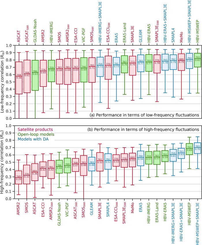
H. E. Beck et al.: Evaluation of 18 satellite- and model-based soil moisture products                                         21

      (Fig. S1), we were not able to compute the seasonality      hourly 0.1◦ resolution; Beck et al., 2017b, 2019b). For the
      and, in turn, the anomalies in winter for some satellite    ERA5 and IMERG datasets, we calculated 3-hourly precip-
      products.                                                   itation accumulations. Daily potential evaporation was esti-
                                                                  mated using the Hargreaves (1994) equation from daily min-
 3. Time-invariant merging weights for AMSR2SWI ,                 imum and maximum air temperature. The daily potential
    SMAPL3ESWI , and SMOSSWI were calculated using                evaporation data were downscaled to 3-hourly using nearest-
    extended triple collocation (McColl et al., 2014), a          neighbor resampling. Air temperature estimates were taken
    technique to estimate Pearson correlation coefficients        from ERA5. To improve the representation of mountainous
    (R) for independent products with respect to an un-           regions and ameliorate potential biases, the ERA5 air tem-
    known truth. The R values for the respective products         perature data were matched on a monthly climatological ba-
    were determined using the triplet consisting of the           sis using an additive (as opposed to multiplicative) approach
    product in question in combination with ASCAT and             to the comprehensive station-based WorldClim climatology
    HBV-MSWEP, which are independent from each other              (V2; 1 km resolution; Fick and Hijmans, 2017).
    and from the passive products. The R values were                 We calibrated the 7 relevant parameters of HBV us-
    only calculated if > 200 coincident anomalies were            ing in situ soil moisture measurements from 177 indepen-
    available. The weights were calculated by squaring the        dent sensors from the International Soil Moisture Network
    R values.                                                     (ISMN) archive (Sect. 2.5; Fig. S2). These sensors did not
 4. For each 3-hourly time step, we calculated the weighted       have enough measurements during the evaluation period
    mean of the available anomalies of AMSR2SWI ,                 (31 March 2015 to 16 September 2019) and thus were avail-
    SMAPL3ESWI , and SMOSSWI . If only one anomaly                able for an independent calibration exercise. The parameter
    was available, this value was used and no averaging           space was explored by generating N = 500 candidate pa-
    was performed. The climatology of SMAPL3E – the               rameter sets using Latin hypercube sampling (McKay et al.,
    best-performing product in our evaluation – was sub-          1979), which splits the parameter space up into N equal in-
    sequently added to the result, to yield the MeMo soil         tervals and generates parameter sets by sampling each inter-
    moisture estimates.                                           val once in a random manner. The model was subsequently
                                                                  run for all candidate parameter sets, after which we selected
2.3   HBV hydrological model                                      the parameter set with the best overall performance across the
                                                                  177 sites (Table S1). As objective function, we used the me-
Six new 3-hourly soil moisture products were produced using       dian Pearson correlation coefficient (R) calculated between
the Hydrologiska Byråns Vattenbalansavdelning (HBV) con-          3-hourly in situ and simulated soil moisture time series. To
ceptual hydrological model (Bergström, 1976, 1992) forced         avoid giving one of the precipitation datasets an unfair ad-
with three different precipitation datasets and with and with-    vantage, we recalibrated the model for each of the three pre-
out assimilation of SMAPL3E soil moisture estimates, re-          cipitation datasets (ERA5, IMERG, and MSWEP).
spectively (Table 1). HBV was selected because of its low
complexity, high agility, computational efficiency, and suc-      2.4   Soil moisture data assimilation
cessful application used in numerous studies spanning a wide
range of climate and physiographic conditions (e.g., Steele-
                                                                  Instantaneous soil moisture retrievals (without SWI filter)
Dunne et al., 2008; Driessen et al., 2010; Beck et al., 2013;
                                                                  from SMAPL3E (Table 1) were assimilated into the HBV
Vetter et al., 2015; Jódar et al., 2018). The model has 1 soil
                                                                  model forced with the three above-mentioned precipitation
moisture store, 2 groundwater stores, and 12 free parame-
                                                                  datasets (ERA5, IMERG, and MSWEP). Previous regional
ters. Among the 12 free parameters, 7 are relevant for sim-
                                                                  studies that successfully used HBV to assess the value of
ulating soil moisture as they pertain to the snow or soil rou-
                                                                  data assimilation include Parajka et al. (2006), Montero et al.
tines, while 5 are irrelevant for this study as they pertain to
                                                                  (2016), and Lü et al. (2016). We used the simple Newtonian
runoff generation or deep percolation. The soil moisture store
                                                                  nudging technique of Houser et al. (1998) that drives the soil
has two inputs (precipitation and snowmelt) and two out-
                                                                  moisture state of the model towards the satellite observations.
puts (evaporation and recharge). The model was run twice
                                                                  Nudging techniques are computationally efficient and easy to
for 2010–2019: the first time to initialize the soil moisture
                                                                  implement, and they have therefore been used in several stud-
store and the second time to obtain the final outputs.
                                                                  ies (e.g., Brocca et al., 2010b; Dharssi et al., 2011; Capecchi
   HBV requires time series of precipitation, potential evap-
                                                                  and Brocca, 2014; Laiolo et al., 2016; Cenci et al., 2016;
oration, and air temperature as input. For precipitation, we
                                                                  Martens et al., 2016). For each grid cell, the soil moisture
used three different datasets: (i) the reanalysis ERA5 (hourly
                                                                  state of the model was updated when a satellite observation
0.28◦ resolution; Hersbach et al., 2020); (ii) the satellite-
                                                                  was available according to
based IMERG dataset (Late Run V06; 30 min 0.1◦ reso-
lution; Huffman et al., 2014, 2018); and (iii) the gauge-,
                                                                  SM+           −                          −
                                                                                             sc
satellite-, and reanalysis-based MSWEP dataset (V2.4; 3-            mod (t) = SMmod (t) + kG SMsat (t) − SMmod (t) ,         (2)

https://doi.org/10.5194/hess-25-17-2021                                             Hydrol. Earth Syst. Sci., 25, 17–40, 2021
22 H. E. Beck et al.: Evaluation of 18 satellite- and model-based soil moisture products
where SM+ −
mod and SMmod (mm) are the updated and a priori the measurements of sites with multiple sensors to avoid po-
soil moisture states of the model, respectively; SMsc sat (mm) tentially introducing discontinuities in the time series. In to-
represents the rescaled satellite observations; and t is the 3- tal 826 sensors, located in the USA (692), Europe (117), and
hourly time step. The satellite observations were rescaled Australia (17), were available for evaluation (Fig. 2). The
to the open-loop model space using cumulative distribution median record length was 3.0 years.
function (CDF) matching (Reichle and Koster, 2004).
The nudging factor k (–) was set to 0.1 as this gave sat-
2.6 Evaluation approach
isfactory results. The gain parameter G (–) determines the
magnitude of the updates and ranges from 0 to 1. G is gen-
erally calculated based on relative quality of the satellite re- We evaluated the 18 near-surface soil moisture products (Ta-
trievals and the open-loop model. Most previous studies used ble 1) for the 4.5-year-long period from 31 March 2015 (the
a spatially and temporally uniform G (e.g., Brocca et al., date on which SMAP data became available), to 16 Septem-
2010b; Dharssi et al., 2011; Capecchi and Brocca, 2014; ber 2019 (the date on which we started processing the prod-
Laiolo et al., 2016; Cenci et al., 2016). Conversely, Martens ucts). As performance metric, we used the Pearson correla-
et al. (2016) used the triple collocation technique (Scipal tion coefficient (R) calculated between 3-hourly soil mois-
et al., 2008) to obtain spatially variable G values. Here we ture time series from the in situ sensors and the products,
calculated G in a similar fashion according to similar to numerous previous studies (e.g., Karthikeyan et al.,
2 2017a; Al-Yaari et al., 2017; Kim et al., 2018). R measures
Rsat how well the in situ and product time series correspond in
G= 2 + R2
, (3)
Rsat mod terms of temporal variability, and thus it evaluates the most
where Rsat and Rmod (–) are Pearson correlation coeffi- important aspect of soil moisture time series for the majority
cients with respect to an unknown truth for SMAPL3E of applications (Entekhabi et al., 2010b; Gruber et al., 2020).
and HBV, respectively, calculated using extended triple col- It is insensitive to systematic differences in mean and vari-
location (Sect. 2.2). Rsat was determined using 3-hourly ance, which can be substantial due to (i) the use of different
anomalies of the triplet SMAPL3E, ASCATSWI , and HBV- soil property maps as input to the retrieval algorithms and hy-
MSWEP (Table 1) which are based on passive microwaves, drological models (Teuling et al., 2009; Koster et al., 2009)
active microwaves, and an open-loop model, respectively. and (ii) the inherent scale discrepancy between in situ point
Rmod was determined using 3-hourly anomalies of the triplet measurements and satellite footprints or model grid cells
HBV (forced with either ERA5, IMERG, or MSWEP), (Miralles et al., 2010; Crow et al., 2012; Gruber et al., 2020).
ASCATSWI , and SMAPL3ESWI . The anomalies were calcu- Additionally, to quantify the performance of the prod-
lated by subtracting the seasonal climatologies of the respec- ucts at different timescales, we calculated Pearson correla-
tive products. The seasonal climatologies were determined as tion coefficients for the low-frequency fluctuations (i.e., the
described in Sect. 2.2. The Rsat and Rmod values were only slow variability at monthly and longer timescales; Rlo ) and
calculated if > 200 coincident anomalies were available. The the high-frequency fluctuations (i.e., the fast variability at 3-
resulting G values vary in space but are constant in time. hourly to monthly timescales; Rhi ). The low-frequency fluc-
tuations were isolated using a 30 d central moving mean, sim-
2.5 In situ soil moisture measurements ilar to previous studies (e.g., Albergel et al., 2009; Al-Yaari
et al., 2014; Su et al., 2016). The moving mean was calcu-
As reference for the evaluation, we used harmonized and lated only if > 21 d with estimates were present in the 30 d
quality-controlled in situ volumetric soil moisture measure- window. The high-frequency fluctuations were isolated by
ments (m3 m−3 ) from the ISMN archive (Dorigo et al., 2011; subtracting the low-frequency fluctuations from the original
Dorigo et al., 2013; Appendix Table A1). The measure- 3-hourly time series.
ments were performed using various types of sensors, includ- To ensure a fair evaluation, we discarded the estimates
ing time-domain reflectometry sensors, frequency-domain of all products when the near-surface soil temperature was
reflectometry sensors, capacitance sensors, and cosmic-ray < 4 ◦ C and/or the snow depth was > 1 mm (both determined
neutron sensors, among others. Similar to numerous previ- using ERA5; Hersbach et al., 2020). For the satellite products
ous evaluations (e.g., Albergel et al., 2009; Champagne et al., without SWI filter, we matched the instantaneous soil mois-
2010; Albergel et al., 2012; Wu et al., 2016), we selected ture retrievals with coincident 3-hourly in situ measurements
measurements from sensors at a depth of 5 cm (±2 cm). to compute the R values. Since the evaluation was performed
Since the evaluation was performed at a 3-hourly resolution, at a 3-hourly resolution, we downscaled the two products
the measurements in the ISMN archive, which have a hourly with a daily temporal resolution (VIC-PGF and GLEAM;
resolution, were resampled to a 3-hourly resolution. We only Table 1) to a 3-hourly resolution using nearest-neighbor re-
used sensors with a 3-hourly record length > 1 year (not sampling. To ensure reliable R values, we only calculated
necessarily consecutive) during the evaluation period from R, Rhi , or Rlo values if > 200 coincident soil moisture esti-
31 March 2015 to 16 September 2019. We did not average mates from the sensor and the product were available. The
Hydrol. Earth Syst. Sci., 25, 17–40, 2021 https://doi.org/10.5194/hess-25-17-2021H. E. Beck et al.: Evaluation of 18 satellite- and model-based soil moisture products 23
Figure 2. Major Köppen–Geiger climate class (Beck et al., 2018) of the 826 sensors used as reference. n denotes the number of sensors in
each class.
final numbers of R, Rhi , and Rlo values thus varied depend- due to diurnal variations in land surface conditions (Lei et al.,
ing on the product. 2015) and radio-frequency interference (RFI; Aksoy and
To derive insights into the reasons for the differences in Johnson, 2013). Table 2 presents R values for the instanta-
performance, median R values were calculated separately neous ascending and descending retrievals of the four single-
for different Köppen–Geiger climate classes, leaf area in- sensor products (AMSR2, ASCAT, SMAPL3E, and SMOS;
dex (LAI) values, and topographic slopes. To determine the Table 1). Descending (local night) retrievals were more re-
Köppen–Geiger climate classes, we used the 1 km Köppen– liable for the passive-microwave-based AMSR2, in agree-
Geiger climate classification map of Beck et al. (2018; ment with several previous studies (Lei et al., 2015; Gries-
Fig. 2), which represents the period 1980–2016. To deter- feller et al., 2016; Bindlish et al., 2018), and consistent with
mine LAI, we used the 1 km Copernicus LAI dataset derived the notion that soil–vegetation temperature differences dur-
from SPOT-VGT and PROBA-V data (V2; Baret et al., 2016; ing daytime interfere with passive-microwave soil moisture
mean over 1999–2019). To determine the topographic slope, retrieval (Parinussa et al., 2011). Descending (local morn-
we used the 90 m MERIT DEM (Yamazaki et al., 2017). ing) retrievals were more reliable for the active-microwave-
To reduce the scale mismatch between point locations and based ASCAT (Table 2), in agreement with Lei et al. (2015).
satellite sensor footprints or model grid cells, we upscaled The ascending and descending retrievals performed similarly
the Köppen–Geiger, LAI, and topographic slope maps to for the passive-microwave-based SMAPL3E and SMOS (Ta-
0.25◦ using majority, average, and average resampling, re- ble 2). For the remainder of this analysis, we will use only
spectively. descending retrievals of AMSR2. We did not discard the as-
cending retrievals of ASCAT as they helped to improve the
performance of ASCATSWI .
3 Results and discussion
3.2 What is the impact of the Soil Wetness Index (SWI)
3.1 How do the ascending and descending retrievals smoothing filter?
perform?
The application of the SWI filter resulted in higher median
Microwave soil moisture retrievals from ascending and de- R, Rhi , and Rlo values for all satellite products (Figs. 3a
scending overpasses may exhibit performance differences and 4; Table 1). The median R improvement was +0.12 for
https://doi.org/10.5194/hess-25-17-2021 Hydrol. Earth Syst. Sci., 25, 17–40, 202124 H. E. Beck et al.: Evaluation of 18 satellite- and model-based soil moisture products
Table 2. Median Pearson correlations (R) between in situ measure- is also an L-band product, while the AMSR2SWI product
ments and retrievals from ascending and descending overpasses for used here was derived from X-band observations, which
the single-sensor soil moisture products (Table 1). The approximate have a shallower penetration depth (Long and Ulaby, 2015).
local solar time (LST) of the overpasses is reported in parenthe- Both AMSR2SWI and SMOSSWI are more vulnerable to RFI,
ses. Probability (p) values were determined using the Kruskal and which may have reduced their overall performance (Njoku
Wallis (1952) test. A small p value indicates that the difference in
et al., 2005; Oliva et al., 2012). The active-microwave-based
median R is unlikely to be due to chance.
ASCATSWI performed significantly better in terms of high-
frequency than low-frequency fluctuations (Fig. 4), likely
Correlation (R)
due to the presence of seasonal vegetation-related biases
Product Ascending Descending p value (Wagner et al., 2013). ASCATSWI showed a relatively small
(LST) (LST) spread in Rhi values (Fig. 4b), although it showed the largest
AMSR2 0.40 (13:30) 0.50 (01:30) 0.000 spread in R and Rlo values not just among the single-sensor
ASCAT 0.41 (21:30) 0.47 (09:30) 0.000 products but among all products (Figs. 3a and 4a).
SMAPL3E 0.65 (18:00) 0.65 (06:00) 0.643 All single-sensor satellite products achieved lower R val-
SMOS 0.49 (06:00) 0.48 (18:00) 0.271 ues in cold climates (Figs. 2 and 3b), in agreement with other
global evaluations using ISMN data (Kim et al., 2018; Al-
Yaari et al., 2019; Zhang et al., 2019; Ma et al., 2019), and
AMSR2, +0.10 for ASCAT, +0.07 for SMAPL3E, +0.17 previously attributed to the confounding influence of dense
for SMOS, and +0.11 for ESA-CCI (Fig. 3a). The improve- vegetation cover (de Rosnay et al., 2006; Gruhier et al., 2008;
ments are probably mainly because the SWI filter reduces the Dorigo et al., 2010), highly organic soils (Zhang et al., 2019),
impact of random errors and potential differences between and standing water (Ye et al., 2015; Du et al., 2018) on soil
ascending and descending overpasses (Su et al., 2015; Bo- moisture retrievals. However, since the models also tend to
goslovskiy et al., 2015). Additionally, since the SWI filter exhibit lower R values in cold regions (Fig. 3b), it could
simulates the slower variability of soil moisture at deeper lay- also be that the in situ measurements are of lower quality or
ers (Wagner et al., 1999; Albergel et al., 2008; Brocca et al., less representative of satellite footprints or model grid cells,
2010a), it improves the consistency between the in situ mea- or that our procedure to screen for frozen or snow-covered
surements at 5 cm depth and the microwave signals, which soils is imperfect. AMSR2 and particularly AMSR2SWI per-
often have a penetration depth of just 1–2 cm depending on formed noticeably better in terms of R in arid climates
the observation frequency and the land surface conditions (Figs. 2 and 3b), as reported in previous studies (Wu et al.,
(Long and Ulaby, 2015; Shellito et al., 2016a; Rondinelli 2016; Cho et al., 2017), and likely due to the availability
et al., 2015; Lv et al., 2018). Our results suggests that pre- of coincident Ka-band brightness temperature observations
vious near-surface soil moisture product assessments (e.g., which are used as input to the LPRM retrieval algorithm (Par-
Zhang et al., 2017; Karthikeyan et al., 2017a; Cui et al., 2018; inussa et al., 2011). AMSR2 and SMOS (with and without
Al-Yaari et al., 2019; Ma et al., 2019), which generally did SWI filter) showed markedly lower R values for sites with
not use smoothing filters, may have underestimated the true mean leaf area index > 2 m2 m−2 (Fig. 3c), confirming that
skill of the products. their retrievals are affected by dense vegetation cover (Al-
Yaari et al., 2014; Wu et al., 2016; Cui et al., 2018). Most
3.3 What is the relative performance of the satellite products performed worse in terms of R in areas of
single-sensor satellite products? steep terrain (Fig. 3d), consistent with previous evaluations
(Paulik et al., 2014; Karthikeyan et al., 2017a; Ma et al.,
Among the four single-sensor products with SWI filter 2019), and attributed to the confounding effects of relief on
(AMSR2SWI , ASCATSWI , SMAPL3ESWI , and SMOSSWI ; the upwelling microwave brightness temperature observed
Table 1), SMAPL3ESWI performed best in terms of me- by the radiometer (Mialon et al., 2008; Pulvirenti et al., 2011;
dian R, Rlo , and Rhi by a wide margin (Figs. 3a and 4), Guo et al., 2011).
in agreement with previous studies using triple collocation
(Chen et al., 2018) and in situ measurements from the USA 3.4 How do the multi-sensor merged satellite products
(Karthikeyan et al., 2017a; Zhang et al., 2017; Cui et al., perform?
2018; Al-Yaari et al., 2019), the Tibetan Plateau (Chen et al.,
2017), the Iberian Peninsula (Cui et al., 2018), and across The multi-sensor merged product MeMo (based on
the globe (Al-Yaari et al., 2017; Kim et al., 2018; Ma et al., AMSR2SWI , SMAPL3ESWI , and SMOSSWI ) performed bet-
2019). The good performance of SMAPL3ESWI is likely at- ter than the four single-sensor products for all three metrics
tributable to the deeper ground penetration of L-band sig- (R, Rlo , and Rhi ; Figs. 3a and 4; Table 1). These results
nals (Lv et al., 2018), the sensor’s higher radiometric ac- highlight the value of multi-sensor merging techniques, in
curacy (Entekhabi et al., 2010a), and the application of an line with prior studies that merged satellite retrievals (Gru-
RFI mitigation algorithm (Piepmeier et al., 2014). SMOSSWI ber et al., 2017; Kim et al., 2018), model outputs (Guo et al.,
Hydrol. Earth Syst. Sci., 25, 17–40, 2021 https://doi.org/10.5194/hess-25-17-2021H. E. Beck et al.: Evaluation of 18 satellite- and model-based soil moisture products 25 Figure 3. (a) Performance of the soil moisture products in terms of 3-hourly Pearson correlation (R). The products were sorted in ascending order of median R. Outliers are not shown. The number above the median line in each box represents the number of sites with R values, and the number below the median line represents the median R value. Also shown are median R values for different (b) major Köppen–Geiger climate classes, (c) mean leaf area index (LAI) values, and (d) mean topographic slopes. 2007; Liu and Xie, 2013; Cammalleri et al., 2015), and satel- stationarity, error orthogonality, and zero cross-correlation), lite retrievals with model outputs (Yilmaz et al., 2012; Ander- which are generally difficult to fully satisfy in practice, af- son et al., 2012; Tobin et al., 2019; Vergopolan et al., 2020). fecting the optimality of the merging procedure (Yilmaz and However, MeMo performed only marginally better in terms Crow, 2014; Gruber et al., 2016). of median R than the best-performing single-sensor product Additionally, MeMo performed better than the multi- SMAPL3ESWI (which was incorporated in MeMo; Fig. 3a). sensor merged product ESA-CCISWI (based on AMSR2, AS- The most likely reason for this is that triple collocation-based CAT, and SMOS) for all three metrics (Figs. 3a and 4). merging techniques rely on several assumptions (linearity, MeMo performed better in terms of R at 68 % of the sites, https://doi.org/10.5194/hess-25-17-2021 Hydrol. Earth Syst. Sci., 25, 17–40, 2021
26                                      H. E. Beck et al.: Evaluation of 18 satellite- and model-based soil moisture products

Figure 4. Performance of the soil moisture products in terms of 3-hourly Pearson correlation for (a) low-frequency fluctuations (Rlo ) and
(b) high-frequency fluctuations (Rhi ). The products were sorted in ascending order of the median. The number above the median line in each
box represents the number of sites with Rlo or Rhi values, and the number below the median line represents the median Rlo or Rhi value.
Outliers are not shown.

and performed particularly well across the central Rocky                3.5   What is the relative performance of the open-loop
Mountains, although ESA-CCISWI performed better in east-                      models?
ern Europe (Fig. 5). The two products performed similarly in
terms of high-frequency fluctuations (median Rhi of 0.55 for            The ranking of the six open-loop models in terms of me-
MeMo versus 0.53 for ESA-CCISWI ; Fig. 4b). We speculate                dian R (from best to worst) was (i) HBV-MSWEP, (ii) HBV-
that the better overall performance of MeMo compared to                 ERA5, (iii) ERA5-Land, (iv) HBV-IMERG, (v) VIC-PGF,
ESA-CCISWI (Figs. 3a, 4, and 5) may be, at least partly, be-            and (vi) GLDAS-Noah (Fig. 3a; Table 1). The models were
cause ESA-CCISWI incorporates ASCAT, which performed                    forced with precipitation from, respectively, (i) the gauge-,
less well in the present evaluation, whereas MeMo incor-                satellite-, and reanalysis-based MSWEP V2.4 (Beck et al.,
porates SMAPL3ESWI , which performed best among the                     2017b, 2019b); (ii) and (iii) the ERA5 reanalysis (Hersbach
single-sensor products (Figs. 3a and 4).                                et al., 2020); (iv) the satellite-based IMERGHHE V06 (Huff-
                                                                        man et al., 2014, 2018); (v) the gauge- and reanalysis-based
                                                                        PGF (Sheffield et al., 2006); and (vi) the gauge- and satellite-
                                                                        based GPCP V1.3 Daily Analysis (Huffman et al., 2001).

Hydrol. Earth Syst. Sci., 25, 17–40, 2021                                                    https://doi.org/10.5194/hess-25-17-2021
H. E. Beck et al.: Evaluation of 18 satellite- and model-based soil moisture products 27
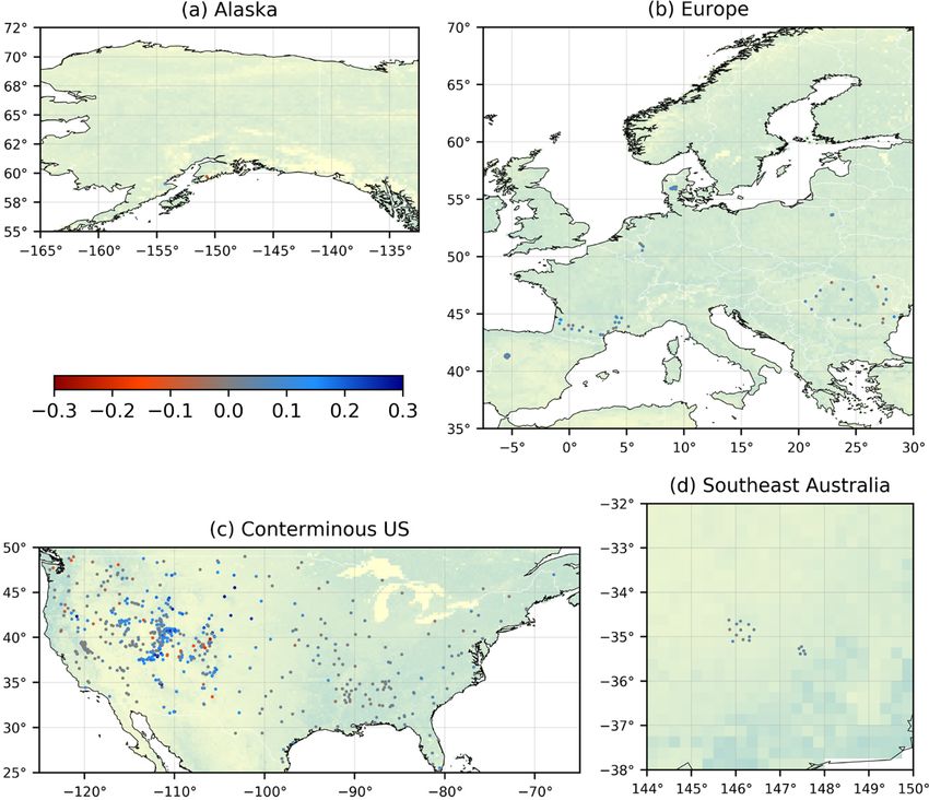
Figure 5. Three-hourly Pearson correlations (R) obtained by MeMo minus those obtained by ESA-CCI. Blue indicates that MeMo performs
better, whereas red indicates that ESA-CCI performs better. A map of long-term mean LAI (Baret et al., 2016) is plotted in the background.
This order matches the overall performance ranking of pre- SMAPL4) are not necessarily more accurate than those from
cipitation datasets in a comprehensive evaluation over the relatively simple, calibrated models (HBV). This is in line
conterminous USA carried out by Beck et al. (2019a). Fur- with several previous multi-model evaluations focusing on
thermore, the performance of HBV-ERA5 did not depend soil moisture (e.g., Guswa et al., 2002; Cammalleri et al.,
on the terrain slope, while HBV-IMERG performed worse 2015; Orth et al., 2015), the surface energy balance (e.g.,
in steep terrain (Fig. 3d), which is also consistent with the Best et al., 2015), evaporation (e.g., McCabe et al., 2016),
evaluation of Beck et al. (2019a). HBV-IMERG performed runoff (e.g., Beck et al., 2017a), and river discharge (e.g.,
worse for low-frequency than for high-frequency fluctuations Gharari et al., 2020).
(Fig. 4), which likely reflects the presence of seasonal biases
in IMERG (Beck et al., 2017c; Wang and Yong, 2020). Over- 3.6 How do the models with satellite data assimilation
all, these results confirm that precipitation is by far the most perform?
important determinant of soil moisture simulation perfor-
mance (Gottschalck et al., 2005; Liu et al., 2011; Beck et al., The performance ranking of the models with satellite data
2017c; Dong et al., 2019; Chen and Yuan, 2020). The supe- assimilation in terms of median R (from best to worst)
rior performance of MSWEP is primarily attributable to the was HBV-MSWEP+SMAPL3E, HBV-ERA5+SMAPL3E,
inclusion of daily gauge observations (Beck et al., 2019b). GLEAM, SMAPL4, HBV-IMERG+SMAPL3E, and ERA5
Among the three soil moisture products derived from (Fig. 3a; Table 1). The assimilation of SMAPL3E retrievals
ERA5 precipitation (ERA5, ERA5-Land, and HBV- resulted in a substantial improvement in median R of +0.06
ERA5) and among the three products forced with for HBV-IMERG, a minor improvement of +0.01 for HBV-
daily gauge-corrected precipitation (GLEAM, HBV- ERA5, and no change for HBV-MSWEP (Fig. 3a). Improve-
MSWEP+SMAPL3E, and SMAPL4; Table 1), the ones ments in R were obtained for 90 %, 65 %, and 56 % of
based on HBV performed better overall in terms of all three the sites for HBV-IMERG, HBV-ERA5, and HBV-MSWEP,
metrics (R, Rlo , and Rhi ; Figs. 3a and 4). This demonstrates respectively. For HBV-IMERG, the greatest improvements
that soil moisture estimates from complex data-intensive were found over the central Rocky Mountains (Fig. 6), where
models (H-TESSEL underlying ERA5 and ERA5-Land, IMERG performs relatively poorly (Beck et al., 2019a).
GLEAM, and the NASA Catchment model underlying Overall, these results suggest that data assimilation provides
greater benefits when the precipitation forcing is more uncer-
https://doi.org/10.5194/hess-25-17-2021 Hydrol. Earth Syst. Sci., 25, 17–40, 202128 H. E. Beck et al.: Evaluation of 18 satellite- and model-based soil moisture products
tain. Since rain gauge observations are not available over the els with randomly generated (uncalibrated) parameters ob-
large majority of the globe (Kidd et al., 2017), we expect tained mean median R values of 0.59, 0.53, and 0.62, re-
data assimilation to provide significant added value at the spectively (standard deviations 0.17, 0.16, and 0.16, respec-
global scale, as also concluded by Bolten et al. (2010), Dong tively; data not shown). The calibration thus resulted in mean
et al. (2019), and Tian et al. (2019). The lack of improvement increases in median R of +0.15, +0.12, and +0.16, respec-
for HBV-ERA5+SMAPL3E and HBV-MSWEP+SMAPL3E tively, for the three models, which represent substantial im-
suggests that the gain parameter G (Eq. 3), which quantifies provements in performance. These results are in line with
the relative quality of the satellite and model soil moisture previous studies calibrating different models using soil mois-
estimates, can be refined further. ture from in situ sensors (e.g., Koren et al., 2008; Shellito
The ERA5 reanalysis, which assimilates ASCAT soil et al., 2016b; Thorstensen et al., 2016; Reichle et al., 2019b)
moisture (Hersbach et al., 2020), obtained a lower overall or remote sensing (e.g., Zhang et al., 2011; Wanders et al.,
performance (median R = 0.68) than the open-loop mod- 2014; López López et al., 2016; Koster et al., 2018).
els ERA5-Land (median R = 0.72) and HBV-ERA5 (median The mean improvements in median R obtained for HBV-
R = 0.74), which were both forced with ERA5 precipita- ERA5, HBV-IMERG, and HBV-MSWEP after calibration
tion (Fig. 3a). This suggests that assimilating satellite soil (+0.15, +0.12, and +0.16, respectively) were significantly
moisture estimates (ERA5) was less beneficial than either greater than the improvements obtained for the same three
increasing the model resolution (ERA5-Land) or improv- models after satellite data assimilation (+0.01, +0.06, and
ing the soil moisture simulation efficiency (HBV). In line 0.00, respectively; Fig. 3a; Sect. 3.6), which suggests that
with these results, Muñoz Sabater et al. (2019) found that model calibration results in more benefit overall than data as-
the joint assimilation of ASCAT soil moisture retrievals and similation. Additionally, model calibration benefits regions
SMOS brightness temperatures into an experimental version with both sparse and dense rain gauge networks, whereas
of the Integrated Forecast System (IFS) model underlying data assimilation mainly benefits regions with sparse rain
ERA5 did not improve the soil moisture simulations. They gauge networks (Sect. 3.6). Conversely, only data assimila-
attributed this to the adverse impact of simultaneously as- tion is capable of ameliorating potential deficiencies in the
similated screen-level temperature and relative humidity ob- meteorological forcing data (e.g., undetected precipitation).
servations on the soil moisture estimates. Our calibration approach was relatively simple and yielded
In line with our results for HBV-MSWEP+SMAPL3E, only a single spatially uniform parameter set (Sect. 2.3).
Kumar et al. (2014) did not obtain improved soil moisture Previous studies focusing on runoff have demonstrated the
estimates after the assimilation of ESA-CCI and AMSR-E value of more sophisticated calibration approaches yielding
retrievals into Noah forced with highly accurate NLDAS2 ensembles of parameters that vary according to climate and
meteorological data for the conterminous USA. Conversely, landscape characteristics (Samaniego et al., 2010; Beck et al.,
several other studies obtained substantial performance im- 2016, 2020). Whether these approaches have value for soil
provements after data assimilation despite the use of high- moisture estimation as well warrants further investigation. It
quality precipitation forcings (Liu et al., 2011; Koster et al., should be noted, however, that many current models have
2018; Tian et al., 2019). We suspect that this discrepancy rigid structures, insufficient free parameters, and/or a high
might reflect the lower performance of their open-loop mod- computational cost which makes them less amenable to cali-
els compared to ours. Using different (but overlapping) in bration (Mendoza et al., 2015). Moreover, the validity of cal-
situ datasets, Koster et al. (2018) and Tian et al. (2019) ob- ibrated parameters may be compromised when the model is
tained mean daily open-loop R values of 0.64 and 0.59, re- subjected to climate conditions it has never experienced be-
spectively, while we obtained a mean daily open-loop R of fore (Knutti, 2008). Care should also be taken that calibra-
0.75 (slightly lower than the 3-hourly median value shown in tion of one aspect of the model does not degrade another as-
Fig. 3a). Overall, it appears that the benefits of data assimila- pect and that we get “the right answers for the right reasons”
tion are greater for models that exhibit structural or parame- (Kirchner, 2006).
terization deficiencies.
3.8 How do the major product categories compare?
3.7 What is the impact of model calibration?
The median R ± interquartile range across all sites and
Among the models evaluated in this study, only HBV and products in each category was 0.53 ± 0.32 for the satellite
the NASA Catchment model underlying SMAPL4 have been soil moisture products without SWI filter, 0.66 ± 0.30 for
calibrated against in situ soil moisture measurements, al- the satellite soil moisture products with SWI filter including
though only a single parameter out of more than 100 was MeMo, 0.69±0.25 for the open-loop models, and 0.72±0.22
calibrated for the Catchment model (Reichle et al., 2019b). for the models with satellite data assimilation (Fig. 3a; Ta-
HBV-ERA5, HBV-IMERG, and HBV-MSWEP with cali- ble 1). The satellite products thus provided the least reliable
brated parameters obtained median R values of 0.74, 0.65, soil moisture estimates and exhibited the largest regional per-
and 0.78, respectively (Fig. 3a), whereas the same three mod- formance differences on average, whereas the models with
Hydrol. Earth Syst. Sci., 25, 17–40, 2021 https://doi.org/10.5194/hess-25-17-2021H. E. Beck et al.: Evaluation of 18 satellite- and model-based soil moisture products 29
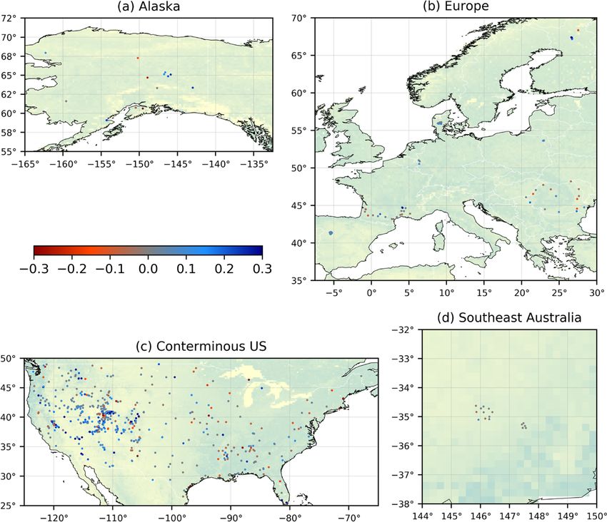
Figure 6. Three-hourly Pearson correlations (R) obtained by HBV-IMERG+SMAPL3E minus those obtained by HBV-IMERG. Blue indi-
cates improved performance after data assimilation, whereas red indicates degraded performance after data assimilation. The sites in Alaska
and Finland are not shown as IMERG does not cover high latitudes. A map of long-term mean LAI (Baret et al., 2016) is plotted in the
background.
satellite data assimilation provided the most reliable soil satellite data assimilation is due to the fact that individual er-
moisture estimates and exhibited the smallest regional per- rors in satellite retrievals and model estimates are canceled
formance differences on average. Our performance ranking out, to a certain degree, when they are combined, confirming
of the major product categories is consistent with previous the effectiveness of the data assimilation procedures (Morad-
studies for the conterminous USA (Liu et al., 2011; Kumar khani, 2008; Liu et al., 2012; Reichle et al., 2017).
et al., 2014; Fang et al., 2016; Dong et al., 2020), Europe
(Naz et al., 2019), and the globe (Albergel et al., 2012; Tian 3.9 To what extent are our results generalizable to
et al., 2019; Dong et al., 2019). It should be kept in mind, other regions?
however, that these studies, including the present one, used in
situ soil moisture measurements from regions with dense rain The large majority (98 %) of the in situ soil moisture mea-
gauge networks and hence likely overestimate model perfor- surements used as reference in the current study was from
mance (Dong et al., 2019). dense monitoring networks in the USA and Europe (Fig. 2);
The large spread in performance across the satellite prod- therefore, our results will be most applicable to these regions.
ucts reflects the large number of factors that affect soil mois- We speculate that our results for the models (with and with-
ture retrieval, including, among others, vegetation cover, out data assimilation; Figs. 3, 4, and 6) apply to other re-
surface roughness, soil composition, diurnal variations in gions with dense rain gauge networks and broadly similar
land surface conditions, and RFI (Zhang and Zhou, 2016; climates (e.g., parts of China and Australia and other parts
Karthikeyan et al., 2017b). The spread in performance across of Europe; Kidd et al., 2017). The calibrated models (HBV
the open-loop models is lower as it depends primarily on the and the NASA Catchment model underlying SMAPL4) may,
precipitation data quality, which, in turn, depends mostly on however, perform slightly worse in regions with climatic
a combination of gauge network density and prevailing pre- and physiographic conditions dissimilar to the in situ sen-
cipitation type (convective versus frontal; Gottschalck et al., sors used for calibration (but likely still better than the un-
2005; Liu et al., 2011; Beck et al., 2017c; Dong et al., 2019). calibrated models). In sparsely gauged areas the four model
The smaller spread in performance across the models with products based on precipitation forcings that incorporate
daily gauge observations (GLEAM, HBV-MSWEP, HBV-
https://doi.org/10.5194/hess-25-17-2021 Hydrol. Earth Syst. Sci., 25, 17–40, 202130 H. E. Beck et al.: Evaluation of 18 satellite- and model-based soil moisture products
MSWEP+SMAPL3E, and SMAPL4; Table 1) will inevitably 2. Application of the SWI smoothing filter resulted in im-
exhibit lower performance (but not necessarily lower than proved performance for all satellite products. Previous
the other model products). In convection-dominated regions near-surface soil moisture product assessments gener-
models driven by precipitation from satellite datasets such as ally did not apply smoothing filters and therefore may
IMERG may well outperform those driven by precipitation have underestimated the true skill of the products.
from reanalyses such as ERA5 (Massari et al., 2017; Beck
et al., 2017c, 2019b). Conversely, in mountainous and snow- 3. SMAPL3ESWI performed best overall among the
dominated regions models driven by precipitation from re- four single-sensor satellite products with SWI filter.
analyses are likely to outperform those driven by precipita- ASCATSWI performed markedly better in terms of high-
tion from satellites (Ebert et al., 2007; Beck et al., 2019b, a). frequency than low-frequency fluctuations. All satellite
Our results for the satellite soil moisture products may products tended to perform worse in cold climates.
be less generalizable, given the large spread in performance 4. The multi-sensor merged satellite product MeMo per-
across different regions and products revealed in the current formed best among the satellite products, highlighting
study (Figs. 3 and 4) and in previous quasi-global studies the value of multi-sensor merging techniques. MeMo
using triple collocation (Al-Yaari et al., 2014; Chen et al., also outperformed the multi-sensor merged satellite
2018; Miyaoka et al., 2017). Outside developed regions we product ESA-CCISWI , likely due to the inclusion of
expect the lower prevalence of RFI to lead to more reliable SMAPL3ESWI .
retrievals for those satellite products susceptible to it (Njoku
et al., 2005; Oliva et al., 2012; Aksoy and Johnson, 2013; 5. The performance of the open-loop models depended
Ticconi et al., 2017). At low latitudes the lower satellite re- primarily on the precipitation data quality. The superior
visit frequency will inevitably increase the sampling uncer- performance of HBV-MSWEP is due to the calibration
tainty and reduce the overall value of satellite products rela- of HBV and the daily gauge corrections of MSWEP.
tive to models. In tropical forest regions passive products of- Soil moisture simulation performance did not improve
ten do not provide soil moisture retrievals, and when they do, with model complexity.
the retrievals are typically less reliable than those from active
products due to the dense vegetation cover (Al-Yaari et al., 6. In the absence of model structural or parameterization
2014; Chen et al., 2018; Miyaoka et al., 2017; Kim et al., deficiencies, satellite data assimilation yields substan-
2018). Shedding more light on the strengths and weaknesses tial performance improvements mainly when the precip-
of soil moisture products in regions without dense measure- itation forcing is of relatively low quality. This suggests
ment networks – for example using independent soil mois- that data assimilation provides significant benefits at the
ture products (Chen et al., 2018; Dong et al., 2019) or by global scale.
expanding measurement networks (Kang et al., 2016; Singh 7. The calibration of HBV against in situ soil moisture
et al., 2019) – should be a key priority for future research measurements resulted in substantial performance im-
(Ochsner et al., 2013; Myeni et al., 2019). provements. The improvement due to model calibration
tends to exceed the improvement due to satellite data
4 Conclusions assimilation and is not limited to regions of low-quality
precipitation data.
To shed light on the advantages and disadvantages of differ-
8. The satellite products provided the least reliable soil
ent soil moisture products and on the merit of various tech-
moisture estimates and exhibited the largest regional
nological and methodological innovations, we evaluated 18
performance differences on average, whereas the mod-
state-of-the-art (sub-)daily (quasi-)global near-surface soil
els with satellite data assimilation provided the most re-
moisture products using in situ measurements from 826 sen-
liable soil moisture estimates and exhibited the smallest
sors located primarily in the USA and Europe. Our main find-
regional performance differences on average.
ings related to the nine questions posed in the introduction
can be summarized as follows: 9. We speculate that our results for the models (with and
without data assimilation) apply to other regions with
1. Local night retrievals from descending overpasses were
dense rain gauge networks and broadly similar climates.
more reliable overall for AMSR2, whereas local morn-
Our results for the satellite products may be less gener-
ing retrievals from descending overpasses were more re-
alizable due to the large number of factors that affect
liable overall for ASCAT. The ascending and descend-
retrievals.
ing retrievals of SMAPL3E and SMOS performed sim-
ilarly.
Hydrol. Earth Syst. Sci., 25, 17–40, 2021 https://doi.org/10.5194/hess-25-17-2021You can also read