From model to radar variables: a new forward polarimetric radar operator for COSMO - Atmos. Meas. Tech
←
→
Page content transcription
If your browser does not render page correctly, please read the page content below
Atmos. Meas. Tech., 11, 3883–3916, 2018
https://doi.org/10.5194/amt-11-3883-2018
© Author(s) 2018. This work is distributed under
the Creative Commons Attribution 4.0 License.

From model to radar variables: a new forward polarimetric
radar operator for COSMO
Daniel Wolfensberger and Alexis Berne
LTE, Ecole polytechnique fédérale de Lausanne (EPFL), Lausanne, Switzerland

Correspondence: Alexis Berne (alexis.berne@epfl.ch)

Received: 27 November 2017 – Discussion started: 21 December 2017
Revised: 12 May 2018 – Accepted: 7 June 2018 – Published: 4 July 2018

Abstract. In this work, a new forward polarimetric radar op-          tool to evaluate and test the microphysical parameterizations
erator for the COSMO numerical weather prediction (NWP)               of the model.
model is proposed. This operator is able to simulate mea-
surements of radar reflectivity at horizontal polarization, dif-
ferential reflectivity as well as specific differential phase shift
and Doppler variables for ground based or spaceborne radar            1   Introduction
scans from atmospheric conditions simulated by COSMO.
The operator includes a new Doppler scheme, which al-                 Weather radars deliver areal measurements of precipitation
lows estimation of the full Doppler spectrum, as well a               at a high temporal and spatial resolution. Most recent op-
melting scheme which allows representing the very spe-                erational weather radar systems have dual-polarization and
cific polarimetric signature of melting hydrometeors. In ad-          Doppler capabilities (called polarimetric below), which pro-
dition, the operator is adapted to both the operational one-          vide not only information about the intensity of precipita-
moment microphysical scheme of COSMO and its more ad-                 tion, but also about the type of precipitation (e.g., phase,
vanced two-moment scheme. The parameters of the relation-             homogeneity and shape of hydrometeors). Additionally, the
ships between the microphysical and scattering properties of          Doppler capability of weather radars allows monitoring the
the various hydrometeors are derived either from the liter-           radial velocity of hydrometeors. In view of their capacities,
ature or, in the case of graupel and aggregates, from ob-             weather radars offer great opportunities for validation of and
servations collected in Switzerland. The operator is evalu-           assimilation in numerical weather prediction (NWP) models.
ated by comparing the simulated fields of radar observables           This is unfortunately far from being a trivial task since radar
with observations from the Swiss operational radar network,           observables that are derived from the backscattered power
from a high resolution X-band research radar and from the             and phase from precipitation cannot be simply put into re-
dual-frequency precipitation radar of the Global Precipitation        lation with the state of the atmosphere as simulated by the
Measurement satellite (GPM-DPR). This evaluation shows                model. There is thus the need for a conversion tool, able to
that the operator is able to simulate an accurate Doppler spec-       simulate synthetic radar observations from simulated model
trum and accurate radial velocities as well as realistic dis-         variables: a so-called forward radar operator.
tributions of polarimetric variables in the liquid phase. In             Over the past few years, several forward radar operators
the solid phase, the simulated reflectivities agree relatively        have been developed. One of the first efforts was made by
well with radar observations, but the simulated differential          Pfeifer et al. (2008) who designed a polarimetric operator
reflectivity and specific differential phase shift upon propaga-      for the COSMO model, able to simulate horizontal reflec-
tion tend to be underestimated. This radar operator makes it          tivity ZH , differential reflectivity ZDR , and linear depolar-
possible to compare directly radar observations from various          ization ratio (LDR) observations. The operator relies on the
sources with COSMO simulations and as such is a valuable              T-matrix method (Mishchenko et al., 1996) to estimate scat-
                                                                      tering properties of individual hydrometeors. Assumptions
                                                                      about shape, density, and canting angles, which cannot be ob-

Published by Copernicus Publications on behalf of the European Geosciences Union.
3884               D. Wolfensberger and A. Berne: A forward polarimetric radar operator for the COSMO NWP model

tained from the NWP model were obtained from a sensitivity         proximation that can be specified. Note that the operator is
study. A limitation of this operator is that it does not per-      currently not able to simulate polarimetric variables.
form any integration over the antenna power density pattern           Most available radar operators are primarily designed to
and thus neglects the beam broadening effect which can be          simulate operational PPI (plane position indicator) scans
quite significant at longer distances from the radar (Ryzhkov,     from operational weather radars at S, C, or X bands. How-
2007).                                                             ever, in research, other types of radar data are available which
   Cheong et al. (2008) developed a three-dimensional              can also be relevant in the evaluation of a NWP model, es-
stochastic radar simulator able to simulate raw time series of     pecially for the simulated vertical structure of precipitation.
weather radar data. Doppler characteristics are retrieved by       Some examples of radar data used for research include satel-
moving discrete scatterers with the three-dimensional model        lite swaths at higher frequencies, such as measurements of
wind field, which allows producing sample-to-sample time           the GPM-DPR satellite at Ku and Ka band (Iguchi et al.,
series data, instead of theoretical moments as with conven-        2003) as well as power weighted distributions of scatterer
tional radar simulators. Thanks to this, the radar simulator is    radial velocities (Doppler spectra), commonly recorded by
able to generate the full Doppler spectrum; however, this is       many research radars.
at the expense of a high computation cost and without taking          The purpose of this work is to design a state of the art
attenuation into account.                                          forward polarimetric radar operator for the COSMO NWP
   Jung et al. (2008) developed a polarimetric radar operator      model taking into account the physical aspects of beam prop-
able to simulate ZH , ZDR as well as the specific differential     agation and scattering as accurately as possible, while en-
phase on propagation Kdp and adapted it for two different          suring a reasonable computation time on a standard desktop
microphysical schemes: one single-moment scheme and one            computer. The radar operator also needs to be versatile and
two-moment scheme. The authors also proposed a method to           able to simulate a variety of radar variables at many frequen-
simulate the effect of the melting layer with a weather model      cies and for different microphysical schemes, in order to be
that does not explicitly simulate wet hydrometeors. They           used in the future as a model evaluation tool with operational
used this operator to simulate realistic polarimetric radar sig-   and research weather radar data. As such, this radar operator
natures of a supercell storm from simulations obtained with        includes a number of innovative features: (1) the ability to
the Advanced Regional Prediction System (ARPS; Xue et al.,         simulate the full Doppler spectrum at a very low computa-
2000). However, the validation of the operator was limited to      tional cost, (2) the ability to simulate observations from both
idealized cases at S-band only.                                    ground and spaceborne radars, (3) a probabilistic parameteri-
   Ryzhkov et al. (2011) developed an advanced forward             zation of the properties of solid hydrometeors derived from a
radar operator for a research cloud model with spectral mi-        large dataset of observations in Switzerland, (4) the inclusion
crophysics able to simulate ZH , ZDR , LDR, and Kdp . Scat-        of cloud hydrometeors (which contribution becomes impor-
tering amplitudes of smaller particles are estimated with the      tant at higher frequencies). Besides, the radar operator has
Rayleigh approximation whereas the T-matrix method is              been thoroughly evaluated using a large selection of radar
used for larger hydrometeors. However, note that this cloud        data at different frequencies and corresponding to various
model is computationally expensive and is not used for oper-       synoptic conditions.
ational weather prediction.                                           The article is structured as follows: in Sect. 2, a description
   Augros et al. (2016) elaborated a polarimetric forward          of the COSMO NWP model as well as the radar data used for
radar operator for the French non-hydrostatic mesoscale re-        the evaluation of the operator is given. In Sect. 3, the differ-
search NWP model Meso-NH (Lafore et al., 1998) based on            ent steps of the polarimetric radar operator are extensively
the forward conventional radar operator of Caumont et al.          described and its assumptions are discussed in details. Sec-
(2006) which simulates all operational polarimetric radar ob-      tion 4 focuses on the qualitative and quantitative evaluation
servables: ZH , ZDR , the differential phase shift upon propa-     of the simulated radar observables using real radar obser-
gation φDP , the co-polar correlation coefficient ρhv and Kdp .    vations from both operational and research ground weather
The operator uses the T-matrix method for rain, snow, and          radars, as well as GPM satellite data. Finally, Sect. 5 sum-
graupel particles and Mie scattering for pristine ice particles.   marizes the main results and opens perspectives for possible
Beam-broadening is taken into account by approximating the         applications of the operator.
integration over the antenna normalized power density pat-
tern with a Gauss–Hermite quadrature scheme.
   Finally, Zeng et al. (2016) developed a forward radar oper-     2     Description of the data
ator for the COSMO model. The operator is designed for op-
erational purposes (assimilation and validation) with an em-       2.1    COSMO model
phasis on performance and modularity. It simulates Doppler
velocity with fall speed and reflectivity weighting as well as     The COSMO Model is a mesoscale limited area model ini-
attenuated horizontal reflectivity, with different levels of ap-   tially developed as the Lokal-Modell (LM) at the Deutscher
                                                                   Wetterdienst (DWD). It is now operated and developed by

Atmos. Meas. Tech., 11, 3883–3916, 2018                                               www.atmos-meas-tech.net/11/3883/2018/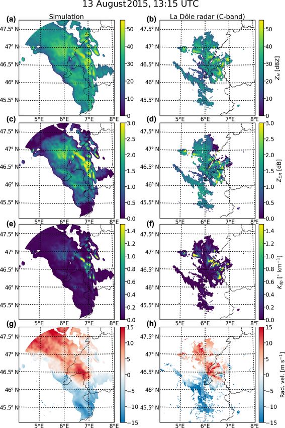
D. Wolfensberger and A. Berne: A forward polarimetric radar operator for the COSMO NWP model                               3885

several weather services in Europe (Switzerland, Italy, Ger-      of snow, to be temperature dependent. µ is equal to zero (ex-
many, Poland, Romania, and Russia). Besides its opera-            ponential PSDs) for all hydrometeors, except for rain where
tional applications, it is also used for scientific purposes in   it is set to 0.5 by default and ν is always equal to one.
weather dynamics, microphysics and prediction and for re-             In the two-moment scheme, both 3 and N0 are prognostic
gional climate simulations. The COSMO Model is a non-             parameters, and can be obtained from the prognostic moment
hydrostatic model based on the fully compressible primitive       of order zero (number concentration) and from the mass con-
equations integrated using a split-explicit third-order Runge–    centration. µ and ν are defined a priori.
Kutta scheme (Wicker and Skamarock, 2002). The spatial                Table 1 gives the values of the PSD parameters µ, N0 , and
discretization is based on a fifth-order upstream advection       ν as well as the mass–diameter power-law parameters a and
scheme on an Arakawa C-grid with Lorenz vertical stag-            b and the terminal velocity–diameter power-law parameters
gering. Height-based Gal-Chen coordinates are used in the         α and β for all hydrometeor types and the two microphysical
vertical (Gal-Chen and Somerville, 1975). The model uses          schemes.
a rotated coordinate system where the pole is displaced to            Non-precipitating quantities (cloud droplets and cloud ice)
ensure approximatively horizontal resolution over the model       do not have a spectral representation in the one-moment
domain. Sub-grid scale processes are taken into account with      scheme of COSMO, but are instead treated as bulk, with the
parameterizations.                                                total number of particles being a function of the air tempera-
   In COSMO, grid-scale clouds and precipitation are pa-          ture.
rameterized operationally with a one-moment scheme sim-               In the operational setup, for the parameterization of at-
ilar to Rutledge and Hobbs (1983) and Lin et al. (1983), with     mospheric turbulence, the COSMO model uses a prognostic
five hydrometeor categories: rain, snow, graupel, ice crys-       turbulent kinetic energy (TKE) closure at level 2.5 similar to
tals, and cloud droplets. Snow is assumed to be in the form       (Mellor and Yamada, 1982). The main difference is the use of
of rimed aggregates of ice-crystals that have become large        variables that are conserved under moist adiabatic processes:
enough to have an appreciable fall velocity. Cloud ice is as-     total cloud water and liquid water potential temperature. Ad-
sumed to be in the form of small hexagonal plates. In the         ditionally, a so-called “circulation term” is included which
version of COSMO that is being used (5.04), ice crystals          describes the transfer of nonturbulent subgrid kinetic energy
have a bulk non-diameter dependent terminal velocity, that        from larger-scale circulation toward TKE. The reader is re-
depends on their mass concentration. The particle size distri-    ferred to Baldauf et al. (2011) and the model documentation
butions (PSD) are assumed to be exponential for all hydrom-       (Doms et al., 2011) for a more in-depth description of the
eteors, except for rain where a gamma PSD is assumed. A           various COSMO sub-grid parameterizations.
more advanced two-moment scheme with a sixth hydrome-
teor category, hail, was developed for COSMO by Seifert and       2.2   Radar data
Beheng (2006) and extended by Blahak (2008) and Noppel
et al. (2010). As this scheme significantly increases the over-   For the evaluation of polarimetric variables, the final prod-
all computation time it is currently not used operationally.      uct from the Swiss operational radar network was used. The
   In COSMO, with the exception of ice crystals and rain in       Swiss network consists of five polarimetric C-band radars,
the two-moment scheme, mass–diameter relations as well as         performing PPI scans at 20 different elevation angles (Ger-
velocity–diameter relations are assumed to be power-laws.         mann et al., 2006). The final quality-checked measurements
For rain in the two-moment scheme, a slightly more refined        are corrected for ground clutter, calibrated and aggregated
formula by Rogers et al. (1993) is used. For ice crystals,        at a resolution of 500 m. In this work, ZH was used as pro-
the two-moment scheme, in contrast with the one-moment            vided, ZDR was corrected with a daily radar-dependent cal-
scheme uses a spectral (diameter-dependent) representation        ibration constant provided by MeteoSwiss, and Kdp was es-
of ice crystal terminal velocities. For both microphysical        timated from 9DP using the Kalman filter ensemble method
schemes, all PSDs can be expressed as particular cases of         of Schneebeli et al. (2013). Note that two of the operational
generalized gamma PSDs.                                           radars were installed only recently (2014 and 2016) and were
                                                                  thus not used in this study (see Fig. 1).
                                                                     For the evaluation of simulated Doppler variables (mean
N(D) = N0 D µ exp −3 · D ν        m−3 mm−1 ,

                                                           (1)
                                                                  radial velocity and Doppler spectrum at vertical incidence),
where N0 is the intercept parameter in units of                   observations from a mobile X-band radar (MXPol) deployed
mm−1−µ m−3 , µ is the dimensionless shape parameter,              in Payerne in Western Switzerland in Spring 2014 were used.
3 is the slope parameter in units of mm−ν and ν is the            The radar was deployed in the context of the PARADISO
dimensionless family parameter.                                   measurement campaign (Figueras i Ventura et al., 2015). The
   In the one-moment scheme, which is used operationally,         PARADISO dataset provides a great opportunity to evalu-
the only free parameter of the PSDs is 3 which can be ob-         ate the simulated radial velocities, as Payerne is the location
tained from the prognostic mass concentrations. N0 is either      from which the radiosoundings, which are assimilated every
assumed to be constant during the simulation, or in the case      3 h in the model, are launched.

www.atmos-meas-tech.net/11/3883/2018/                                              Atmos. Meas. Tech., 11, 3883–3916, 2018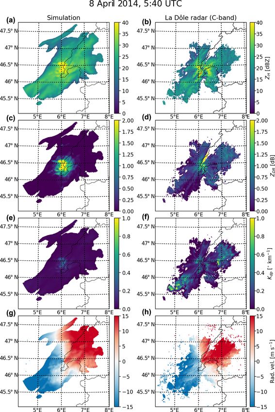
3886 D. Wolfensberger and A. Berne: A forward polarimetric radar operator for the COSMO NWP model
Table 1. Parameters of the hydrometeor PSDs and power-laws for the two microphysical schemes (separated by a slash sign). ∅ indicates
that the hydrometeor is not simulated in this scheme, a dash indicates that this parameter is not used in this parameterization, and “free”
indicates a prognostic parameter. As in Eq. (1), N0 is expressed in units of mm−1−µ m−3 . Note that the value of µ for rain can be specified
in the COSMO user set-up, 0.5 being the default value. The parameters a and b correspond to the power-law: m(D) = aD b , with m is in kg
and D in mm. The parameters α and β correspond to the power-law: vt (D) = αD β , with vt being the terminal fall velocity in m s−1 , and D
is the diameter in mm.
Rain Snow Graupel Hail Ice crystals
N0 1253/free 1 /free 4000/free ∅/free −/free
µ 0.5/2 0/1.2 0/5.37 ∅/5 −/2.311
ν 1/1 1/1.1 1/1.06 ∅/1 −/1.104
a 5.23 ×10⁻⁷ / 3.80 ×10⁻⁸ / 8.50 ×10⁻⁸ / ∅/ 1.3 ×10⁻⁷ /
5.24 ×10⁻⁷ 3.80 ×10⁻⁸ 8.50 ×10⁻⁸ 3.39 ×10⁻⁷ 1.17 ×10⁻⁷
b 3.00/3.00 2.00/2.00 3.10/3.10 ∅/3.00 3.00/3.31
α 4.11/− 0.871/0.871 0.945/1.258 ∅/3.362 −/0.966
β 0.50/− 0.25/0.20 0.89/0.85 ∅/0.50 −/1.20
1 for snow, a relation of N with the temperature is used (Field et al., 2005).
0
An overview of the specifications of all radars used in this Altitude [m]
4500
study is given in Table 2. The location of the Swiss oper- 4100
3700
3300
ational radars used in the evaluation of the radar operator 2900
2500
(Sect. 4.3) and their maximum considered range (100 km) are 2100
1700
shown in Fig. 1. 1300
900
500
Besides ground radar data, measurements from the dual-
frequency precipitation radar (DPR, Furukawa et al., 2016),
on-board the core satellite of the Global Precipitation Mea-
surement mission (GPM, Iguchi et al., 2003) were used
to validate the simulation of spaceborne radar swaths. The
GPM-DPR radar operates at both Ku (13.6 GHz) and Ka
(35.6 GHz) bands. At Ku-band, the satellite swath covers ap-
proximately 245 km in width, with a horizontal resolution ap-
proximatively 5 km and a 250 m vertical (radial) resolution.
At Ka-band, the satellite swath is more narrow, covering only
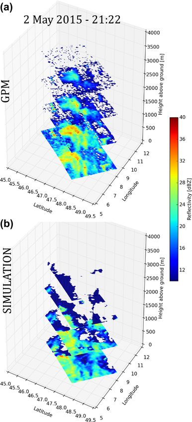
125 km in width. Figure 1. Location of the Swiss operational radars. The three radars
used in the context of this study are surrounded by black circles
2.3 Parsivel data which indicate the maximum range of radar data (100 km) used for
the evaluation of the radar operator (Sect. 4.3). Note that as they
In order to compare the COSMO drop size distribution were installed only quite recently, no data from the Weissfluhgipfel
parameterizations with real observations, data from three and Plaine Morte radars were used in this study.
Parsivel-1 optical disdrometers were used. These instruments
were deployed at a short distance from each other, near
the Payerne MeteoSwiss station. Like the X-band radar pre-
sented above, these instruments were deployed in the context 2.4 Precipitation events
of the PARADISO measurement campaign. The measured
drop size distributions were corrected with measurements
A list and short description of all five events used for the
from a 2-dimensional video disdrometer (2DVD) using the
evaluation of the radar operator with data from the opera-
method of Raupach and Berne (2015). For more details re-
tional C-band radars (Sect. 4.3) and all six events from the
garding these instruments, see Raupach and Berne (2015).
PARADISO campaign used for the evaluation of the radar
All disdrometers were located within the same COSMO grid
operator with data from MXPol (Sect. 4.2) and from Parsivel
cell, so the measured DSDs were simply averaged before
data (Sect. 4.4) is given in Table 3.
comparing them with the COSMO parameterizations.
For the comparison of simulated GPM swaths with real
observations, the 100 overpasses with the largest precipita-
tion fluxes recorded between March 2014 and the end of
2016 were selected. Overall, this selection is a balanced
Atmos. Meas. Tech., 11, 3883–3916, 2018 www.atmos-meas-tech.net/11/3883/2018/
D. Wolfensberger and A. Berne: A forward polarimetric radar operator for the COSMO NWP model                                        3887

Table 2. Specifications of the ground radars used in the evaluation of the radar operator.

                                                 MXPol                    Swiss radar network
                   Location                      Payerne: 46.813◦ N,      Albis: 47.284◦ N, 8.512◦ E, 891 m a.s.l.
                                                 6.943◦ E, 495 m a.s.l.   La Dôle: 46.425◦ N, 6.099◦ E, 1680 m a.s.l.
                                                                          Monte Lema: 46.040◦ N, 8.833◦ E, 1604 m a.s.l.
                   Frequency f                   9.41 GHz (X-band)        5.6 GHz (C-band)
                   Pulse width τ                 0.5 µs                   0.577 µs
                   PRF                           1666 Hz                  500 to 1500 Hz (depends on elevation)
                   FFT length                    128                      −
                   3 dB beamwidth                1.45◦                    1◦
                   Sensitivity (SNR = 10 dB)     11 dBZ at 10 km          0 dBZ at 10 km

mix between widespread low-intensity precipitation and lo-
cal strong convective storms.

3     Description of the polarimetric radar operator

The radar operator simulates observations of ZH , ZDR , Kdp ,
average Doppler (radial) velocity, and of the full Doppler
spectrum based on COSMO simulations and user-specified
radar characteristics, such as its position, its frequency, the
3 dB antenna beamwidth 13 dB , the pulse duration τ , and the
pulse repetition frequency (PRF). Figure 2 summarizes the
main steps of this procedure, which will be more extensively
detailed in the further section.

3.1    Propagation of the radar beam

Microwaves in the atmosphere propagate along curved lines
at speeds v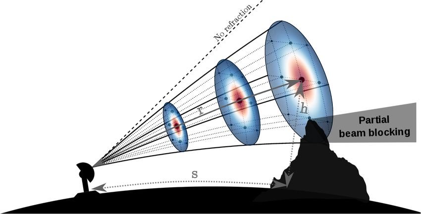
3888                D. Wolfensberger and A. Berne: A forward polarimetric radar operator for the COSMO NWP model

Table 3. List of all events used for the comparison of simulated radar observables with real ground radar observations. The last column
indicates the context of the comparison. A indicates the comparison with the operational C-band radars (Sect. 4.3), B indicates the comparison
with the X-band radar (Sect. 4.2), and the Parsivel data (Sect. 4.4) in Payerne and C indicates the evaluation of ice crystals with the X-band
radar in the Swiss Alps in Davos (Sect. 4.6).

                     Event                  Description                                                         Used
                                                                                                                for
                     1 February 2013        Heavy snowfall event with strong westerly geostrophic winds.        A
                     22 March 2014          Stationary front with widespread stratiform liquid precipitation    B
                                            over Switzerland.
                     8 April 2014           After the crossing of a cold front, presence of mostly liquid       A/B
                                            widespread stratiform precipitation over Switzerland.
                     1 May 2014             Occlusion over Switzerland with mild temperatures and               B
                                            widespread stratiform precipitation
                     7 May 2014             Wake of a cold front with scattered stratiform precipitation        B
                     11 May 2014            Wake of a cold front with strong scattered stratiform and occa-     B
                                            sionally convective precipitation
                     14 May 2014            Occlusion over Switzerland with mild temperatures and               B
                                            widespread stratiform precipitation
                     8 November 2014        The first two weeks of November 2014 were characterized by          A
                                            very heavy rainfall over the Southern Alps with strong Foehn
                                            winds, due to the presence of a very strong low pressure system
                                            over the Mediterranean (Xandra).
                     9 January 2015         Crossing of a warm front over Switzerland with widespread           C
                                            stratiform precipitation and snowfall over the Swiss Alps.
                     26 January 2015        Snowfall event over the Swiss Alps with very similar character-     C
                                            istics to the 9 January 2015 event
                     23 February 2015       Crossing of a cold front over Switzerland with some widespread      C
                                            and medium-intensity snowfall
                     13 August 2015         Strong summer convection triggered by the presence of very          A
                                            warm and wet subtropical air over Switzerland.
                     7 June 2016            Presence of warm and moist air over Western Europe with a           A
                                            succession of thunderstorms.

   The choice of the refraction model (Earth equivalent or               servables requires numerical integration over a particle size
atmospheric refraction) is left to the user of the radar opera-          distribution at every bin, which is costly. Secondly, comput-
tor, noting that the computation cost for the latter is slightly         ing radar observables after linear interpolation allows preser-
larger. The whole evaluation of the radar operator presented             vation of the mathematical relation between them. Indeed,
in Sect. 4 was performed with the more advanced model of                 radar variables are far from being independent. For example,
Zeng et al. (2014).                                                      in the liquid phase ZH is closely co-fluctuating with ZDR , in
                                                                         the form of a power-law that tends to stagnate at large re-
3.2    Interpolation of model variables                                  flectivities. Some tests were performed on random Gaussian
                                                                         fields of rain mass concentration. The results indicate that
Once the distance at the ground s and the height above                   when computing the radar observables first and then interpo-
ground h are obtained from the refraction model, it is easy              lating them, this theoretical relation becomes more and more
to retrieve the latitude, longitude, and height coordinates              linear when the interpolation resolution increases, which is
(ψ WGS , λWGS , h) of the corresponding radar gate, knowing              quite unrealistic. On the contrary, when computing the radar
the beam elevation θ0 and azimuth φ0 angles, as well as the              variables after interpolating the rain concentration field, the
position of the radar.                                                   theoretical relationship is always preserved, regardless of the
   Once the coordinates of all radar gates have been defined,            interpolation technique that is being used.
the model variables must be interpolated to the location of the             Technical details about the trilinear interpolation proce-
radar gates. This is done with trilinear interpolation (linear           dure are given in Appendix A.
interpolation in three dimensions). The advantage of interpo-
lating model variables before estimating radar observables,
instead of doing the opposite, is twofold. At first, it is much
more computationally efficient, because computing radar ob-

Atmos. Meas. Tech., 11, 3883–3916, 2018                                                      www.atmos-meas-tech.net/11/3883/2018/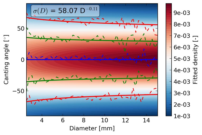
D. Wolfensberger and A. Berne: A forward polarimetric radar operator for the COSMO NWP model 3889
3.3 Retrieval of particle size distributions they do not have a spectral representation in the one-moment
scheme of COSMO. Instead, a realistic PSD is retrieved
In the one-moment scheme, for a given hydrometeor j , with the double-moment normalization method of Lee et al.
(j )
the COSMO specific mass concentration QM in kg m−3 is (2004). This formulation of the PSD requires to know two
proportional to a specific moment of the particle size dis- moments of the PSD as well as an appropriate normalized
tributions (PSD), since the COSMO parameterizations as- PSD function. Field et al. (2005) proposes best-fit relations
sumes simple power-laws for the mass–diameter relations: between the moments of ice crystals PSDs as well as fits of
(j )
m(j ) (D) = a (j ) D b . Because all COSMO PSDs belong to generating functions for different pair of moments. Precisely,
the class of generalized gamma PSDs, QM can be expressed assuming moments 2 (M2 ) and 3 (M3 ) of the size distribu-
as follows: tions are known, Field et al. (2005) suggest parameterizing
the PSD in the following way:
(j ) N (j ) (D)
M2
DZmax
N ice (D) = M42 · M−3 , (4)
z }| {
(j ) b(j ) (j ) µ(j ) (j ) ν (j ) 3 φ23 (x), with x = D
QM = a (j ) D · N0 D exp −3 D dD. (2) M3
(j )
Dmin with
φ23 (x) = 490.6 exp(−20.78x) + 17.46x 0.6357 exp(−3.290x). (5)
As in the COSMO microphysical parameterization (see
Doms et al., 2011), the PSDs are assumed to be only weakly Unfortunately, in the one-moment scheme of COSMO,
(j ) (j )
truncated and the integration bounds [Dmin , Dmax ] are re- only one single moment is known, which corresponds to
placed by [0, ∞), in order to get an analytical solution and M3 , since the value of the b parameter in the mass–diameter
avoid the cost of numerical root finding. Note that this trun- power-law for ice crystals is equal to 3 (see Table 1). Fortu-
cation hypothesis is done only for the retrieval of 3 and not nately, Field et al. (2005) also provide best-fit relations re-
when computing the radar observables (Sect. 3.6.2 and Ap- lating M2 to other moments of the PSD. According to these
pendix C). For the one-moment scheme, by integrating the relationships, M3 can be estimated from M2 with
Eq. (2), one gets the following expression for the free param-
eter 3(j ) . b(3, Tc )
M3 ≈ a(3, Tc )M2 , (6)
ν (j )
where a(3, Tc ) and b(3, Tc ) are polynomial functions of the
in-cloud temperature (in ◦ C) and the moment order (3 in this
(j ) b(j ) +µ(j ) +1
b(j ) +µ(j ) +1
N0 a (j ) 0 ν (j )
(j ) case).
31 mom = (j )
(3)
ν (j ) QM Taking advantage of these results, it is possible to retrieve
a PSD for ice crystals in the radar operator by (1) using the
For the two-moment scheme, the method is similar, ex- COSMO temperature to retrieve an estimate for a(3, Tc ) and
cept that both mass and number concentrations are needed to b(3, Tc ), (2) inverting Eq. (6) to get an estimate of M2 , and
retrieve 3 and N0 . The corresponding mathematical formu- (3) use Eqs. (4) and (5) to estimate the PSD of ice crystals.
lation is given in Appendix B.
Equation (3) allows retrieving the PSD parameters for all 3.4 Integration over the antenna pattern
hydrometeors1 in Table 1 at every radar gate using the model
(j ) Part of the transmitted power is directed away from the axis
variable QM , and, for the two-moment scheme, the prognos-
(j ) of the antenna main beam, which will increase the size of
tic number concentration QN (M0 ) as well. Knowing the the radar sampling volume with range, an effect known as
PSDs (N (j ) (D)) makes it possible to perform the integration beam-broadening. Depending on the antenna beamwidth this
of polarimetric variables over ensemble of hydrometeors as effect can be quite significant and needs to be accounted for
will be described in the next steps of the operator. by integrating the radar observables at every gate over the
In our radar operator, cloud droplets are neglected because antenna power density pattern. Equation (7) formulates the
the radar operator is designed for common precipitation radar antenna integration for an arbitrary radar observable y and a
frequencies (2.7 up to 35 GHz), for which the contribution normalized power density pattern of the antenna represented
of cloud droplets is very small (Fabry, 2015). However, at by f 2 , as in Doviak and Zrnić (2006).
higher frequencies and in weak precipitation, the contribu-
tion of ice crystals can be significant, especially for ZDR ,
as these crystals can be quite oblate (Battaglia et al., 2001). I y (ro , θo , φo ) =
Therefore, ice crystals are considered explicitly, even though ro +1
Z r /2 θo +π/2
Z φoZ+π
1 except for the ice crystals in the one-moment scheme, where y(r, θ, φ)
COSMO does not consider any spectral representation. ro −1r /2 θo −π/2 φo −π
www.atmos-meas-tech.net/11/3883/2018/ Atmos. Meas. Tech., 11, 3883–3916, 2018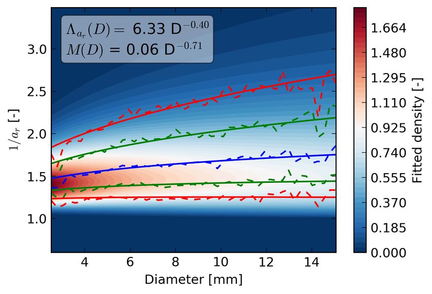
3890                   D. Wolfensberger and A. Berne: A forward polarimetric radar operator for the COSMO NWP model

                                                                            where wj0 = σ wj , wk0 = σ wk and zj0 = σ zj , zk0 = σ zk with
                                                                            σ = 2√123log
                                                                                      dB
                                                                                         2
                                                                                           , where 13 dB is the 3 dB beamwidth of the an-
                                                                            tenna in degrees. wj and zj are respectively the weights
                                                                            and the roots of the Hermite polynomial of order K (for
                                                                            elevational integration) and wk and zk are the weights and
                                                                            roots of the Hermite polynomial of order K (for azimuthal
                                                                            integration). For the integration in the radar operator, de-
                                                                            fault values of J = 5 and K = 7 are used according to Zeng
                                                                            et al. (2016). The quadrature points thus correspond to sep-
                                                                            arate sub-beams with different azimuth and elevation angles
Figure 3. Beam broadening increases the sampling volume with in-
                                                                            that are resolved independently. A schematic example of this
creasing range and is caused by the fact that the normalized power
                                                                            quadrature scheme is shown in Fig. 3 for J, K = 3.
density pattern of the antenna (shown in red/blue tones) is not com-
pletely concentrated on the beam axis. The blue dots correspond to             Another advantage of using a quadrature scheme is that is
the integration points used in the quadrature scheme (in this case          makes it easy to consider partial beam-blocking (grayed out
with J, K = 3 for illustration purposes) and their size depends on          area in Fig. 3). Note that in our operator, the blocked sub-
their corresponding weights. The effect of atmospheric refraction           beams are simply lost (i.e., are not considered in the integra-
on the propagation of the radar beam is also illustrated: r is the          tion) and no modeling of ground echoes is performed. How-
radial distance (radar range), s is the ground distance, and h the          ever, as was done in the evaluation of the operator (Sect. 4),
distance above ground of a given radar gate, which need to be esti-         these beams can easily be identified and removed when com-
mated accurately.                                                           paring simulated radar observables with real measurements.
                                                                               The choice of this simple Gaussian quadrature was vali-
       f 4 (θ0 − θ, φ0 − φ)|W (r0 − r)|2 cos θ drdθ dφ                (7)   dated by comparison with an exhaustive integration scheme
                                                                            during three precipitation events (two stratiform and one con-
   In our operator, similarly to Caumont et al. (2006)                      vective). The exhaustive integration consists in the decom-
and   Zeng et al. (2016), we set W (r0 − r) = 1 if r ∈                     position of a real antenna pattern (obtained from lab mea-
 r0 − cτ4 , r0 + cτ4 and W (r0 −r) = 0 otherwise. Indeed since

                                                                            surements) into a regular grid of 200 × 200 sub-beams. Such
the model resolution (1–2 km) is about one order of magni-                  an integration is obviously extremely computationally ex-
tude larger than the typical gate length of a modern radar                  pensive and can not be considered as a reasonable choice
(80–250 m), effects related to the finite receiver bandwidth                of quadrature in practice. Four other quadrature schemes
can be neglected. Integration over r can still be done a poste-             were tested, (1) a sparse Gauss–Hermite quadrature scheme
riori by using a higher radial resolution and aggregating the               (Smolyak, 1963), (2) a custom hybrid Gauss–Hermite and
simulated radar observables afterwards.                                     Legendre quadrature scheme based on the decomposition
   Another often used simplification is to neglect side lobes               of the real antenna diagram in radial direction with a sum
in the power density pattern and to approximate f 2 by a                    of Gaussians, (3) a Gauss–Legendre quadrature scheme
circularly symmetric Gaussian. These simplifications reduce                 weighted by the real antenna pattern, and (4) a recursive
the integration to Eq. (8).                                                 Gauss–Lobatto scheme (Gautschi, 2006) based on the real
                                                                            antenna pattern. All schemes were tested in terms of bias
                                                                          and root-mean-square-error (RMSE) in horizontal reflectiv-
I y (ro , θo , φo ) =                                                       ity ZH and differential reflectivity ZDR as a function of beam
       θo +π/2
          Z    φoZ+π                                            2         elevation (from 0 to 90◦ ), taking the exhaustive integration
                                                        θ0 − θ
                       y(r0 , θ, φ) exp −8 log 2                            scheme as a reference. Figure 4 shows an example for one
                                                        13 dB               of the two stratiform events. It was observed that the sim-
       θo −π/2 φo −π
                              2 !                                         ple Gauss–Hermite scheme was the one which performed
                φ0 − φ                                                      the best on average (lowest bias and RMSE for both ZH and
       −8 log 2                       cos θ dθ dφ                     (8)
                13 dB                                                       ZDR ), with schemes (1) and (3) performing almost system-
                                                                            atically worse. Schemes (2) and (4) tend to perform slightly
  This integration can be accurately approximated with a                    better at low elevation angles in particular situations where
Gauss–Hermite quadrature (Caumont et al., 2006):                            strong vertical gradients are present, generated for instance
                                                                            by a melting layer or by strong convection. This is due to
                      J
                      X                                                   the fact that in these situations, the contribution of the side
                        wj0 cos θ0 + zj0

I y (ro , θo , φo ) ≈                                                       lobes can become quite important, for example when the
                        j =1                                                main beam is located in the solid precipitation above the
       K
       X                                                                    melting layer but the first side lobe shoots through the melt-
             wk0 y(r0 , θ0 + zj0 , φ0 + zk0 ),                        (9)   ing layer or the rain underneath. However, considering that
       k=1

Atmos. Meas. Tech., 11, 3883–3916, 2018                                                       www.atmos-meas-tech.net/11/3883/2018/
D. Wolfensberger and A. Berne: A forward polarimetric radar operator for the COSMO NWP model 3891
8 April 2014 (stratiform)
1.6
1.4 Gaussian
Sparse Gaussian
1.2
RMSE in ZH [dBZ]
Multi. Gaussian
1.0
GL with real antenna
0.8 Rec. Lobatto
0.6
0.4
0.2
0.0
1.4
1.2
1.0
0.8 Figure 5. The direction of the far-field scattered wave is given by
Bias in ZH [dBZ]
0.6
the spherical angles θs and φs , or by the unit vector ψ̂ s . In the FSA
convention, the horizontal and vertical unit vectors are defined as
0.4 ĥs = φ̂s and v̂ s = φ̂s . The unit vectors for the spherical coordinate
0.2 system form the triplet (ψ̂ s , θ̂s , φ̂s ), which in the FSA convention
becomes (ψ̂ s , v̂ s , ĥs ), with ψ̂ s = v̂ s × ĥs . This figure was adapted
0.0
from Bringi and Chandrasekar (2001).
0.2
0.4
0 20 40 60 80 100
Elevation angle [°] The scattering matrix SFSA is a 2 × 2 matrix of complex
numbers in units of m−1 (e.g., Bringi and Chandrasekar,
Figure 4. Bias and RMSE in terms of ZH during one day of strati-
2001; Doviak and Zrnić, 2006; Mishchenko et al., 2002).
form of precipitation (around 120 RHI scans), for the five possible
quadrature schemes. The exhaustive quadrature scheme is used as a
reference. The other two events show similar results.
s shv
SFSA = hh (11)
svh svv FSA
these schemes are more computationally expensive and tend
The FSA subscript indicates the forward scattering align-
to perform worse at elevations > 3◦ , it was decided to keep
ment convention, in which the positive z-axis is in the same
the simple Gauss–Hermite scheme, which seems to offer the
direction as the travel of the wave (for both the incident and
best trade-off. However, as an improvement to the operator, it
scattered wave). A sketch illustrating the reference unit vec-
could be possible to use an adaptive scheme that depends on
tors for the scattered wave in the FSA convention is given in
the specific state of the atmosphere and the beam elevation.
Fig. 5.
In the FSA convention, the scattering matrix is also called
3.5 Derivation of polarimetric variables the Jones matrix (Jones, 1941). In the following the coef-
ficients of the backscattering matrix (scattering towards the
The mathematical formulation of the radar observables in- radar) will be denoted by s b , and the coefficients of the for-
volves the scattering matrix S, which relates the scattered ward scattering matrix (scattering away from the radar) by
electric field Es to the incident electric field Ei (Bringi and sf.
Chandrasekar, 2001) for a given scattering angle. All radar observables for a simultaneous transmitting radar
can be defined in terms of a backscattering covariance matrix
Cb and a forward scattering vector S f . For a given hydrome-
teor of type (j ) and diameter D.
Esh e−ik0 r
i
E
= SFSA hi , (10)
Esv r Ev
b,(j ) ∗
b,(j ) b,(j )
|shh |2 svv shh
Cb,(j ) (D) = b,(j ) b,(j ) ∗ b,(j )
∈ R2×2 , (12)
where k0 is the wave number of free space (k0 = 2π/λ). shh svv |svv |2
www.atmos-meas-tech.net/11/3883/2018/ Atmos. Meas. Tech., 11, 3883–3916, 20183892 D. Wolfensberger and A. Berne: A forward polarimetric radar operator for the COSMO NWP model
and In order to make the overall computation time reason-
able, the scattering properties for the individual hydrome-
" # teors are pre-computed for various common radar frequen-
f,(j )
f,(j ) shh cies and stored in three-dimensional lookup tables: diam-
S (D) = f,(j ) ∈ C 2×1 , (13)
svv eter, elevation and temperature for dry hydrometeors and
diameter, elevation and wet fraction for wet hydrometeors
where the superscripts b and f indicate backward, respec- (Sect. 3.7). On run time, these scattering properties are then
tively forward scattering directions and s are elements of the simply queried from the lookup tables, for a given elevation
scattering matrix SFSA (Eq. 11) that relates the scattered elec- angle and temperature and wet fraction.
tric field to the incident electric field for a given particle of
diameter D. 3.6.1 Aspect-ratios and orientations
The radar backscattering cross sections σ b are easily ob-
tained from Cb : Rain
For liquid precipitation (raindrops), the aspect-ratio model
b,(j ) b,(j )
σh (D) = 4π C1,1 (D) of (Thurai et al., 2007) is used and the drop orientation us
b,(j ) assumed to be normally distributed with a zero mean and
σvb,(j ) (D) = 4π C2,2 (D). (14)
a standard deviation of 7◦ according to Bringi and Chan-
All polarimetric variables at the radar gate polar coordi- drasekar (2001).
nates (ro , θo , φo ) are function of Cb and S f and can be ob-
tained by first integrating these scattering properties over the Snow and graupel
particle size distributions, summing them over all hydrom-
eteor types and finally integrating them over the antenna For solid precipitation, estimation of these parameters is a
power density. The exhaustive mathematical formulation of much more arduous task, since solid particles have a very
all simulated radar observables is given in Appendix C. Ad- wide variability in shape. Few aspect-ratio models have been
ditionally, real radar observations of ZH and ZDR are affected reported in the literature and even less is known about the
by attenuation, which needs to be accounted for to simulate orientations of solid hydrometeors.
realistic radar measurements. The specific differential phase In terms of aspect-ratio, Straka et al. (2000) report values
shift on propagation Kdp also needs to be modified in order ranging between 0.6 and 0.8 for dry aggregates and between
to account for the specific phase shift on backscattering (see 0.6 and 0.9 for graupel while Garrett et al. (2015) reports a
Appendix C). median aspect-ratio of 0.6 for aggregates and a strong mode
in graupel aspect-ratios around 0.9.
3.6 Scattering properties of individual hydrometeors In terms of orientation distributions, both Ryzhkov et al.
(2011) and Augros et al. (2016) consider a Gaussian distri-
Estimation of Cb,(j ) and S f,(j ) for individual hydrometeors bution with zero mean and a standard deviation of 40◦ for
is performed with the transition-matrix (T-matrix) method. aggregates and graupel in their simulations.
The T-matrix method is an efficient and exact generalization Given the large uncertainty associated with the geom-
of Mie scattering by randomly oriented nonspherical parti- etry of solid hydrometeors, a parameterization of aspect-
cles (Mishchenko et al., 1996). Since the shape of raindrops ratios and orientations for graupel and aggregates was de-
is widely accepted to be well approximated by spheroids rived using observations from a multi-angle snowflake cam-
(e.g., Andsager et al., 1999; Beard and Chuang, 1987; Thu- era (MASC). A detailed description of the MASC can be
rai et al., 2007), the T-matrix method provides a well suited found in Garrett et al. (2012). MASC observations recorded
method for the computation of the scattering properties of during one year in the Eastern Swiss Alps were classified
rain. This method was also used for the solid hydrometeors with the method of Praz et al. (2017), giving a total of around
(snow, graupel, hail and ice crystals), at the expense of some 30 000 particles for both hydrometeor types. The particles
adjustments, that will be described later on. were grouped into 50 diameter classes and inside every class
The T-matrix method requires knowledge about the per- a probability distribution was fitted for the aspect-ratio and
mittivity, the shape as well as the orientation of particles. the orientations. For sake of numerical stability, the fit was
Since particles are assumed to be spheroids, the aspect-ratio done on the inverse of the aspect-ratio (large dimension over
ar , defined in the context of this work as the ratio between small dimension). In accordance with the microphysical pa-
the smallest dimension and the largest dimension of a parti- rameterization of the model, the considered reference for the
cle, is sufficient to characterize their shapes. The orientation diameter of solid hydrometeors is their maximum dimension.
o is defined as the angle formed between the horizontal and The inverse of aspect ratio, 1/ar , is assumed to follow a
the major axis (canting angle ∈ [−90, 90]) and can be char- gamma distribution, whereas the canting angle o is assumed
acterized with the Euler angle β (pitch). to be normally distributed with zero mean, and the parame-
Atmos. Meas. Tech., 11, 3883–3916, 2018 www.atmos-meas-tech.net/11/3883/2018/D. Wolfensberger and A. Berne: A forward polarimetric radar operator for the COSMO NWP model 3893
ters of these distributions depend on the considered diameter q10 / q90 Observed (MASC)
q25 / q75
bin bDc. q50 (median) Model fit
(a)
o : go (o, D) = N (0, σo (D)) , (15)
1
ar −1
( a1r − 1)3ar (D)−1 exp − M(D)
1
: g1/ar (1/ar , D) = b, (16)
ar M(D)3ar (D) 0(3ar (D))
where 3ar and M are the shape and scale parameters of the
gamma aspect-ratio probability density function and σo is the
standard deviation of the Gaussian canting angle distribu-
tion. These parameters depend on the diameter D. Techni-
cally 3, M and σo have been fitted separately for each single
diameter bin of MASC, then their dependence on D has been (b)
fitted by power-laws for each parameter, which also allows
further integration over the canting angle and aspect-ratio
distributions for all particle sizes. Note also that the gamma
distribution is rescaled with a constant shift of 1, to account
for the fact that the smallest possible inverse of aspect-ratio
is 1 and not 0.
σo (D) = 58.07 D −0.11
◦
3ar (D) = 6.33 D −0.4 [−]
M(D) = 0.06 D −0.71 [−] (17)
Note that using the properties of the inverse distribution, Figure 6. Fitted probability density functions for the inverse of the
the distribution of aspect-ratios can easily be obtained from aspect-ratio (a) and the canting angle (b). The power-laws relat-
the distributions of their inverses: ing the particle density function parameters to the diameter are dis-
played in the grey boxes on the top-left. Note that the fit was per-
formed on the inverse of the aspect-ratio (major axis over minor
1 axis).
gar (ar , D) = g1/ar (1/ar , D). (18)
ar2
Figure 6 shows the fitted densities for every diameter and
every value of inverse aspect-ratio and canting angle. Over-
laid are the empirical quantiles (dashed lines) and the quan- less compact) and therefore the permittivity computed with
tiles of the fitted distributions (solid lines). Generally the the mixture model decreases as well. When the concentra-
match is quite good. The fitted models are able to take into tion increases, the proportion of larger (and more oblate)
account the increase in aspect-ratio spread and decrease in snowflakes increases but given their smaller permittivity, the
canting angle spread with particle size, which are the two overall trend is a slight decrease in ZDR . This trend hence re-
dominant trends that can be identified in the observations. flects an assumption in COSMO, not necessarily the reality.
Figure 7 shows the effect of using this MASC-based Note that even if this increase in the polarimetric signature
parameterization instead of the values from the literature of aggregates and graupel seems particularly drastic, com-
(Ryzhkov et al., 2011) on the resulting polarimetric vari- parisons with real radar measurements indicate that the op-
ables. Whereas only a small increase is observed for the hor- erator is still underestimating the polarimetric variables in
izontal reflectivity ZH , the difference is quite important for snow (Sect. 4.3).
ZDR and Kdp , especially for graupel. The MASC parame-
terization tends to produce a stronger polarimetric signature.
Hail
It is interesting to notice that ZDR tends to decrease with
the mass concentration, which is rather counter-intuitive as
ZDR is thought to be independent of concentration effects. A similar analysis could not be performed for hail, as no
This can be explained by the fact that, in COSMO, the den- MASC observations of hail were available. Hence, the cant-
sity of snowflakes decreases with their size (they become ing angle distribution is assumed to be Gaussian with zero
www.atmos-meas-tech.net/11/3883/2018/ Atmos. Meas. Tech., 11, 3883–3916, 20183894 D. Wolfensberger and A. Berne: A forward polarimetric radar operator for the COSMO NWP model
Permittivities
40 In the following, the term (complex) permittivity will be used
for the relative dielectric constant of a given material. It is
ZH [dBZ]
defined as follows:
20
0 = 0 + i 00 , (20)
where 0 is the real part, related to the phase velocity of the
propagated wave, and 00 is the imaginary part, related to the
0.015 absorption of the incident wave.
Rain
ZDR [dB]
0.010
For the permittivity of rain r , the well known model of Liebe
0.005 et al. (1991) for the permittivity of water at microwave fre-
quencies is used. Note that recently, a new model for water
0.000
permittivity has been proposed by Turner et al. (2016), which
appears to provide a better agreement with field observa-
tions at high frequencies. However, for common precipitation
1.5
radar frequencies (< 30 GHz) and temperatures (> −20◦ )
Kdp [ km 1]
both models agree very well.
1.0
Snow, graupel, hail and ice crystals
0.5
The permittivity of composite materials, such as snow, which
0.0 consists of a mixture of air and ice, can be estimated with a
10 5 10 4 10 3 10 2
so-called Effective Medium Approximation (EMA). A well
Concentration [g m 3] known EMA is the Maxwell–Garnett approximation (Bohren
and Huffman, 1983), in which the effective medium consists
Figure 7. Polarimetric variables at X-band (9.41 GHz) as a func- of a matrix medium with permittivity mat and inclusions
tion of the mass concentration for snow and graupel when using with permittivity inc :
canting angle and aspect-ratio parameterizations from the literature
(Ryzhkov et al., 2011) (solid line) and when using the parameteri- inc inc − mat
1 + 2fvol inc
+2 mat
zation based on MASC data (dashed line). eff = mat , (21)
inc inc − mat
1 − fvol inc +2 mat
where eff is the effective permittivity of the composite ma-
mean and a standard deviation of 40◦ , while the aspect-ratio inc is the volume fraction of the inclusions.
terial, and fvol
model is taken from (Ryzhkov et al., 2011). Note that other EMAs exist, such as the Bruggemann
(1935) and Oguchi (1983) approximations. If none of the
components is a strong dielectric, all these EMAs approxi-
mately agree to first order (Bohren and Huffman, 1983). The
1 − 0.02D,
if D < 10mm interested reader is referred to Blahak (2016), for an inter-
arhail = 0.8, if D ≥ 10mm (19) comparison of these EMA in the context of simulated reflec-
tivity fields.
Dry solid hydrometeors consist of inclusions of ice in a
matrix of air. In this case mat ≈ 1, which leads to a simplified
Ice crystals form of the mixing formula (e.g., Ryzhkov et al., 2011).
For ice-crystals, the aspect-ratio model is taken from Auer ice
ice −1
1 + 2fvol ice +2
and Veal (1970) for hexagonal columns, while the canting (j )
= , (22)
ice
ice −1
angle distribution is assumed to be Gaussian with zero mean 1 − fvol ice +2
and a standard deviation of 5◦ , which corresponds to the up-
per range of the canting angle standard deviations observed ice is the volume fractions of ice within the given
where fvol
by Noel and Sassen (2005) in cirrus and midlevel clouds. hydrometeor (snow, graupel or hail) and ice is the com-
Atmos. Meas. Tech., 11, 3883–3916, 2018 www.atmos-meas-tech.net/11/3883/2018/D. Wolfensberger and A. Berne: A forward polarimetric radar operator for the COSMO NWP model 3895
plex permittivity of ice, which can be estimated with Hufford where G is the overall radar gain in dBm, S is the radar an-
(1991)’s formula. tenna sensitivity in dBm, ZH is the horizontal reflectivity fac-
The densities ρ (j ) can be easily obtained from the tor in dBZ, and SNRthr corresponds to the desired signal-to-
(j ) D (b)
COSMO mass–diameter relations ρ (j ) = aπ/6D 3 and the noise threshold in dB (typically 8 dB in the following). r0 is
a distance used to normalize the argument of the logarithm.
density of ice is assumed to be constant ρi = 916 kg m−3 .
If all units are consistent then r0 = 1.
3.6.2 Integration of scattering properties
3.7 Simulation of the melting layer effect
The matrices Cb,(j ) (D) (Eq. 12) and S f,(j ) (D) (Eq. 13) are
obtained by integration over distributions of canting angles Stratiform rain situations are generally associated with the
and, for snow and graupel, aspect-ratios. For Cb,(j ) this gives presence of a melting layer (ML), characterized by a strong
the following for snow and graupel: signature in polarimetric radar variables (e.g., Szyrmer and
Zawadzki, 1999; Fabry and Zawadzki, 1995; Matrosov,
2008; Wolfensberger et al., 2016). In order to simulate re-
Cb,(j ) (D) = alistic radar observables, this effect needs to be taken into
Z2π Zπ/2 Z1 account by the radar operator. Unfortunately COSMO does
1
cb,(j ) (D, ar , α, o) cos(o) go (o, D) not operationally simulate wet hydrometeors, even though
2π a non-operational parameterization was developed by Frick
0 −π/2 0
and Wernli (2012). Jung et al. (2008) proposed a method
gar (ar , D) dα do dar , (23) to retrieve the mass concentration of wet snow aggregates
by considering co-existence of rain and dry hydrometeors as
and for rain and hail, where ar is constant for a given diame- an indicator of melting. A certain fraction of rain and dry
ter: snow is then converted to wet snow, which shows interme-
Z2π Zπ/2 diate properties between rain and dry snow, depending on
b,(j ) 1 the fraction of water within (wet fraction). As a first try to
C (D) = cb,(j ) (D, α, o) cos(o) go (o, D) dα do, (24)
2π simulate the melting layer we have implemented the method
0 −π/2
of Jung et al. (2008) and adapted it to also consider wet
where cb,(j ) (D, α, o) are the scattering properties for a fixed graupel. However, two issues with this method have been
diameter, canting angle o, and yaw Euler angle (azimuthal observed. First of all the co-existence of liquid water and
orientation) α. go (o) and gar are the probabilities of o and ar wet hydrometeors causes a secondary mode in the Doppler
for a given diameter D as obtained from Eqs. (15) and (18). spectrum within the melting layer, due to the different termi-
Note that the final scattering properties are averaged over all nal velocities, a mode that was never observed in the corre-
azimuthal angles α, which are all considered to be equiprob- sponding radar measurements. Secondly, the splitting of the
able. The cos(o) in the equation is the surface element which total mass into separate hydrometeor classes (rain and wet
arises from the fact that the integration over α and o is a sur- hydrometeors) causes an unrealistic decrease in reflectivity
face integration in spherical coordinates. The procedure for just underneath the melting layer. It was thus decided to use
S f is exactly the same. an alternative parameterization in which only wet aggregates
Since the computation of the T-matrix for a large number and wet graupel exist within the melting layer. At the bottom
of canting angles and aspect-ratios can be quite expensive, of the melting layer, where the wet fraction is usually almost
two different quadrature schemes were used, one Gauss– equal to unity, these particle behave almost like rain and at
Hermite scheme for the integration over the Gaussian distri- the top of the melting layer, where the wet fraction is usually
butions of canting angles, and one recursive Gauss–Lobatto very small, these particles behave like their dry counterparts.
scheme (Gander and Gautschi, 2000) for the integration over Note that contrary to Frick and Wernli (2012), which explic-
aspect-ratios. itly consider separate prognostic variables for the meltwater
on snowflakes, our scheme is purely diagnostic and is meant
3.6.3 Taking into account the radar sensitivity to be used in post-processing, when the COSMO model has
been run without a parameterization for melting snow.
The received power at the radar antenna decreases with the
square of the range, which leads to a decrease of signal-to- 3.7.1 Mass concentrations of wet hydrometeors
noise ratio (SNR) with the distance. To take into account this
effect, all simulated radar variables at range rg are censored
The fraction of wet hydrometeor mass is obtained by con-
if
verting the total mass of rain and dry hydrometeors within
rg the melting layer into melting aggregates and melting grau-
ZH (rg ) < S + G + SNRthr + 20 · log10 , (25) pel.
r0
www.atmos-meas-tech.net/11/3883/2018/ Atmos. Meas. Tech., 11, 3883–3916, 2018You can also read