159 Ensemble of regional climate model projections for Ireland - Author: Paul Nolan, Irish Centre for High-End Computing and Meteorology and ...
←
→
Page content transcription
If your browser does not render page correctly, please read the page content below
Report No. 159

Ensemble of regional climate model
             projections for Ireland
  Author: Paul Nolan, Irish Centre for High-End Computing
           and Meteorology and Climate Centre, School of
        Mathematical Sciences, University College Dublin

                                    www.epa.ie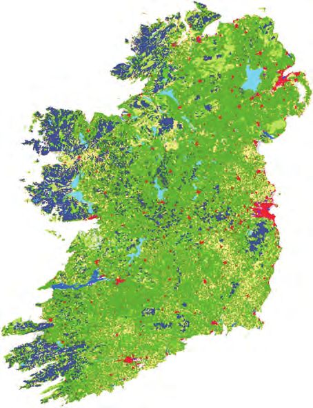
ENVIRONMENTAL PROTECTION AGENCY                                               Monitoring, Analysing and Reporting
The Environmental Protection Agency (EPA) is responsible for                  on the Environment
protecting and improving the environment as a valuable asset                  • Monitoring air quality and implementing the EU Clean Air
for the people of Ireland. We are committed to protecting                       for Europe (CAFÉ) Directive.
people and the environment from the harmful effects of                        • Independent reporting to inform decision making by
radiation and pollution.                                                        national and local government (e.g. periodic reporting on the
                                                                                State of Ireland’s Environment and Indicator Reports).
The work of the EPA can be
divided into three main areas:                                                Regulating Ireland’s Greenhouse Gas Emissions
                                                                              • Preparing Ireland’s greenhouse gas inventories and projections.
Regulation: We implement effective regulation and
environmental compliance systems to deliver good                              • Implementing the Emissions Trading Directive, for over 100
environmental outcomes and target those who don’t comply.                       of the largest producers of carbon dioxide in Ireland.

Knowledge: We provide high quality, targeted                                  Environmental Research and Development
and timely environmental data, information and                                • Funding environmental research to identify pressures,
assessment to inform decision making at all levels.                             inform policy and provide solutions in the areas of climate,
                                                                                water and sustainability.
Advocacy: We work with others to advocate for a
clean, productive and well protected environment                              Strategic Environmental Assessment
and for sustainable environmental behaviour.                                  • Assessing the impact of proposed plans and programmes on
                                                                                the Irish environment (e.g. major development plans).
Our Responsibilities
                                                                              Radiological Protection
Licensing
                                                                              • Monitoring radiation levels, assessing exposure of people in
We regulate the following activities so that they do not                        Ireland to ionising radiation.
endanger human health or harm the environment:
                                                                              • Assisting in developing national plans for emergencies arising
• waste facilities (e.g. landfills, incinerators, waste transfer stations);     from nuclear accidents.
• large scale industrial activities (e.g. pharmaceutical, cement              • Monitoring developments abroad relating to nuclear installations
  manufacturing, power plants);                                                 and radiological safety.
• intensive agriculture (e.g. pigs, poultry);                                 • Providing, or overseeing the provision of, specialist radiation
• the contained use and controlled release of Genetically                       protection services.
  Modified Organisms (GMOs);
• sources of ionising radiation (e.g. x-ray and radiotherapy                  Guidance, Accessible Information and Education
  equipment, industrial sources);                                             • Providing advice and guidance to industry and the public on
• large petrol storage facilities;                                              environmental and radiological protection topics.
• waste water discharges;                                                     • Providing timely and easily accessible environmental
                                                                                information to encourage public participation in environmental
• dumping at sea activities.                                                    decision-making (e.g. My Local Environment, Radon Maps).
National Environmental Enforcement                                            • Advising Government on matters relating to radiological
                                                                                safety and emergency response.
• Conducting an annual programme of audits and inspections
  of EPA licensed facilities.                                                 • Developing a National Hazardous Waste Management Plan to
                                                                                prevent and manage hazardous waste.
• Overseeing local authorities’ environmental
  protection responsibilities.                                                Awareness Raising and Behavioural Change
• Supervising the supply of drinking water by public water                    • Generating greater environmental awareness and influencing
  suppliers.                                                                    positive behavioural change by supporting businesses,
• Working with local authorities and other agencies                             communities and householders to become more resource
  to tackle environmental crime by co-ordinating a                              efficient.
  national enforcement network, targeting offenders and                       • Promoting radon testing in homes and workplaces and
  overseeing remediation.                                                       encouraging remediation where necessary.
• Enforcing Regulations such as Waste Electrical and
  Electronic Equipment (WEEE), Restriction of Hazardous                       Management and structure of the EPA
  Substances (RoHS) and substances that deplete the                           The EPA is managed by a full time Board, consisting of a Director
  ozone layer.                                                                General and five Directors. The work is carried out across five
• Prosecuting those who flout environmental law and damage                    Offices:
  the environment.                                                            • Office of Climate, Licensing and Resource Use
Water Management                                                              • Office of Environmental Enforcement
• Monitoring and reporting on the quality of rivers, lakes,                   • Office of Environmental Assessment
  transitional and coastal waters of Ireland and groundwaters;                • Office of Radiological Protection
  measuring water levels and river flows.                                     • Office of Communications and Corporate Services
• National coordination and oversight of the Water                            The EPA is assisted by an Advisory Committee of twelve
  Framework Directive.                                                        members who meet regularly to discuss issues of concern and
• Monitoring and reporting on Bathing Water Quality.                          provide advice to the Board.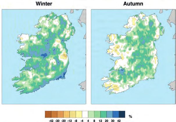
EPA Research Programme 2014–2020

Ensemble of regional climate model projections
                 for Ireland

                           (2008-FS-CC-m)

                 Prepared for the Environmental Protection Agency

                                        by

 Irish Centre for High-End Computing and Meteorology and Climate Centre, School of
                   Mathematical Sciences, University College Dublin

                                     Author:

                                   Paul Nolan

                ENVIRONMENTAL PROTECTION AGENCY
                 An Ghníomhaireacht um Chaomhnú Comhshaoil
               PO Box 3000, Johnstown Castle, Co. Wexford, Ireland

               Telephone: +353 53 916 0600 Fax: +353 53 916 0699
                     Email: info@epa.ie Website: www.epa.ie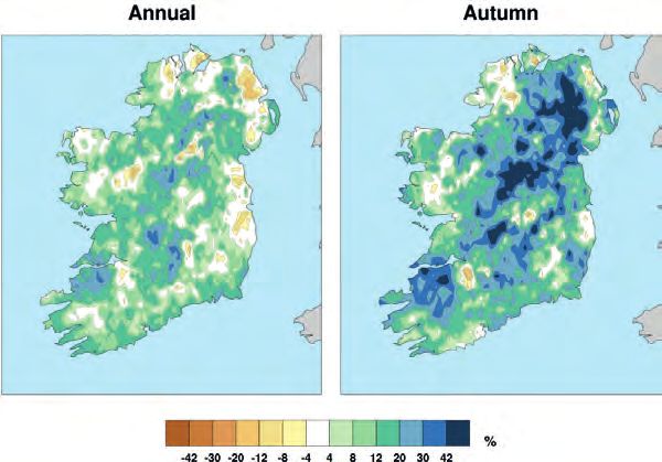
© Environmental Protection Agency 2015

                                ACKNOWLEDGEMENTS
The author wishes to acknowledge and thank the EPA for supporting and funding this research. In
particular, Margaret Desmond, Philip O’Brien and Frank McGovern are thanked for their helpful
input and support. The research was carried out at the Irish Centre for High-End Computing
(ICHEC) and the Meteorology and Climate Centre, University College Dublin (UCD).

We are grateful for the input of Ray McGrath of the Research and Applications Division, Met
Éireann, and Conor Sweeney and John O’Sullivan of the Meteorology and Climate Centre, UCD.
Seamus Walsh of Met Éireann is acknowledged for supplying the observed climate data. We are
thankful to Daniel Purdy of ICHEC/Trinity College Dublin for his assistance with the storm-
tracking analysis. Emily Gleeson of Met Éireann is also acknowledged. Finally, Professor Peter
Lynch of the Meteorology and Climate Centre, UCD, is thanked for his supervision and support
while the author worked at UCD.

The author wishes to acknowledge ICHEC for the provision of computational facilities and
support. All simulations of the study were carried out on the ICHEC supercomputing facilities
(funded by Science Foundation Ireland).

                                        DISCLAIMER
Although every effort has been made to ensure the accuracy of the material contained in this
publication, complete accuracy cannot be guaranteed. Neither the Environmental Protection
Agency nor the author(s) accept any responsibility whatsoever for loss or damage occasioned
or claimed to have been occasioned, in part or in full, as a consequence of any person acting or
refraining from acting, as a result of a matter contained in this publication. All or part of this
publication may be reproduced without further permission, provided the source is acknowledged.

The EPA Research Programme addresses the need for research in Ireland to inform policymakers
and other stakeholders on a range of questions in relation to environmental protection. These
reports are intended as contributions to the necessary debate on the protection of the environment.

                     EPA RESEARCH PROGRAMME 2014–2020
                    Published by the Environmental Protection Agency, Ireland

                               PRINTED ON RECYCLED PAPER

ISBN: 978-1-84095-609-2

Price: Free                                                                              10/15/150

                                                 ii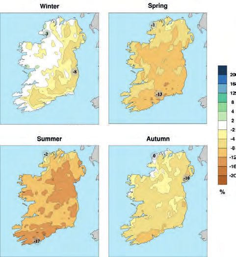
Project partner

Dr Paul Nolan
Irish Centre for High-end Computing
Trinity Technology and Enterprise Campus
Grand Canal Quay
Dublin 2
and formerly of the Meteorology and Climate Centre
School of Mathematical Sciences
University College Dublin
Belfield
Dublin 4
Tel.: +353 1 5241608 (ext. 32)
E-mail: paul.nolan@ichec.ie

                                             iii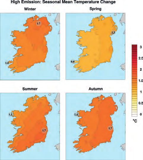
Contents

Executive summary                                                                      xiii

1      Introduction                                                                      1

        1.1    Regional climate models                                                   1

        1.2    Downscaling to Ireland                                                    1

        1.3    Regional climate model evaluation                                         3

        1.4    Greenhouse gas emission scenarios                                         4

        1.5    Regional climate model projections                                        4

        1.6    Overview of uncertainty                                                   5

        1.7    Statistical significance analysis                                         6

        References7

2      Impacts of climate change on Irish temperature                                    9

        2.1    Introduction                                                              9

        2.2    Regional climate model temperature validations                           11

        2.3    Temperature projections for Ireland                                      11

        2.4    Conclusions                                                              25

        References25

3      Impacts of climate change on Irish precipitation                                 27

        3.1    Introduction                                                             27

        3.2    Regional climate model precipitation validations                         29

        3.3    Precipitation projections for Ireland                                    30

        3.4    Conclusions                                                              41

        References42

4      Impacts of climate change on Irish wind energy resource                          44

        4.1    Introduction                                                             44

        4.2    Regional climate model wind validations                                  46

        4.3    Wind projections for Ireland                                             51

        4.4    Projected changes in extreme storm tracks and mean sea-level pressure    60

        4.5    Conclusions                                                              64

        References66

Abbreviations68

                                                           v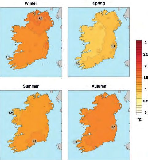
List of figures

Figure 1.1.   The WRF model domains. The d01, d02 and d03 domains have 54-km, 18-km and 6-km horizontal
              resolution, respectively                                                                             2

Figure 1.2.   The topography of Ireland and the UK as resolved by the EC-Earth GCM and the CLM RCM for
              different spatial resolutions. (a) EC-Earth 125-km resolution; (b) CLM 50-km resolution; (c) CLM
              18-km resolution; (d) CLM 4-km resolution                                                            2

Figure 1.3.   A schematic diagram of the probability density function of the ensemble of projected changes in
              temperature. The red vertical line shows the likely increase in temperature                          5

Figure 1.4.   Distributions of past and future temperature data. (a) Cumulative density function; (b) probability
              density function                                                                                     6

Figure 2.1.   Annual 2-m temperature for the period 1981–2000. (a) Observations; (b) CLM-ERA 4 km data;
              (c) CLM-ERA minus observations (bias)                                                                11

Figure 2.2.   Seasonal 2-m temperature for 1981–2000. The first, second and third columns contain observations,
              CLM-ERA data and the bias, respectively. The colour scale is kept fixed for each column and is
              included in the last row                                                                             12

Figure 2.3.   Annual mean temperature anomalies for each of the five emission scenarios, averaged across every
              grid point over Ireland. (a) Time series of the annual mean temperature anomalies. The dashed coloured
              lines are lines of regression fitted using the least-squares method. (b) Seasonal mean temperature
              anomalies for winter (December–February), spring (March–May), summer (June–August) and
              autumn (September–November). The boxplots represent the spread of each group; the bottom and
              top whiskers represent the minimum and maximum group values, respectively, the bottom and top
              of the box represent the group’s first and third quartiles, respectively, and the middle line represents
              the group’s median. For both figures, the future period 2041–2060 is compared with the past period
              1981–200013

Figure 2.4.   Projected changes in annual mean temperature for the (a) medium- to low-emission and (b) high-
              emission scenarios. In each case, the future period 2041–2060 is compared with the past period
              1981–2000. The numbers included on each plot are the minimum and maximum projected changes,
              displayed at their locations                                                                         14

Figure 2.5.   Projected changes in seasonal mean temperature for the (a) medium- to low-emission and (b) high-
              emission scenarios. In each case, the future period 2041–2060 is compared with the past period
              1981–200014

Figure 2.6.   The “very likely” annual increase in temperature for the (a) medium- to low-emission and (b) high-
              emission scenarios. In each case, the future period 2041–2060 is compared with the past period
              1981–2000. The numbers included on each plot are the minimum and maximum “very likely”
              increases, displayed at their locations                                                              15

Figure 2.7.   The “very likely” seasonal increase in temperature for the (a) medium- to low-emission and (b) high-
              emission scenarios. In each case, the future period 2041–2060 is compared with the past period
              1981–200016

                                                           vi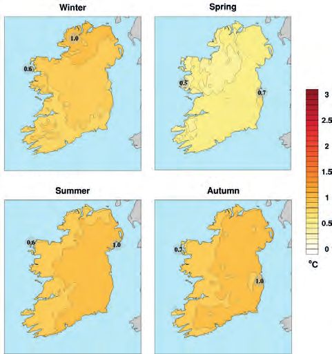
List of figures

Figure 2.8.    The “likely” annual increase in temperature for the (a) medium- to low-emission and (b) high-emission
               scenarios. In each case, the future period 2041–2060 is compared with the past period 1981–2000.
               The numbers included on each plot are the minimum and maximum “likely” increases, displayed at
               their locations                                                                                            16

Figure 2.9.    The “likely” seasonal increase in temperature for the (a) medium- to low-emission and (b) high-
               emission scenarios. In each case, the future period 2041–2060 is compared with the past period
               1981–200017

Figure 2.10.   Projected changes in the top 5% of maximum daytime summer temperatures for the medium- to
               low-emission and high-emission scenarios. In each case, the future period 2041–2060 is compared
               with the past period 1981–2000. The numbers included on each plot are the minimum and maximum
               increases, displayed at their locations                                                                    17

Figure 2.11.   Projected changes in the lowest 5% of night-time winter temperatures for the medium- to low-
               emission and high-emission scenarios. In each case, the future period 2041–2060 is compared with
               the past period 1981–2000. The numbers included on each plot are the minimum and maximum
               increases, displayed at their locations                                                                    18

Figure 2.12.   Annual frost day statistics. (a) Projected percentage change in annual number of frost days for the
               medium- to low-emission and high-emission scenarios. In each case, the future period 2041–2060 is
               compared with the past period 1981–2000. (b) The observed mean annual number of frost days, over
               land, for 1981–2000                                                                                        18

Figure 2.13.   Annual ice day statistics. (a) Projected percentage change in annual number of ice days for the
               medium- to low-emission and high-emission scenarios. In each case, the future period 2041–2060 is
               compared with the past period 1981–2000. (b) The observed mean annual number of ice days, over
               land, for 1981–2000                                                                                        19

Figure 2.14.   Empirical density functions illustrating the distribution of past (black), medium- to low-emission (blue)
               and high-emission (red) mean daily temperatures over Ireland. (a) Winter; (b) spring; (c) summer;
               (d) autumn. Each dataset has a size greater than 80 million. The distributions are created using
               histogram bins of size 0.5°C. A measure of overlap indicates how much the future distributions have
               changed relative to the past (0% indicating no common area, 100% indicating complete agreement).
               Means are shown for historical (black vertical line), medium- to low-emission (blue vertical line) and
               high-emission (red vertical line) densities                                                                20

Figure 2.15.   Seasonal projected changes in the standard deviation of mean daily temperature. (a) Medium- to
               low-emission ensemble; (b) high-emission ensemble. In each case, the future period 2041–2060 is
               compared with the past period 1981–2000. The numbers included on each plot are the minimum and
               maximum projected changes, displayed at their locations                                                    21

Figure 2.16.   Annual projected changes in the standard deviation of mean daily temperature. (a) Medium- to low-
               emission scenario; (b) high-emission scenario. In each case, the future period 2041–2060 is compared
               with the past period 1981–2000                                                                             21

Figure 2.17.   The standard deviation of mean daily temperature for the past period 1981–2000. (a) Annual; (b) winter;
               (c) spring; (d) summer; (e) autumn. The figures were generated using all RCM ensemble member data
               for the control period. The numbers included on each plot are the minimum and maximum values,
               displayed at their locations                                                                               22

Figure 2.18.   Projected changes the length of the growing season (days per year). (a) Medium- to low-emission
               scenario; (b) high-emission scenario. In each case, the future period 2041–2060 is compared with the
               past period 1981–2000                                                                                      23

                                                               vii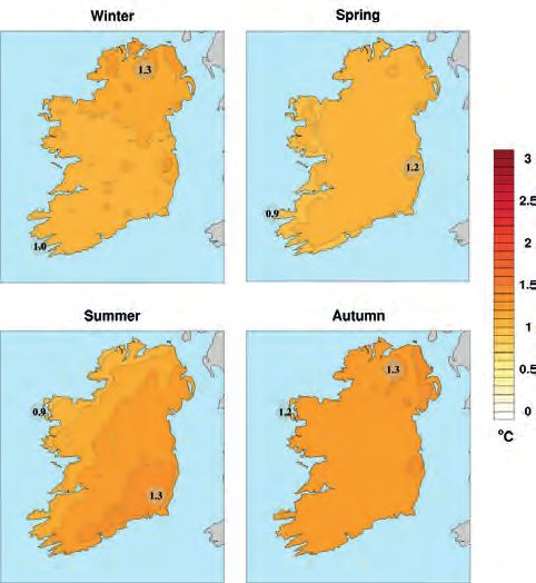
List of figures
Figure 2.19. Land use statistics. (a) Coordination of Information on the Environment (CORINE) land cover map
of Ireland. The colours represent the land cover in 2006. (Image reproduced with permission from
Dwyer, 2012.) (b) Observed annual length of growing season for the period 1981–2000. (Temperature
data from Walsh, 2012.) 23
Figure 2.20. “Very likely” increase in the length of the growing season (days per year). (a) Medium- to low-
emission scenario; (b) high-emission scenario. In each case, the future period 2041–2060 is compared
with the past period 1981–2000 24
Figure 2.21. “Likely” increase in the length of the growing season (days per year). (a) Medium- to low-emission
scenario; (b) high-emission scenario. In each case, the future period 2041–2060 is compared with the
past period 1981–2000 24
Figure 3.1. Mean annual precipitation for 1981–2000. (a) Observations; (b) CLM–EC-Earth 4-km data; (c) CLM–
EC-Earth minus observations (error) 27
Figure 3.2. Seasonal precipitation for 1981–2000. The first, second and third columns contain observations,
CLM–EC-Earth data and the error, respectively. The colour scale is kept fixed for each column and is
included in the last row 31
Figure 3.3. Annual and seasonal mean precipitation errors (%). (a) Overall bias; (b) overall MAE metrics. Each
RCM past ensemble member is compared with observations for the 20-year period 1981–2000.
The boxplots represent the spread of errors; the bottom and top whiskers represent the minimum
and maximum, respectively, the bottom and top of the box represents the first and third quartiles,
respectively, and the middle line represents the median error 32
Figure 3.4. Projected change (%) in annual precipitation. (a) Medium- to low-emission scenario; (b) high-emission
scenario. In each case, the future period 2041–2060 is compared with the past period 1981–2000. The
numbers included on each plot are the minimum and maximum changes, displayed at their locations 32
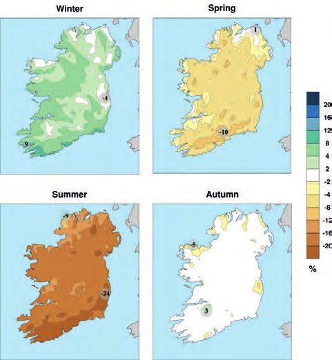
Figure 3.5. Projected changes (%) in seasonal precipitation. (a) Medium- to low-emission scenario; (b) high-
emission scenario. In each case, the future period 2041–2060 is compared with the past period
1981–200033
Figure 3.6. “Likely” change (%) in precipitation. (a) Annual; (b) spring. In each case, the future period 2041–2060
is compared with the past period 1981–2000 33
Figure 3.7. Projected change (%) in summer precipitation. (a) “Likely”; (b) “very likely”. In each case, the future
period 2041–2060 is compared with the past period 1981–2000 34
Figure 3.8. “Likely” change (%) in the number of dry periods. (a) Annual; (b) autumn. In each case, the future
period 2041–2060 is compared with the past period 1981–2000 34
Figure 3.9. Projected change (%) in number of summer dry periods. (a) “Likely”; (b) “very likely”. In each case,
the future period 2041–2060 is compared with the past period 1981–2000 35
Figure 3.10. The observed number of dry periods averaged over the 20-year period 1981–2000. (a) Annual;
(b) autumn; (c) summer. Note the different scale for the annual figure 35
Figure 3.11. The “likely” increase in number of winter and autumn wet days (rainfall > 20 mm) for the high-
emission scenario. In each case, the future period 2041–2060 is compared with the past period
1981–200036
Figure 3.12. The “likely” increase in number of annual and autumn very wet days (rainfall > 30 mm) for the
high-emission scenario. In each case, the future period 2041–2060 is compared with the past period
1981–200036
viiiList of figures
Figure 3.13. The observed number of wet days (rainfall > 20 mm) averaged over the 20-year period 1981–2000.
(a) Annual; (b) winter; (c) autumn. Note the different scale for the annual figure 37
Figure 3.14. The observed number of very wet days (rainfall > 30 mm) averaged over the 20-year period 1981–
2000. (a) Annual; (b) winter; (c) autumn. Note the different scale for the annual figure 37
Figure 3.15. Empirical density functions illustrating the distribution of past (black), medium- to low-emission
(blue) and high-emission (red) daily precipitation over Ireland. (a) Winter; (b) spring; (c) summer;
(d) autumn. Each dataset has a size greater than 80 million. The distributions are created using
histogram bins of size 1 mm. A measure of overlap indicates how much the future distributions have
changed relative to the past (0% indicating no common area, 100% indicating complete agreement).
Means are shown for historical (black vertical line), medium- to low-emission (blue vertical line) and
high-emission (red vertical line) densities 38
Figure 3.16. Empirical density functions illustrating the distribution of past (black), medium- to low-emission
(blue) and high-emission (red) daily precipitation over Ireland. (a) Annual; (b) annual with the
frequency displayed on a log scale. Each dataset has a size greater than 80 million. The distributions
are created using histogram bins of size 1 mm (a) and 4 mm (b) 39
Figure 3.17. Empirical density functions illustrating the distribution of past (black), medium- to low-emission
(blue) and high-emission (red) heavy precipitation over Ireland. (a) Autumn; (b) winter. The frequency
is displayed on a log scale. Each dataset has a size greater than 80 million. The distributions are
created using histogram bins of size 4 mm 39
Figure 3.18. Seasonal projected changes (%) in the standard deviation of daily precipitation. (a) Medium- to
low-emission ensemble; (b) high-emission ensemble. In each case, the future period 2041–2060 is
compared with the past period 1981–2000. The numbers included on each plot are the minimum and
maximum projected change, displayed at their location 40
Figure 3.19. Annual projected changes (%) in the standard deviation of daily precipitation. (a) Medium- to
low-emission ensemble; (b) high-emission ensemble. In each case, the future period 2041–2060 is
compared with the past period 1981–2000. The numbers included on each plot are the minimum and
maximum projected change, displayed at their locations 41
Figure 4.1. Comparing the observed 3-hourly 10-m winds at nine synoptic stations spanning Ireland with the
RCM ensemble members for the period 1981–2000. (a) Wind speed distribution; (b) wind speed
percentiles; (c) mean monthly wind speed; (d) mean diurnal cycle. The following RCM validation
datasets are considered: CLM3-ECHAM5 7 km (two ensemble members), CLM4-ECHAM5 7 km
(two ensemble members), WRF–EC-Earth 6 km (three ensemble members), CLM4-CGCM3.1 4 km
(one ensemble member), CLM4-HadGEM2-ES 4 km (one ensemble member), CLM4–EC-Earth 4 km
(three ensemble members) and the total RCM ensemble (12 members). For (c) and (d), the RCM
dataset means are considered 46
Figure 4.2. Annual 10-m wind roses at eight Met Éireann synoptic stations spanning Ireland. (a) Observed data;
(b) CLM4–EC-Earth 4-km data 47
Figure 4.3. Annual diurnal 10-m mean cubed wind speed, averaged over nine station locations for 1981–2000.
(a) Observation; (b) CLM3-ECHAM5 7 km (two ensemble members); (c) CLM4-ECHAM5 7 km
(two ensemble members); (d) WRF–EC-Earth 6 km (three ensemble members); (e) CLM4-CGCM3.1
4 km (one ensemble member); (f) CLM4-HadGEM2-ES 4 km (one ensemble member); (g) CLM4–
EC-Earth 4 km (three ensemble members); (h) RCM ensemble mean (12 members); (i) RCM ensemble
percentage error 48
ixList of figures
Figure 4.4. The 10-m wind roses at Casement Aerodrome for 1981–2000. (a) Observed; (b) WRF–EC-Earth
ensemble (three members) 6-km resolution; (c) WRF–EC-Earth ensemble (three members) 18-km
resolution. Each sector shows the percentage breakdown of the wind speed in intervals of 2 m/s 48
Figure 4.5. The 10-m wind power roses at Casement Aerodrome for 1981–2000. (a) Observed; (b) CLM4–
EC-Earth ensemble (three members) 4-km resolution; (c) CLM4–EC-Earth ensemble (three members)
18-km resolution. The wind power rose shows the directional frequency (light blue segments), the
contribution of each sector to the total mean wind speed (blue segments) and the contribution of each
sector to the total mean cube of the wind speed (red segments) 49
Figure 4.6. Winter 10-m wind roses at eight Met Éireann synoptic stations spanning Ireland. (a) Observed data;
(b) CLM4–EC-Earth 4-km data 49
Figure 4.7. Spring 10-m wind roses at eight Met Éireann synoptic stations spanning Ireland. (a) Observed data;
(b) CLM4–EC-Earth 4-km data 50
Figure 4.8. Summer 10-m wind roses at eight Met Éireann synoptic stations spanning Ireland. (a) Observed data;
(b) CLM4–EC-Earth 4-km data 50
Figure 4.9. Autumn 10-m wind roses at eight Met Éireann synoptic stations spanning Ireland. (a) Observed data;
(b) CLM4–EC-Earth 4-km data 50
Figure 4.10. Annual 10-m wind power roses at eight Met Éireann synoptic stations spanning Ireland. (a) Observed
data; (b) CLM4–EC-Earth 4-km data 51
Figure 4.11. Winter 10-m wind power roses at eight Met Éireann synoptic stations spanning Ireland. (a) Observed
data; (b) CLM4–EC-Earth 4-km data 51
Figure 4.12. Spring 10-m wind power roses at eight Met Éireann synoptic stations spanning Ireland. (a) Observed
data; (b) CLM4–EC-Earth 4-km data 52
Figure 4.13. Summer 10-m wind power roses at eight Met Éireann synoptic stations spanning Ireland. (a) Observed
data; (b) CLM4–EC-Earth 4-km data 52
Figure 4.14. Autumn 10-m wind power roses at eight Met Éireann synoptic stations spanning Ireland. (a) Observed
data; (b) CLM4–EC-Earth 4-km data 52
Figure 4.15. Ensemble projected change (%) in annual 60-m mean wind power. (a) Medium- to low-emission
scenario; (b) high-emission scenario. In each case, the future period 2041–2060 is compared with the
past period 1981–2000. The numbers included on each plot are the minimum and maximum changes,
displayed at their locations 53
Figure 4.16. Projected changes (%) in seasonal 60-m mean wind power. (a) Medium- to low-emission scenario;
(b) high-emission scenario. In each case, the future period 2041–2060 is compared with the past
period 1981–2000 53
Figure 4.17. “Likely” decrease in 60-m mean wind power. (a) Annual; (b) spring. In each case, the future period
2041–2060 is compared with the past period 1981–2000 54
Figure 4.18. Projected decrease in summer 60-m mean wind power. (a) “Likely”; (b) “very likely”. In each case,
the future period 2041–2060 is compared with the past period 1981–2000 55
Figure 4.19. Annual diurnal 60-m mean cubed wind speed over Ireland and a small portion of the surrounding
sea. (a) Ensemble of past simulations, 1981–2000; (b) ensemble of high-emission future simulations,
2041–2060; (c) projected percentage change 56
Figure 4.20. Wind roses at 60-m at various locations spanning Ireland. (a) Winter ensemble of past simulations,
1981–2000; (b) winter ensemble of high-emission future simulations, 2041–2060; (c) summer
xList of figures
ensemble of past simulations, 1981–2000; (d) summer ensemble of high-emission future simulations,
2041–206056
Figure 4.21. Wind power roses at 60-m at various locations spanning Ireland. (a) Winter ensemble of past
simulations, 1981–2000; (b) winter ensemble of high-emission future simulations, 2041–2060;
(c) summer ensemble of past simulations, 1981–2000; (d) summer ensemble of high-emission future
simulations, 2041–2060 57
Figure 4.22. Empirical density functions illustrating the distribution of past (black), medium- to low-emission
(blue) and high-emission (red) 60-m daily mean wind speed over Ireland. (a) Winter; (b) spring;
(c) summer; (d) autumn. Each dataset has a size greater than 80 million. The distributions are created
using histogram bins of size 1 m/s. A measure of overlap indicates how much the future distributions
have changed relative to the past (0% indicating no common area, 100% indicating complete
agreement). Means are shown for historical (black vertical line), medium- to low-emission (blue
vertical line) and high-emission (red vertical line) densities 58
Figure 4.23. Seasonal projected changes (%) in the standard deviation of daily mean 60-m wind speed. (a) Medium-
to low-emission ensemble; (b) high-emission ensemble. In each case, the future period 2041–2060 is
compared with the past period 1981–2000. The numbers included on each plot are the minimum and
maximum projected change, displayed at their locations 59
Figure 4.24. Annual projected changes (%) in the standard deviation of daily mean 60m wind speed. (a) Medium-
to low-emission ensemble; (b) high-emission ensemble. In each case, the future period 2041–2060 is
compared with the past period 1981–2000. The numbers included on each plot are the minimum and
maximum projected change, displayed at their locations 59
Figure 4.25. Empirical density functions illustrating the distribution of past (black), medium- to low-emission (blue)
and high-emission (red) 60-m daily maximum wind speeds over Ireland. (a) Winter; (b) annual. The
frequency is displayed on a log scale. Each dataset has a size greater than 80 million. The distributions
are created using histogram bins of size 1 m/s 60
Figure 4.26. Location of a local MSLP minimum. Here the point (i, j) is defined as a low-pressure centre, since all
MSLP values of the surrounding 80 grid points are greater than p(i, j) = 938 hPa 61
Figure 4.27. Tracks of storms with a core MSLP of less than 940 hPa and with a lifetime of at least 12 hours.
(a) Past RCM 18-km simulations (1981–2000); (b) RCP8.5 RCM 18-km simulations (2041–2060) 62
Figure 4.28. Tracks of storms with a core MSLP of less than 940 hPa and with a lifetime of at least 12 hours.
(a) Past RCM 50-km simulations (1981–2000); (b) RCP8.5 RCM 50-km simulations (2041–2060) 62
Figure 4.29. RCM average MSLP. (a) Past simulations (1981–2000); (b) RCP4.5 simulations (2041–2060);
(c) RCP8.5 simulations (2041–2060) 63
Figure 4.30. The “likely” increase in annual average MSLP for the RCP4.5 and RCP8.5 simulations. In each case,
the future period 2041–2060 is compared with the past period 1981–2000 63
Figure 4.31. The “likely” increase in winter average MSLP for the RCP4.5 and RCP8.5 simulations. In each case,
the future period 2041–2060 is compared with the past period 1981–2000 64
Figure 4.32. The “likely” increase in spring average MSLP for the RCP4.5 and RCP8.5 simulations. In each case,
the future period 2041–2060 is compared with the past period 1981–2000 64
Figure 4.33. The “likely” increase in summer average MSLP for the RCP4.5 and RCP8.5 simulations. In each
case, the future period 2041–2060 is compared with the past period 1981–2000 65
Figure 4.34. The “likely” increase in autumn average MSLP for the RCP4.5 and RCP8.5 simulations. In each case,
the future period 2041–2060 is compared with the past period 1981–2000 65
xiList of tables
Table 1.1. Output fields of the WRF simulations 3
Table 1.2. Details of the ensemble of RCM simulations 4
Table 1.3. Likelihood terms and their associated probabilities 5
Table 4.1. The RCM simulations used for the storm tracking and MSLP analysis 61
xiiExecutive summary
This report provides an analysis of the impacts of climate was simulated using the Intergovernmental
global climate change on the mid-21st-century climate Panel on Climate Change (IPCC) Special Report on
of Ireland. The projections are based on the output of Emissions Scenarios (SRES) A1B, A2 and B1 and the
an ensemble of high-resolution regional climate models Representative Concentration Pathways (RCP) 4.5 and
(RCMs). 8.5 (IPCC, Fifth Assessment Report) emission scenar-
ios. The RCP4.5 and the B1 scenario simulations were
The impact of rising greenhouse gas emissions and
used to create a “medium- to low-emission” ensemble
changing land use on climate can be simulated using
while the RCP8.5, A1B and A2 simulations were used
global climate models (GCMs). However, since GCMs
to create a “high-emission” ensemble. To address the
are computationally expensive to run, long climate
issue of uncertainty, a multi-model ensemble (MME)
simulations are currently feasible only with horizontal
approach was employed. Through the MME approach,
resolutions of 50 km or coarser. Since climate fields such
the uncertainty in RCM projections can be partially
as precipitation and wind speed are closely correlated
quantified, thus providing a measure of confidence in
with the local topography, this resolution is inadequate
the predictions.
for the simulation of the detail and pattern of climate
change on the scale of a region the size of Ireland. To The RCMs were validated using 20-year simulations
overcome this limitation, the RCM method dynamically of the past Irish climate (1981–2000), driven both
downscales the coarse information provided by the by European Centre for Medium-Range Weather
global models and provides high-resolution information Forecasts (ECMWF) ERA-40 global re-analysis and the
on a subdomain covering Ireland. The computational GCM datasets and by comparing the output against Met
cost of running the RCM, for a given resolution, is con- Éireann observational data. Extensive validations were
siderably less than that of a global model. The RCMs carried out to test the ability of the RCMs to accurately
of the current study were run at high spatial resolution, model the climate of Ireland. Results confirm that the
up to 4 km, thus allowing a better evaluation of the local output of the RCMs exhibits reasonable and realistic
effects of climate change. Since RCMs have a better features as documented in the historical data record.
representation of coastlines and general topography,
the resulting model output is more useful for focused cli- Temperature projections
mate impact studies. An additional advantage is that the
Projections for mid-century indicate an increase of
physically based RCMs explicitly resolve more smaller
1–1.6°C in mean annual temperatures, with the largest
scale atmospheric features than the coarser GCMs.
increases seen in the east of the country. Warming is
In this work, projections for the future Irish climate were enhanced for the extremes (i.e. hot or cold days), with
generated by embedding or “nesting” two RCMs within the warmest 5% of daily maximum summer tempera-
a set of GCM simulations, and so providing high-resolu- tures projected to increase by 0.7–2.6°C compared with
tion local detail over Ireland. The RCMs used in this work the baseline period. The coldest 5% of night-time tem-
are the COnsortium for Small-scale MOdeling–Climate peratures in winter are projected to rise by 1.1–3.1°C.
Limited-area Modelling (COSMO-CLM) model and the Averaged over the whole country, the number of frost
Weather Research and Forecasting (WRF) model. The days (days when the minimum temperature is less
GCMs used are the Max Planck Institute’s ECHAM5, than 0°C) is projected to decrease by over 50%. The
the UK Met Office’s HadGEM2-ES (Hadley Centre projections indicate an average increase in the length
Global Environment Model version 2 Earth System con- of the growing season by mid-century of over 35 days
figuration), the CGCM (Coupled Global Climate Model) per year.
3.1 from the Canadian Centre for Climate Modelling
and the EC-Earth consortium GCM. Simulations were Rainfall projections
run for a reference period 1981–2000 and future
Significant decreases in average precipitation amounts
period 2041–2060. Differences between the two peri-
are projected for the spring and summer months as
ods give a measure of climate change. The future
xiiiEnsemble of regional climate model projections for Ireland
well as over the full year. These drier conditions are found to be statistically insignificant. The projected
projected to be more pronounced in the summer, with decreases were largest for summer, with “likely” values
“likely” reductions in rainfall ranging from 0% to 13% ranging from 3% to 10% for the medium- to low-emis-
and from 3% to 20% for the medium- to low-emis- sion scenario and from 7% to 15% for the high-emission
sion and high-emission scenarios, respectively. scenario. Projections of wind direction show no substan-
Nevertheless, the frequencies of heavy precipitation tial change. The projected increase in extreme storm
events show notable increases (approximately 20%) activity over Ireland is expected to adversely affect the
over the year as a whole, and in the winter and future wind energy supply.
autumn months. The number of extended dry periods
(defined as at least 5 consecutive days for which the Future work and recommendations
daily precipitation is less than 1 mm) is also projected
Future validation work will focus on downscaling and
to increase substantially by mid-century over the full
analysing the more up-to-date and accurate ERAInterim
year and during autumn and summer. The projected
dataset from ECMWF, in place of ERA-40. Furthermore,
increases in dry periods are largest for summer, with
the individual RCM–GCM past simulations will be vali-
“likely” values ranging from 12% to 40% for both
dated in detail.
emission scenarios. The precipitation projections,
summarised above, were found to be robust, as over It should be noted that the climate projections pre-
66% of the ensemble members were in agreement. sented in this report are derived from the currently
available dataset of high-resolution climate simulations
Storm track and mean sea-level pressure projections for Ireland and that additional simulations and future
improvements in modelling will alter the projections,
To assess the potential impact of climate change on
as uncertainty is gradually reduced. Currently, there is
extreme cyclonic activity in the North Atlantic, an algo-
higher confidence in the temperature projections than
rithm was developed to identify and track cyclones as
in the wind and rainfall projections. This is reflected in
simulated by the RCMs. Results indicate that the tracks
a rather large spread, particularly at regional level, in
of intense storms are projected to extend further south
the wind and rainfall projections between the individual
over Ireland than those in the reference simulation. In
RCM ensemble members. Future work will attempt to
contrast, the overall number of North Atlantic cyclones
address this issue by increasing the RCM ensemble size
is projected to decrease by approximately 10%. The
and employing more up-to-date RCMs, GCMs and the
projected decrease in overall cyclone activity is con-
RCP2.6 and RCP6.0 emission scenarios. Furthermore,
sistent with a projected increase in average mean
the accuracy and usefulness of the predictions will be
sea-level pressure (MSLP) of approximately 1.5 hPa for
enhanced by running the RCMs at a higher spatial
all seasons by mid-century.
resolution.
Wind energy projections As extreme storm events are rare, the storm-tracking
research needs to be extended. Future work will focus
Results show significant projected decreases in the
on analysing a larger ensemble, thus allowing a robust
energy content of the wind for the spring, summer and
statistical analysis of extreme storm track projections.
autumn months. Projected increases for winter were
xiv1 Introduction
The main objective of the research presented herein is Projections for the future Irish climate were generated
to evaluate the effects of climate change on the future by downscaling four GCMs, under five different possi-
climate of Ireland using the method of high-resolution ble future scenarios (see sections 1.5 and 1.6 for a full
regional climate modelling. There is a lack of research description).
in dynamically downscaled high-resolution (finer than
The COSMO-CLM regional climate model is the
10-km spatial resolution) climate modelling over Ireland,
COSMO weather forecasting model in climate mode
for projections in the medium term. Existing studies
(Rockel et al., 2008). It is applied and further developed
have focused on analysing relatively small ensembles
by members of the CLM Community (www.clm-commu-
of regional climate model (RCM) simulations (McGrath
nity.eu). The COSMO model (www.cosmo-model.org)
and Lynch, 2008; Nolan et al., 2011, 2014; Gleeson et
is the non-hydrostatic operational weather prediction
al., 2013), or have instead analysed a large ensemble
model used by the German Weather Service (DWD).
of relatively low-resolution RCM simulations (van der
A detailed description of the COSMO model is given
Linden and Mitchell, 2009; Jacob et al., 2014). Other
by Doms and Schattler (2002) and Steppeler et al.
studies have used statistical downscaling, which is not
(2003). Henceforth, the COSMO-CLM model will be
based on physical principles, to provide projections of
referred to as the CLM model, with versions 3.2 and
the future climate of Ireland (Fealy and Sweeney, 2008).
4.0 referred to as CLM3 and CLM4, respectively.
The analysis presented in this report was undertaken to
The WRF model (www.wrf-model.org) is a numerical
address this lack of research by analysing the output
weather prediction system designed to serve atmo-
of three high-resolution RCMs over Ireland, driven by
spheric research, climate and operational forecasting
four global climate models (GCMs), under five possible
needs. The model serves a wide range of meteorolog-
future emission scenarios. Simulations were run for
ical applications across scales ranging from metres to
a reference period, 1981–2000, and a future period,
thousands of kilometres. The WRF simulations of the
2041–2060. Differences between the two periods pro-
present study adopted the Advanced Research WRF
vide a measure of climate change. Specifically, we will
(ARW) dynamical core, developed by the US National
focus on projections of temperature, precipitation, wind
Center for Atmospheric Research (NCAR) Mesoscale
energy resource and extreme storm events.
and Microscale Meteorology Division (Skamarock et al.,
The current research consolidates and expands on 2008).
the RCM projections of previous studies (McGrath and
Lynch, 2008; Nolan et al., 2011, 2014; Gleeson et al.,
1.2 Downscaling to Ireland
2013; O’Sullivan et al., 2015) by increasing the ensem-
ble size. This allows likelihood levels to be assigned The impact of greenhouse gases on climate change
to the projections. In addition, the uncertainty of the can be simulated using GCMs. However, long climate
projections is more accurately quantified. It is envis- simulations using GCMs are currently feasible only with
aged that the research will inform policy and further the horizontal resolutions of 50 km or coarser. Since climate
understanding of the potential environmental impacts of fields such as precipitation, wind speed and direction
climate change in Ireland at a local scale. are closely correlated to the local topography, this is
inadequate to simulate the detail and pattern of climate
change and its effects on the future climate of Ireland.
1.1 Regional climate models
The RCM method dynamically downscales the coarse
The RCMs used in this work are the COnsortium for information provided by the global models and provides
Small-scale MOdeling–Climate Limited-area Modelling high-resolution information on a subdomain covering
(COSMO-CLM, versions 3.2 and 4.0) model (both Ireland. The computational cost of running the RCM, for
Rockel et al., 2008) and the Weather Research and a given resolution, is considerably less than that of a
Forecasting (WRF) model (Skamarock et al., 2008). global model. The RCMs of the current study were run
1Ensemble of regional climate model projections for Ireland
at high spatial resolution, up to 4 km, thus allowing a
better evaluation of the local effects of climate change.
The resulting model output is more useful for focused
climate impact studies and allows a better representa-
tion of coastlines and general topography. An additional
advantage is that the physically based RCMs explicitly
resolve more smaller scale atmospheric features than
the coarser GCMs. In particular, numerous studies
have demonstrated the added value of RCMs in the
simulation of topography-influenced phenomena and
extremes with relatively small spatial or short temporal
character (Feser et al., 2011; Feser and Barcikowska,
2012; Shkol’nik et al., 2012; Flato et al., 2013). Other
examples of the added value of RCMs include improved
simulation of convective precipitation (Rauscher et al.,
Figure 1.1. The WRF model domains. The d01, d02
2010) and near-surface temperature (Feser, 2006). The
and d03 domains have 54-km, 18-km and 6-km
IPCC have concluded that there is “high confidence
horizontal resolution, respectively.
that downscaling adds value to the simulation of spatial
climate detail in regions with highly variable topography
(e.g., distinct orography, coastlines) and for mesoscale
The climate fields of the RCM simulations were output
phenomena and extremes” (Flato et al. 2013).
at 3-hour intervals. In addition, extra climate statistics
The RCMs of the current study were initially driven were calculated and archived for WRF data on a daily
by GCM boundary conditions (achieving a ~50-km temporal resolution. Table 1.1 presents the data as
grid size), and were then nested twice in succession, archived by the WRF simulations. The CLM climate
to achieve the finest resolution (ranging from 4-km to data were output at 3-hour intervals and are similar to
7-km grid size). A brief overview of the GCMs used the WRF 3-hour output (Table 1.1, column 1).
in the current study is given in section 1.6. The CLM
The RCM simulations were run on the Irish Centre
simulations were run at 50-km, 18-km, 7-km and 4-km
for High-End Computing (ICHEC) supercomputers.
resolutions. The WRF simulations were run at 54-km,
Running such a large ensemble of high-resolution RCMs
18-km and 6-km resolutions. The WRF model domains
was a substantial computational task and required
are shown in Figure 1.1. The CLM domains are similar
extensive use of the ICHEC supercomputer systems
(not shown). The advantage of high-resolution RCM
over 3 to 4 years. This archive of data will be made
simulations is highlighted by Figure 1.2, which shows
available to the wider research community and general
how the surface topography is better resolved by the
public through the EPA.
high-resolution data.
(a) (b) (c) (d)
Figure 1.2. The topography of Ireland and the UK as resolved by the EC-Earth GCM and the CLM RCM for
different spatial resolutions. (a) EC-Earth 125-km resolution; (b) CLM 50-km resolution; (c) CLM 18-km
resolution; (d) CLM 4-km resolution.
2P. Nolan (2008-FS-CC-m)
Table 1.1. Output fields of the WRF simulations
3-hour WRF output Unit Daily WRF output Unit
Terrain height m Daily mean 2-m temperature K
Land–sea mask 0/1 Daily min. 2-m temperature K
Sea surface temperature K Daily max. 2-m temperature K
Surface temperature K Daily mean skin temperature K
2-m temperature K Daily min. skin temperature K
Surface air pressure hPa Daily max. skin temperature K
Mean sea-level pressure hPa Standard deviation of 2-m temperature K
Specific humidity kg/kg Standard deviation of skin temperature K
Humidity mixing ratio at 2 m kg/kg Daily time of min. 2-m temperature minute
Eastward wind at 10 m, U m/s Daily time of max. 2-m temperature minute
Northward wind at 10 m, V m/s Daily time of min. skin temperature minute
Wind speed at 10 m m/s Daily time of max. skin temperature minute
Wind speed at 60 m m/s Mean 10-m U m/s
Wind speed at 100 m m/s Max. 10-m U m/s
Friction velocity m/s Standard deviation of 10-m U m/s
3-hour grid scale precipitation mm Mean 10-m V m/s
3-hour convective precipitation mm Max. 10-m V m/s
Snowfall mm Standard deviation of 10-m V m/s
Snow height m Mean 10-m wind speed m/s
Surface snow amount kg/m2 Max. 10-m wind speed m/s
Soil temperature (6 layers) K Standard deviation of 10-m wind speed m/s
Soil moisture (6 layers) m3/m3 Time of max. 10-m wind speed minute
Surface runoff mm Mean 2-m specific humidity kg/kg
Subsurface runoff mm Min. 2-m specific humidity kg/kg
Surface downwelling SW flux W/m 2
Max. 2-m specific humidity kg/kg
Surface upwelling SW flux W/m2 Standard deviation of 2-m specific humidity kg/kg
Surface downwelling LW flux W/m 2
Time of min. 2-m specific humidity minute
Surface upwelling LW flux W/m2 Time of max. 2-m specific humidity minute
LW flux – outgoing at top of atmosphere W/m 2
Mean cumulus precipitation kg/m2/s
Surface upward sensible heat flux W/m2 Max. cumulus precipitation kg/m2/s
Surface upward latent heat flux W/m 2
Standard deviation of cumulus precipitation kg/m2/s
Ground heat flux W/m2 Time of max. cumulus precipitation minute
Upward surface moisture heat flux kg/m /s2
Mean grid scale precipitation kg/m2/s
Surface albedo 0–1 Max. grid scale precipitation kg/m2/s
Surface emissivity 0–1 Standard deviation grid scale precipitation kg/m2/s
Sea ice (domain 1) 0–1 Time of max. grid scale precipitation minute
LW, longwave; SW, shortwave; U is the zonal velocity, i.e. the component of the horizontal wind towards east; V is the
meridional velocity, i.e. the component of the horizontal wind towards north.
1.3 Regional climate model evaluation Éireann observational data (Walsh, 2012). Extensive
validations were carried out to test the ability of the
The RCMs were validated by running 20-year simula-
RCMs to accurately model the climate of Ireland.
tions of the past Irish climate (1981–2000), driven by
Results confirm that the output of the RCMs exhibits
both European Centre for Medium-Range Weather
reasonable and realistic features as documented in the
Forecasts (ECMWF) ERA-40 global re-analysis and the
historical data record.
GCM datasets, and comparing the output against Met
3Ensemble of regional climate model projections for Ireland
1.4 Greenhouse gas emission scenarios The future climate simulations of the current study
used the A1B, A2 and B1 (SRES) and the RCP4.5 and
To estimate future changes in the climate we need to
RCP8.5 emission scenarios. The RCP4.5 and the B1
have some indication of how global emissions of green-
scenario simulations were used to create a “medium- to
house gases (and other pollutants) will change in the
low-emission” ensemble while the RCP8.5, A1B and
future. In previous Intergovernmental Panel on Climate
A2 simulations were used to create a “high-emission”
Change (IPCC) reports this was handled using Special
ensemble.
Report on Emissions Scenarios (SRES) (Nakićenović
et al., 2000), e.g. A1B scenario, that were based on
projected emissions, changes in land use and other 1.5 Regional climate model projections
relevant factors. The more recent Representative
Projections for the future Irish climate were generated by
Concentration Pathways (RCPs) scenarios are focused
downscaling the Max Planck Institute’s ECHAM5 GCM
on radiative forcing – the change in the balance
(Roeckner et al., 2003), the UK Met Office’s Hadley
between incoming and outgoing radiation via the atmo-
Centre Global Environment Model version 2 Earth
sphere caused primarily by changes in atmospheric
System configuration (HadGEM2-ES) GCM (Collins et
composition – rather than being linked to any specific
al., 2011), the Coupled Global Climate Model (CGCM)
combination of socioeconomic and technological devel-
3.1 from the Canadian Centre for Climate Modelling
opment scenarios. Unlike SRES, they explicitly include
(Scinocca et al., 2008) and the EC-Earth consortium
scenarios allowing for climate mitigation. There are
GCM (Hazeleger et al., 2011). The future climate was
four such scenarios (RCP2.6, RCP4.5, RCP6.0 and
simulated using the A1B, A2 and B1 [SRES, Fourth
RCP8.5), named with reference to a range of radiative
Assessment Report (AR4)] and RCP4.5 and RCP8.5
forcing values for the year 2100 or after, i.e. 2.6, 4.5,
(AR5) emission scenarios (see section 1.5).
6.0 and 8.5 W/m2, respectively (Moss et al., 2010; van
Vuuren et al., 2011).
Table 1.2. Details of the ensemble of RCM simulations
RCM GCM Scenario/GCM Number of Number of Period Resolution
realisation runs ensemble
comparisons
Group 1
CLM3 ECHAM5 C20_1, C20_2 2 – 1961–2000 7 km
CLM3 ECHAM5 A1B_1, A1B_2, B1 3 6 2021–2060 7 km
Group 2
CLM4 ECHAM5 C20_1, C20_2 2 – 1961–2000 7 km*
CLM4 ECHAM5 A1B_1, A1B_2 2 4 2021–2060 7 km*
Group 3
CLM4 CGCM3.1 C20 1 – 1961–2000 4 km
CLM4 CGCM3.1 A1B, A2 2 2 2021–2060 4 km
Group 4
CLM4 HadGEM2-ES C20 1 – 1961–2000 4 km
CLM4 HadGEM2-ES RCP4.5, RCP8.5 2 2 2021–2060 4 km
Group 5
CLM4 EC-Earth mei1, mei2, mei3 3 – 1981–2009 4 km
CLM4 EC-Earth me41, me42, me43 6 18 2021–2060 4 km
me81, me82, me83
Group 6
WRF EC-Earth mei1, mei2, mei3 3 – 1981–2009 6 km
WRF EC-Earth me41, me42, me43 6 18 2021–2060 6 km
me81, me82, me83
me41 refers to RCP4.5 run 1; me82 refers to RCP8.5 run 2; etc. *No precipitation data available.
4P. Nolan (2008-FS-CC-m)
An overview of the simulations is presented in Table (1) and (2) can be addressed, in part, by employing a
1.2; the rows include information on the RCM used, the multi-model ensemble (MME) approach (Déqué et al.,
corresponding downscaled GCM, the GCM realisations 2007; van der Linden and Mitchell, 2009; Jacob et al.,
and SRES/RCP used for future simulations, the number 2014). The ensemble approach of the current project
of runs, the number of ensemble comparisons, the uses three different RCMs, driven by several GCMs, to
time-slice simulated and the finest grid size achieved. simulate climate change. Through the MME approach,
The GCM realisations result from running the same the uncertainty in the projections can be quantified,
GCM with slightly different conditions, i.e. the starting proving a measure of confidence in the predictions. The
date of historical simulations (Gleeson et al., 2013, uncertainty arising from (3) can be addressed by run-
see chapter 1, “The path to climate information: global ning the RCM simulations at high spatial resolution. To
to local scale”; O’Sullivan et al., 2015). Data from two account for the uncertainty arising from (4), the current
time-slices, 1981–2000 (the control) and 2041–2060, study uses a number of SRES (B1, A1B, A2) and RCP
were used for analysis of projected changes in the mid- (4.5, 8.5) emission scenarios to simulate the future cli-
21st-century Irish climate. These periods were chosen mate of Ireland. Future studies will include additional
because these are the longest decadal time periods scenarios, such as RCP2.6 and RCP6, to better quan-
common to all simulations. The historical period was tify the uncertainty of the emission scenarios.
compared with the corresponding future period for all
The current study analyses 29 high-emission and 21
simulations within the same group. This results in future
medium- to low-emission RCM ensemble comparisons.
anomalies for each model run; that is, the difference
This relatively large ensemble size allows the construc-
between future and past. In this way, biases of partic-
tion of a probability distribution function (pdf) of climate
ular models will not skew results, and each anomaly
projections. Likelihood values can then be assigned to
can be meaningfully compared with the other groups.
the projected changes. Figure 1.3 presents a schematic
In addition, the method of cross-comparing simulations
example of the pdf of projected temperature increases.
within the same group helps identify the more robust
The figure shows the projected temperature increase
climate change signals. In total, there are 50 ensemble
(red line) such that 66% of the RCM ensemble members
comparisons available for analysis.
project greater increases. It follows that it is likely that
To create the large ensemble, the RCMs were regridded increases in temperature will be greater than or equal
to a common 7-km grid over Ireland. The simulations to this value. In a similar manner, a likely projected
carried out using RCP4.5 and the B1 scenario were decrease in a climate field is defined as a projection
used to create a medium- to low-emission ensemble such that over 66% of RCM ensemble members project
while the RCP8.5, A1B and A2 simulations were used
to create a high-emission ensemble. This results in 29
high-emission ensemble comparisons and 21 medium-
to low-emission comparisons. The relatively large
ensemble size allows likelihood levels to be assigned
to the projections (see section 1.7). In addition, the
uncertainty of the projections can be more accurately
quantified.
1.6 Overview of uncertainty
Climate change projections are subject to uncertainty,
which limits their utility. Fronzek et al. (2012) suggest
that there are four main sources of uncertainty: (1) the
natural variability of the climate system, (2) uncertain-
ties due to the formulation of the models themselves,
(3) uncertainties in future regional climate due to the Figure 1.3. A schematic diagram of the probability
coarse resolution of GCMs and (4) uncertainties in the density function of the ensemble of projected
future atmospheric composition, which affects the radia- changes in temperature. The red vertical line
tive balance of the Earth. The uncertainties arising from shows the likely increase in temperature.
5You can also read