BEYOND TRIVIAL COUNTERFACTUAL GENERATIONS WITH DIVERSE VALUABLE EXPLANATIONS
←
→
Page content transcription
If your browser does not render page correctly, please read the page content below
Under review as a conference paper at ICLR 2021

B EYOND T RIVIAL C OUNTERFACTUAL G ENERATIONS
WITH D IVERSE VALUABLE E XPLANATIONS

 Anonymous authors
 Paper under double-blind review

                                           A BSTRACT
         Explainability of machine learning models has gained considerable attention
         within our research community given the importance of deploying more reliable
         machine-learning systems. Explanability can also be helpful for model debugging.
         In computer vision applications, most methods explain models by displaying the
         regions in the input image that they focus on for their prediction, but it is dif-
         ficult to improve models based on these explanations since they do not indicate
         why the model fail. Counterfactual methods, on the other hand, indicate how
         to perturb the input to change the model prediction, providing details about the
         model’s decision-making. Unfortunately, current counterfactual methods make
         ambiguous interpretations as they combine multiple biases of the model and the
         data in a single counterfactual interpretation of the model’s decision. Moreover,
         these methods tend to generate trivial counterfactuals about the model’s decision,
         as they often suggest to exaggerate or remove the presence of the attribute be-
         ing classified. Trivial counterfactuals are usually not valuable, since the informa-
         tion they provide is often already known to the system’s designer. In this work,
         we propose a counterfactual method that learns a perturbation in a disentangled
         latent space that is constrained using a diversity-enforcing loss to uncover mul-
         tiple valuable explanations about the model’s prediction. Further, we introduce
         a mechanism to prevent the model from producing trivial explanations. Experi-
         ments on CelebA and Synbols demonstrate that our model improves the success
         rate of producing high-quality valuable explanations when compared to previous
         state-of-the-art methods. We will make the code public.

1   I NTRODUCTION
Consider a face authentication system for unlocking a device. In case of non-authentications (pos-
sible false-negative predictions), this system could provide generic advices to its user such as “face
the camera” or “remove any face occlusions”. However, these may not explain the reason for the
possible malfunction. To provide more insights regarding its decisions, the system could instead
provide information specific to the captured image (its input data). It might list the input features
that most contributed to its decision (e.g., a region of the input image), but this feature could be
“face”, which is trivial and does not suggest an alternative action to its user. Further, it provides
little useful information about the model. Instead, non-trivial explanations may be key for better
understanding and diagnosing the system— including the data it was trained on— and improving its
reliability. Such explanations might improve systems across a wide variety of domains including in
medical imaging [58], automated driving systems [48], and quality control in manufacturing [22].
The explainability literature aims to understand the decisions made by a machine learning (ML)
model such as the aformentionned face authentication system. Counterfactual explanation meth-
ods [11, 13, 4] can help discover the limitations of a ML model by uncovering data and model biases.
The counterfactual explanation methods provide perturbed versions of the input data that emphasize
features that contributed most to the ML model’s output. For example, if an authentication system
is not recognizing a user wearing sunglasses then the system could generate an alternative image of
the user’s face without sunglasses that would be correctly recognized. This is different from other
types of explainability methods such as feature importance methods [50, 51, 4] and boundary ap-
proximation methods [47, 37]. The former highlight salient regions of the input but do not indicate
how the ML model could achieve a different prediction. The second family of methods produce

                                                  1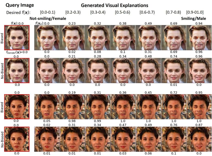
Under review as a conference paper at ICLR 2021

explanations that are limited to linear approximations of the ML model. Unfortunately, these linear
approximations are often inaccurate. In contrast, counterfactual methods suggest changes in the in-
put that would lead to a change in the corresponding output, providing information not only about
where the change should be but also what the change should be.
Counterfactual explanations should be actionable, i.e., a user should be able to act on it. An action-
able explanation would suggest feasible changes like removing sunglasses instead of unrealistic ones
like adding more eyes to the user’s face. Counterfactual explanations that are valid, proximal, and
sparse are more likely to be actionable [49, 38]. That is, a counterfactual explanation that changes
the outcome of the ML model (valid) by changing the minimal number of input features (sparse),
while remaining close to the input (proximal). Generating a set of diverse explanations increases the
likelihood of finding an actionable explanation [49, 38]. A set of counterfactuals is diverse if each
one proposes to change a different set of attributes. Intuitively, each of these explanations shed light
on a different action that user can take to change the ML model’s outcome.
Current counterfactual generation methods like xGEM [26] generates a single explanation that is far
from the input. Thus, it fails to be proximal, sparse, and diverse. Progressive Exaggeration (PE) [53]
provides higher-quality explanations more proximal than xGEM, but it still fails to provide a diverse
set of explanations. In addition, the image generator of PE is trained on the same data as the ML
model in order to detect biases thereby limiting their applicability. Moreover, like the previous
methods in the literature, these two methods tend to produce trivial explanations. For instance, an
explanation that suggests to increase the ‘smile’ attribute of a ‘smile’ classifier for an already-smiling
face is trivial and it does not explain why a misclassification occurred. In this work, we focus on
diverse valuable explanations (DiVE), that is, valid, proximal, sparse, and non-trivial.
We propose Diverse Valuable Explanations (DiVE), an explainability method that can interpret a
ML model by identifying sets of valuable attributes that have the most effect on the ML model’s
output. DiVE produces multiple counterfactual explanations which are enforced to be valuable,
and diverse resulting in more actionable explanations than the previous literature. Our method
first learns a generative model of the data using a β-TCVAE [5] to obtain a disentangled latent
representation which leads to more proximal and sparse explanations. In addition, the VAE is not
required to be trained on the same dataset as the ML model to be explained. DiVE then learns a latent
perturbation using constraints to enforce diversity, sparsity, and proximity. In order to generate non-
trivial explanations, DiVE leverages the Fisher information matrix of its latent space to focus its
search on the less influential factors of variation of the ML model. This mechanism enables the
discovery of spurious correlations learned by the ML model.
We provide experiments to assess whether our explanations are more valuable and diverse than
current state-of-the-art. First, we assess their validity on the CelebA dataset [33] and provide quan-
titative and qualitative results on a bias detection benchmark [53]. Second, we show that the gen-
erated explanations are more proximal in terms of Fréchet Inception Distance (FID) [19], which is
a measure of similarity between two datasets of images commonly used to evaluate the generation
quality of GAN. In addition, we evaluate the latent space closeness and face verification accuracy,
as reported by Singla et al. [53]. Third, we assess the sparsity of the generated counterfactuals by
computing the average change in facial attributes. Fourth, we show that DiVE is more successful
at finding more non-trivial explanations than previous methods and baselines. In the supplementary
material we provide additional results on the out-of-distribution performance of DiVE.
We summarize the contributions of this work as follows: 1) We propose DiVE, an explainability
method that can interpret a ML model by identifying the attributes that have the most effect on
its output. 2) DiVE achieves state of the art in terms of the validity, proximity, and sparsity of its
explanations, detecting biases on the datasets, and producing multiple explanations for an image. 3)
We identify the importance of finding non-trivial explanations and we propose a new benchmark
to evaluate how valuable the explanations are. 4) We propose to leverage the Fisher information
matrix of the latent space for finding spurious features that produce non-trivial explanations.

2    R ELATED W ORK

Explainable artificial intelligence (XAI) is a suite of techniques developed to make either the con-
struction or interpretation of model decisions more accessible and meaningful. Broadly speaking,
there are two branches of work in XAI, ad-hoc and post-hoc. Ad-hoc methods focus on making mod-

                                                    2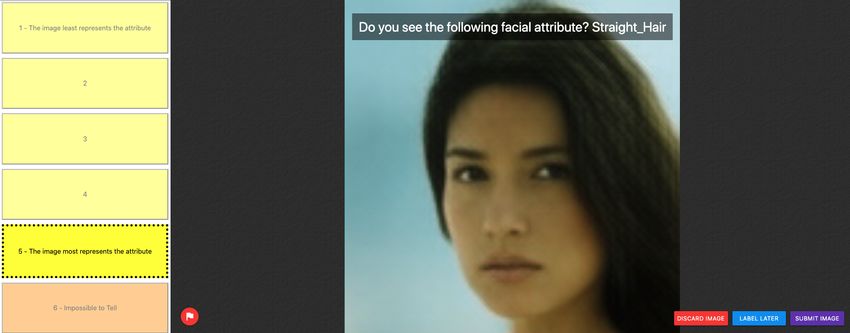
Under review as a conference paper at ICLR 2021

els interpretable, by imbuing model components or parameters with interpretations that are rooted
in the data themselves [45, 39, 25]. Unfortunately, most successful machine learning methods, in-
cluding deep learning ones, are uninterpretable [6, 32, 18, 24].
Post-hoc methods aim to explain the decisions of non interpretable models. These methods can
be categorized as non-generative and generative. Non-generative methods use information from a
ML model to identify the features most responsible for an outcome for a given input. Approaches
like [47, 37, 41] interpret ML model decisions by using derived information to fit a locally in-
terpretable model. Others use the gradient of the ML model parameters to perform feature attri-
bution [59, 60, 52, 54, 50, 1, 51], sometimes by employing a reference distribution for the fea-
tures [51, 11]. This has the advantage of identifying alternative feature values that when substituted
for the observed values would result in a different mode outcome. These methods are limited to
small contiguous regions of features with high influence on the target model outcome. In so doing,
they can struggle to provide plausible changes of the input that are actionable by an user in order to
correct a certain output or bias of the model. Generative methods such as [7, 5, 4] propose plausible
modifications of the input that change the model decision. However the generated perturbations
are usually found in pixel space and thus are bound to masking small regions of the image without
necessarily having a semantic meaning. Closest to our work are generative counterfactual expla-
nation methods [26, 9, 15, 53] which synthesize perturbed versions of observed data that result in
a corresponding change of the model prediction. While these methods provide valid and proximal
explanations for a model outcome, they fail to provide a diverse set of non-trivial explanations.
Mothilal et al. [38] addressed the diversity problem by introducing a diversity constraint between
a set of randomly initialized counterfactuals (DICE). However, DICE shares the same problems as
[7, 4] since perturbations are directly performed on the observed feature space, and does not take
into account trivial explanations.
In this work we propose DiVE, a counterfactual explanation method that generates a diverse set
of valid, proximal, sparse, and non-trivial explanations. Appendix A provides a more exhaustive
review of the related work.

3     P ROPOSED M ETHOD

We propose DiVE, an explainability method that can interpret a ML model by identifying the latent
attributes that have the most effect on its output. Summarized in Figure 1, DiVE uses an encoder,
a decoder, and a fixed weight ML model. The ML model could be any function for which we have
access to its gradients. In this work, we focus on a binary image classifier in order to produce visual
explanations. DiVE consists of two main steps. First, the encoder and the decoder are trained in
an unsupervised manner to approximate the data distribution on which the ML model was trained.
Unlike PE [53], our encoder-decoder model does not need to train on the same dataset that the ML
model was trained on. Second, we optimize a set of vectors i to perturb the latent representation z
generated by the trained encoder. The details of the optimization procedure are provided in Algo-
rithm 1 in the Appendix. We use the following 3 main losses for this optimization: a counterfactual
loss LCF that attempts to fool the ML model, an proximity loss Lprox that constrains the expla-
nations with respect to the number of changing attributes, and a diversity loss Ldiv that enforces
the explainer to generate diverse explanations with only one confounding factor for each of them.
Finally, we propose several strategies to mask subsets of dimensions in the latent space to prevent
the explainer from producing trivial explanations. Next we explain the methodology in more detail.

3.1   O BTAINING MEANINGFUL REPRESENTATIONS .

Given a data sample x ∈ X , its corresponding target y ∈ {0, 1}, and a potentially biased ML
model f (x) that approximates p(y|x), our method finds a perturbed version of the same input x̃ that
produces a desired probabilistic outcome ỹ ∈ [0, 1], so that f (x̃) = ỹ. In order to produce semanti-
cally meaningful counterfactual explanations, perturbations are performed on a latent representation
z ∈ Z ⊆ Rd of the input x. Ideally, each dimension in Z represents a different semantic concept of
the data, i.e., the different dimensions are disentangled.
For training the encoder-decoder architecture we use β-TCVAE [5] since it has been shown to obtain
competitive disentanglement performance [34]. It follows the same encoder-decoder structure as the

                                                  3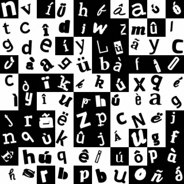
Under review as a conference paper at ICLR 2021

                                                                            Trivial Counterfactuals
      Z = Latent representation
        = Perturbation

                          Encoder                       Decoder             Not bald       Not bald
                                                                          Non-Trivial Counterfactuals

          Bald
                                                        ML model

                                                        Not Bald                Not bald   Not bald

Figure 1: DiVE encodes the input image (left) to explain into a latent representation z. Then z
is perturbed by  and decoded as counterfactual examples. During training, LCF finds the set of
 that change the ML model classifier outcome while Ldiv and Lprox enforce that the samples are
diverse while staying proximal. These are four valid counterfactuals generated from the experiment
in Section 4.4. However, only the bottom row contains counterfactuals where the man is still bald
as indicated by the oracle or a human. These counterfactuals identify a weakness in the ML model.

VAE [30], i.e., the input data is first encoded by a neural network qφ (z|x) parameterized by φ. Then,
the input data is recovered by a decoder neural network pθ (x|z), parameterized by θ. Using a prior
p(z) and a uniform distribution over the indexes of the dataset p(i), the original VAE loss is:
                 LV AE = Ep(i) Eq(z|xi ) [log pθ (xi |z)] − Ep(i) DKL (qφ (z|xi )||p(z)) ,              (1)
where the first term is the reconstruction loss and the second is the average divergence from the
prior. The core difference of β-TCVAE is the decomposition of this average divergence:
                                                                      P
       Ep(i) DKL qφ (z|xi )||p(z) → DKL (qφ (z, xi )||qφ (z)pθ (xi )) + j DKL (qφ (zj )||p(zj ))
                                                         Q
                                     + β · DKL qφ (z)|| j qφ (zj ) ,                             (2)
where the arrow represents a modification of the left terms and equality is obtained when β = 1.
The third term on the right hand side is called total correlation and measures the shared information
between all empirical marginals qφ (zj ) = Ep(i) qφ (zj |xi ). By using β > 1, this part is amplified and
encourages further decorrelations between the latent variables and leads to better disentanglement.
In addition to β-TCVAE, we use the perceptual reconstruction loss from Hou et al. [20]. This
replaces the pixel-wise reconstruction loss in Equation 1 by a perceptual reconstruction loss, using
the hidden representation of a pre-trained neural network R. Specifically, we learn a decoder Dθ
generating an image i.e., x̃ = Dθ (z), and this image is re-encoded in a hidden representation:
h = R(x̃), and compared to the original image in the same space using a normal distribution. The
reconstruction loss of Equation 1 now becomes:
                              Ep(i) Eq(z|xi ) [log N (R(xi ); R(Dθ (z)), I)],                           (3)
Once trained, the weights of the encoder-decoder are fixed for the rest of the steps of our algorithm.

3.2   I NTERPRETING THE ML MODEL

In order to find weaknesses in the ML model, DiVE searches for a collection of n latent perturbation
{i }ni=1 such that the decoded output x̃i = Dθ (z+i ) yields a specific response from the ML model,
i.e., f (x̃) = ỹ for any chosen ỹ ∈ [0, 1]. We optimize i ’s by minimizing:
         LDiVE (x, ỹ, {i }ni=1 ) = i LCF (x, ỹ, i ) + λ · i Lprox (x, i ) + α · Ldiv ({i }ni=1 ), (4)
                                    P                        P

where λ, and α determine the relative importance of the losses. The minimization is performed with
gradient descent and the complete algorithm can be found in Algorithm 1 in Appendix D. We now
describe the different loss terms.
Counterfactual loss. The goal of this loss function is to identify a change of latent attributes that
will cause the ML model f to change it’s prediction. For example, in face recognition, if the classifier

                                                    4
Under review as a conference paper at ICLR 2021
detects that there is a smile present whenever the hair is brown, then this loss function is likely to
change the hair color attribute. This is achieved by sampling from the decoder x̃ = Dθ (z + ), and
optimizing the binary cross-entropy between the target ỹ and the prediction f (x̃):
LCF (x, ỹ, ) = ỹ · log(f (x̃)) + (1 − ỹ) · log(1 − f (x̃)). (5)
Proximity loss. The goal of this loss function is to constrain the reconstruction produced by the
decoder to be similar in appearance and attributes as the input. It consists of the following two terms,
Lprox (x, ) = ||x − x̃||1 + γ · ||||1 , (6)
where γ is a scalar weighting the relative importance of the two terms. The first term ensures that
the explanations can be related to the input by constraining the input and the output to be similar.
The second term aims to identify a sparse perturbation to the latent space Z that confounds the
ML model. This constrains the explainer to identify the least amount of attributes that affect the
classifier’s decision in order to produce sparse explanations.
Diversity loss. This loss prevents the multiple explanations of the model from being identical. For
instance, if gender and hair color are spuriously correlated with smile, the model should provide
images either with different gender or different hair color. To achieve this, we jointly optimize for a
collection of n perturbations {i }ni=1 and minimize their pairwise similarity:
v
uX T 2
i j
Ldiv ({i }ni=1 ) = t
u
. (7)
ki k2 kj k2
i6=j
The method resulting of optimizing Eq. 4 (DiVE) results in diverse counterfactuals that are more
valid, proximal, and sparse. However, it may still produce trivial explanations, such as exaggerating
a smile to explain a smile classifier without considering other valuable biases in the ML model such
as hair color. While the diversity loss encourages the orthogonality of the explanations, there might
still be several latent variables required to represent all variations of smile.
Beyond trivial counterfactual explanations. To find non-trivial explanations, we propose to pre-
vent DiVE from perturbing the most influential latent factors of Z on the ML model. We estimate
the influence of each of the latent factors with the average Fisher information matrix:
F = Ep(i) Eqφ (z|xi ) Ep(y|z) ∇z ln p(y|z) ∇z ln p(y|z)T , (8)
where p(y = 1|z) = f (Dθ (z)), and p(y = 0|z) = 1 − f (Dθ (z)). The diagonal values of F express
the relative influence of each of the latent dimensions on the classifier output. Since the most influ-
ential dimensions are likely to be related to the main attribute used by the classifier, we propose to
prevent Eq. 4 from perturbing them in order to find more surprising explanations. Thus when pro-
ducing n explanations, we sort Z by the magnitude of the diagonal, we partition it into n contiguous
chunks that will be optimized for each of the explanations. We call this method DiVEFisher .
However, DiVEF isher does not guarantee that the different partitions of Z all the factors concerning
a trivial attribute are grouped together. Thus, we propose to partition Z into subsets of latent factors
that interact with each other when changing the predictions of the ML model. Such interaction can
be estimated using F as an affinity measure. We use spectral clustering [55] to obtain a partition of
Z. This partition is represented as a collection of mask {mi }ni=1 , where mi ∈ {0, 1}d represents
which dimensions of Z are part of cluster i. Finally, these masks are used in Equation 4 to bound
each i to its subspace i.e., 0i = i ◦ mi , where ◦ represents element wise multiplication. Since
these masks are orthogonal, this effectively replaces Ldiv . In Section 4, we highlight the benefits of
this clustering approach by comparing to other baselines. We call this method DiVEFisherSpectral .
4 E XPERIMENTAL R ESULTS
In this section, we evaluate the described methods on 5 different aspects: (1) the validity of the
generated explanations as well as the ability to discover biases within the ML model and the data
(Section 4.1); (2) their proximity in terms of FID, latent space closeness, and face verification accu-
racy (Section 4.2); (3) the sparsity of the generated counterfactuals (Section 4.3); and (4) the ability
to identify diverse non-trivial explanations for image misclassifications made by the ML model
(Section 4.4); (5) the out-of-distribution performance of DiVE (Section 4.4).
5Under review as a conference paper at ICLR 2021
Table 1: Bias detection experiment. Ratio of
generated counterfactuals classified as “Smiling” Table 2: FID of DiVE compared to xGEM [26],
and “Non-Smiling” for a classifier biased on gen- Progressive Exaggeration (PE) [53], xGEM
der (fbiased ) and an unbiased classifier (funbiased ). trained with our backbone (xGEM+), and DiVE
Bold indicates Overall closest to the Ground truth. trained without the perceptual loss (DiVE--)
Target label Target Attribute xGEM PE xGEM+ DiVE-- DiVE
ML model Smiling Non-Smiling Smiling
model PE xGEM+ DiVE PE xGEM+ DiVE
Male 0.52 0.94 0.89 0.18 0.24 0.16
Present 111.0 46.9 67.2 54.9 30.6
fbiased Female 0.48 0.06 0.11 0.82 0.77 0.84 Absent 112.9 56.3 77.8 62.3 33.6
Overall 0.12 0.29 0.22 0.35 0.33 0.36 Overall 106.3 35.8 66.9 55.9 29.4
Ground truth 0.75 0.67
Young
Male 0.48 0.41 0.42 0.47 0.38 0.44
funbiased Female 0.52 0.59 0.58 0.53 0.62 0.57 Present 115.2 67.6 68.3 57.2 31.8
Overall 0.07 0.13 0.10 0.08 0.15 0.07 Absent 170.3 74.4 76.1 51.1 45.7
Ground truth 0.04 0.00 Overall 117.9 53.4 59.5 47.7 33.8
Experimental Setup. As common procedure [26, 9, 53], we perform experiments on the CelebA
database [33]. CelebA is a large-scale dataset containing more than 200K celebrity facial images.
Each image is annotated with 40 binary attributes such as “Smiling”, “Male”, and “Eyeglasses”.
These attributes allow us to evaluate counterfactual explanations by determining whether they could
highlight spurious correlations between multiple attributes such as “lipstick” and “smile”. In this
setup, explainability methods are trained in the training set and ML models are explained on the
validation set. The hyperparameters of the explainer are searched by cross-validation on the training
set. We use the same train and validaton splits as PE [53]. Explainers do not have access to the
labeled attributes during training.
We test the out-of-distribution (OOD) performance of DiVE with the Synbols dataset [31]. Synbols
is an image generator with characters from the Unicode standard and the wide range of artistic fonts
provided by the open font community. This provides us to better control on the features present in
each set when compared to CelebA. We generate 100K black and white of 32×32 images from 48
characters in the latin alphabet and more than 1K fonts. We use the character type to create disjoint
sets for OOD training and we use the fonts to introduce biases in the data. We provide a sample of
the dataset in Figure 8 in Appendix I.
We compare four versions of our method to three existing methods. DiVE, resulting of optimizing
Eq. 4. DiVEFisher , which extends DiVE by using the Fisher information matrix introduced in Eq. 8.
DiVEFisherSpectral , which extends DiVEFisher with spectral clustering. We introduce two additional
ablations of our method, DiVE-- and DiVERandom . DiVE-- is equivalent to DiVE but using a pixel-
based reconstruction loss instead of the perceptual loss. DiVERandom uses random masks instead of
using the Fisher information. Finally, we compare our baselines with xGEM as described in Joshi
et al. [26], xGEM+, which is the same as xGem but uses the same auto-encoding architecture as
DiVE, and PE as described by Singla et al. [53]. For our methods, we provide implementation
details, architecture description, and algorithm in Appendix D.
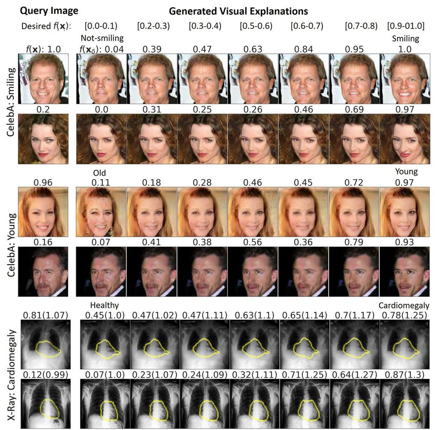
4.1 VALIDITY AND BIAS DETECTION
We evaluate DiVE’s ability to detect biases in the data. We follow the same procedure as PE [53],
and train two binary classifiers for the attribute “Smiling”. The first one is trained on a biased version
of CelebA where all the male celebrities are smiling and all the female are not smiling (fbiased ). The
second one is trained on the unbiased version of the data (funbiased ). Both classifiers are evaluated
on the CelebA validation set. Also following Singla et al. [53], we train an oracle classifier (foracle )
based on VGGFace2 [3] which obtains perfect accuracy on the gender attribute. The hypothesis
is that if “Smiling” and gender are confounded by the classifier, so should be the explanations.
Therefore, we could identify biases when the generated examples not only change the target attribute
but also the confounded one. To generate the counterfactuals, DiVE produces perturbations until it
changes the original prediction of the classifier (e.g. “Smiling” to “Non-Smiling”).
We follow the procedure introduced in [26, 53] and report a confounding metric for bias detection
in In Table 1. The columns Smiling and Non-Smiling indicate the target class for counterfactual
generation. The rows Male and Female contain the proportion of counterfactuals that are classified
by the oracle as Male and Female. We can see that the generated explanations for fbiased are classified
6Under review as a conference paper at ICLR 2021
Table 3: Average number attributes changed per explanation and percentage of non-trivial explana-
tions. This experiment evaluates the counterfactuals generated by different methods for a ML model
trained on the attribute ‘Young’ of the CelebA dataset. xGEM++ is xGEM+ using β-TCVAE as
generator.
PE [53] xGEM+ [26] xGEM++ DiVE DiVEFisher DiVEFisherSpectral
Attr. change 03.74 06.92 06.70 04.81 04.82 04.58
Non-trivial (%) 05.12 18.56 34.62 43.51 42.99 51.07
more often as Male when the target attribute is Smiling and Female when the target attribute is Non-
Smiling. The confounding metric, denoted as overall, is the fraction of generated explanations for
which the gender was changed with respect to the original image. It thus reflect the magnitude of
the the bias as approximated by the explainers.
Singla et al. [53] consider that a model is better than another if the confounding metric is the highest
on fbiased and the lowest on funbiased . However, they assume that fbiased always predicts the Gender
based on Smile. Instead, we propose to evaluate the confounding metric by comparing it to the
empirical bias of the model, denoted as ground truth in the Table 1. Details provided in Appendix J.
We observe that DiVE is more successful than PE at detecting biases although the generative model
of DiVE was not trained with the biased data. While xGEM+ has a higher success rate at detecting
biases in some cases, it produces lower-quality images that are far from the input. In Figure 5 in
Appendix B, we provide samples generated by our method with the two classifiers and compare
them to PE and xGEM+. We found that gender changes with the “Smiling” attribute with fbiased
while for funbiased it stayed the same. In addition, we also observed that for fbiased the correlation
between “Smile” and “Gender” is higher than for PE. It can also be observed that xGEM+ fails to
retain the identity of the person in x when compared to PE and our method.
4.2 C OUNTERFACTUAL E XPLANATION P ROXIMITY
We evaluate the proximity of the counterfactual explanations using FID scores [19] as described
by Singla et al. [53]. The scores are based on the target attributes “Smiling” and “Young”, and
are divided into 3 categories: Present, Absent, and Overall. Present considers explanations for
which the ML model outputs a probability greater than 0.9 for the target attribute. Absent refers to
explanations with a probability lower than 0.1. Overall considers all the successful counterfactuals,
which changed the original prediction of the ML model.
We report these scores in Table 2 for all 3 categories. DiVE produces the best quality counterfactuals,
surpassing PE by 6.3 FID points for the “Smiling” target and 19.6 FID points for the “Young” target
in the Overall category. DiVE obtains lower FID than xGEM+ which shows that the improvement
not only comes from the superior architecture of our method. Further, there are two other factors that
explain the improvement of DiVE’s FID. First, the β-TCVAE decomposition of the KL divergence
improves the disentanglement ability of the model while suffering less reconstruction degradation
than the VAE. Second, the perceptual loss makes the image quality constructed by DiVE to be
comparable with that of the GAN used in PE. In addition, Table 4 in the Appendix shows that DiVE
is more successful at preserving the identity of the faces than PE and xGEM and thus at producing
feasible explanations. These results suggest that the combination of disentangled latent features and
the regularization of the latent features help DiVE to produce the minimal perturbations of the input
that produce a successful counterfactual.
In Figure 5 in Appendix B we show qualitative results obtained by targeting different probability
ranges for the output of the ML model as described in PE. As seen in Figure 5, DiVE produces
more natural-looking facial expressions than xGEM+ and PE. Additional results for “Smiling” and
“Young” are provided in Figures 3 and 4 in the Appendix B.
4.3 C OUNTERFACTUAL E XPLANATION S PARSITY
Explanations that produce sparse changes in the attributes of the image are more probable to be
actionable. In this section we quantitatively compare the amount of valid and sparse counterfactuals
provided by different baselines. Table 3 shows the results for a classifier model trained on the at-
7Under review as a conference paper at ICLR 2021
tribute Young of the CelebA dataset.1 The first row shows the number of attributes that each method
change in average to generate a valid counterfactual. Methods that require to change less attributes
are likely to be more actionable. We observe that DiVE changes less attributes on average than
xGEM+. We also observe that DiVEFisherSpectral is the method that changes less attributes among all
the baselines. To better understand the effect of disentangled representations, we also report results
for a version of xGEM+ with the β-TCVAE backbone (xGEM++). We do not observe significant
effects on the sparsity of the counterfactuals. In fact, a fine-grained decomposition of concepts in
the latent space could lead to lower the sparsity.
4.4 B EYOND TRIVIAL EXPLANATIONS
Previous works on counterfactual generations tend to produce trivial input perturbations to change
the output of the ML model. That is, they tend to increase/decrease the presence of the attribute that
the classifier is predicting. For instance, in Figure 5 all the explainers put a smile on the input face in
order to increase the probability for “smile”. While that is correct, this explanation does not provide
much insight about the potential weaknesses of the ML model. Instead, in this work we emphasize
producing non-trivial explanations, that are different from the main attribute that the ML model has
been trained to identify. These kind of explanations provide more insight about the factors that affect
the classifier and thus provide cues on how to improve the model or how to fix incorrect predictions.
To evaluate this, we propose a new benchmark that measures a method’s ability to generate valuable
explanations. For an explanation to be valuable, it should 1) be misclassified by the ML model
(valid), 2) not modify the main attribute being classified (non-trivial), and 3) not have diverged too
much from the original sample (proximal). A misclassification provides insights into the weaknesses
of the model. However, the counterfactual is even more insightful when it stays close to the original
image as it singles-out spurious correlations learned by the ML model. Because it is costly to provide
human evaluation of an automatic benchmark, we approximate both the proximity and the real class
with the VGGFace2-based oracle. We choose the VGGFace2 model as it is less likely to share the
same biases as the ML model, since it was trained for a different task than the ML model with an
order of magnitude more data. We conduct a human evaluation experiment in Appendix F, and we
find a significant correlation between the oracle and the human predictions. For 1) and 2) we deem
that an explanation is successful if the ML model and the oracle make different predictions about
the counterfactual. E.g., the top counterfactuals in Figure 1 are not deemed successful explanations
because both the ML model and the oracle agree on its class, however the two in the bottom row are
successful because only the oracle made the correct prediction. These explanations where generated
by DiVEFisherSpectral . As for 3) we measure the proximity with the cosine distance between the sample
and the counterfactual in the feature space of the oracle.
We test all methods from Section 4 on a subset of the CelebA validation set described in Appendix E.
We report the results of the full hyperparameter search (see Appendix E) in Figure 2a. The vertical
axis shows the success rate of the explainers, i.e., the ratio of valid explanations that are non-trivial.
This is the misclassification rate of the ML model on the explanations. The dots denote the mean
performances and the curves are computed with Kernel Density Estimation (KDE). On average,
DiVE improves the similarity metric over xGEM+ highlighting the importance of disentangled rep-
resentations for identity preservation. Moreover, using information from the diagonal of the Fisher
Information Matrix as described in Eq. 8 further improves the explanations as shown by the higher
success rate of DiVEFisher over DiVE and DiVERandom . Thus, preventing the model from perturbing
the most influential latent factors helps to uncover spurious correlations that affect the ML model.
Finally, the proposed spectral clustering of the full Fisher Matrix attains the best performance vali-
dating that the latent space partition can guide the gradient-based search towards better explanations.
We reach the same conclusions in Table 3, where we provide a comparison with PE for the attribute
Young. In addition, we provide results for a version of xGEM+ with more disentangled latent factos
(xGEM++). We find that disentangled representations provide the explainer with a more precise
control on the semantic concepts being perturbed, which increases the success rate of the explainer
by 16%.
Out-of-distribution generalization. In the previous experiments, the generative model of DiVE
was trained on the same data distribution (i.e., CelebA faces) as the ML model. We test the out-
1
The code and pre-trained models of PE are only available for the attribute Young.
8Under review as a conference paper at ICLR 2021
0.7
xGEM+ 0.70 xGEM+ xGEM+
DiVE DiVERandom 0.8 DiVERandom
0.6
random 0.65 DiVE DiVE
0.5 DiVE_Fisher DiVEFisher 0.7 DiVEFisher
DiVE_FisherSpectral 0.60 DiVEFisherSpectral DiVEFisherSpectral
0.4
0.6
success rate
success rate
success rate
0.55
0.3
0.2 0.50 0.5
0.1 0.45
0.4
0.0 0.40
0.1 0.3
0.35
0.75 0.80 0.85 0.90 0.95 0.5 0.6 0.7 0.8 0.9 1.0 0.65 0.70 0.75 0.80 0.85 0.90
embedding similarity (VGG) embedding similarity (Resnet12) embedding similarity (Resnet12)
(a) CelebA (ID) (b) Synbols (ID) (c) Synbols (OOD)
Figure 2: Beyond trivial explanations. The rate of successful explanations (y-axis) plotted against
embedding similarity (x-axis) for all methods. For both metrics, higher is better, i.e., the most valu-
able explanations are in the top-right corner. For each method, we ran an hyperparameter sweep
and denote the mean of the performances with a dot. The curves are computed with KDE. The
left plot shows the performance on CelebA and the other two plots shows the performance for in-
distribution (ID) and out-of-distribution (OOD) experiments on Synbols . All DiVE methods outper-
form xGEM+ on both metrics simultaneously when conditioning on successful counterfactuals. In
both experiments, DiVEFisher and DiVEFisherSpectral improve the performance over both DiVERandom
and DiVE.
.
of-distribution performance of DiVE by training its auto-encoder on a subset of the latin alphabet
of the Synbols dataset [31]. Then, counterfactual explanations are produced for a different disjoint
subset of the alphabet. To evaluate the effectiveness of DiVE in finding biases on the ML model,
we introduce spurious correlations in the data. Concretely, we assign different fonts to each of
the letters in the alphabet as detailed in Appendix I. In-distribution (ID) results are reported in
Figure 2b for reference, and OD results are reported in Figure 2c. We observe that DiVE is able
to find valuable countefactuals even when the VAE was not trained on the same data distribution.
Moreover, results are consistent with the CelebA experiment, with DiVE outperforming xGEM+
and Fiser information-based methods outperforming the rest.
5 L IMITATIONS AND F UTURE W ORK
This work shows that a good generative model can provide interesting insights on the biases of a ML
model. However, this relies on a properly disentangled representation. In the case where the gener-
ative model would be heavily entangled it would fail to produce explanations with a sparse amount
of features. However, our approach can still tolerate a small amount of entanglement, yielding a
small decrease in interpretability. We expect that progress in identifiability [35, 28] will increase the
quality of representations. With a perfectly disentangled model, our approach could still miss some
explanations or biases. E.g., with the spectral clustering of the Fisher, we group latent variables and
only produce a single explanation per group in order to present explanations that are conceptually
different. This may leave behind some important explanations, but the user can simply increase the
number of clusters or the number of explanation per clusters for a more in-depth analysis.
In addition to the challenge of achieving disentangled representations, finding the optimal hyperpa-
rameters for the VAE and their generalization out of the training distribution is an open problem.
Moreover, if the generative model is trained on biased data, one could expect the counterfactuals to
be biased as well. However, as we show in Figure 2c, our model still finds non-trivial explanations
when applied out of distribution. In that way, it could be trained on a larger unlabeled dataset to
overcome possible biases caused by the lack of annotated data.
Although the generative model plays an important role to produce actionable counterfactuals in the
computer vision domain domain, our work could be extended to other domains. For example, Eq. 4
could be applied to find non-trivial explanations on tabular data by directly optimizing the observed
features instead of the latent factors of the VAE. However, further work would be needed to adapt
the DiVE loss functions to produce perturbations on discrete and categorical variables.
9Under review as a conference paper at ICLR 2021
R EFERENCES
[1] Julius Adebayo, Justin Gilmer, Michael Muelly, Ian Goodfellow, Moritz Hardt, and Been Kim.
Sanity checks for saliency maps. In Advances in Neural Information Processing Systems, 2018.
[2] Andrew Brock, Jeff Donahue, and Karen Simonyan. Large scale gan training for high fidelity
natural image synthesis. arXiv preprint arXiv:1809.11096, 2018.
[3] Q. Cao, L. Shen, W. Xie, O. M. Parkhi, and A. Zisserman. Vggface2: A dataset for recog-
nising faces across pose and age. In International Conference on Automatic Face and Gesture
Recognition, 2018.
[4] Chun-Hao Chang, Elliot Creager, Anna Goldenberg, and David Duvenaud. Explaining image
classifiers by counterfactual generation. In International Conference on Learning Representa-
tions, 2019.
[5] Ricky TQ Chen, Xuechen Li, Roger B Grosse, and David K Duvenaud. Isolating sources of
disentanglement in variational autoencoders. In Advances in Neural Information Processing
Systems, 2018.
[6] Corinna Cortes and Vladimir Vapnik. Support-vector networks. Machine learning, 20(3):
273–297, 1995.
[7] Piotr Dabkowski and Yarin Gal. Real time image saliency for black box classifiers. arXiv
preprint arXiv:1705.07857, 2017.
[8] Jia Deng, Wei Dong, Richard Socher, Li-Jia Li, Kai Li, and Li Fei-Fei. Imagenet: A large-scale
hierarchical image database. In Computer Vision and Pattern Recognition, 2009.
[9] Emily Denton, Ben Hutchinson, Margaret Mitchell, and Timnit Gebru. Detecting bias with
generative counterfactual face attribute augmentation. arXiv preprint arXiv:1906.06439, 2019.
[10] Amit Dhurandhar, Pin-Yu Chen, Ronny Luss, Chun-Chen Tu, Paishun Ting, Karthikeyan Shan-
mugam, and Payel Das. Explanations based on the missing: Towards contrastive explanations
with pertinent negatives. In Advances in Neural Information Processing Systems, pp. 592–603,
2018.
[11] Ruth C Fong and Andrea Vedaldi. Interpretable explanations of black boxes by meaningful
perturbation. In International Conference on Computer Vision, 2017.
[12] Hao Fu, Chunyuan Li, Xiaodong Liu, Jianfeng Gao, Asli Celikyilmaz, and Lawrence Carin.
Cyclical annealing schedule: A simple approach to mitigating kl vanishing. arXiv preprint
arXiv:1903.10145, 2019.
[13] Yarin Gal, Jiri Hron, and Alex Kendall. Concrete dropout. In Advances in neural information
processing systems, 2017.
[14] Ian Goodfellow, Jean Pouget-Abadie, Mehdi Mirza, Bing Xu, David Warde-Farley, Sherjil
Ozair, Aaron Courville, and Yoshua Bengio. Generative adversarial nets. In Advances in
Neural Information Processing Systems, 2014.
[15] Yash Goyal, Ziyan Wu, Jan Ernst, Dhruv Batra, Devi Parikh, and Stefan Lee. Counterfactual
visual explanations. arXiv preprint arXiv:1904.07451, 2019.
[16] Riccardo Guidotti, Anna Monreale, Fosca Giannotti, Dino Pedreschi, Salvatore Ruggieri, and
Franco Turini. Factual and counterfactual explanations for black box decision making. IEEE
Intelligent Systems, 34(6):14–23, 2019.
[17] Riccardo Guidotti, Anna Monreale, Stan Matwin, and Dino Pedreschi. Black box explanation
by learning image exemplars in the latent feature space. In Joint European Conference on
Machine Learning and Knowledge Discovery in Databases, pp. 189–205. Springer, 2019.
[18] Kaiming He, Xiangyu Zhang, Shaoqing Ren, and Jian Sun. Deep residual learning for image
recognition. In Computer Vision and Pattern Recognition, 2016.
10Under review as a conference paper at ICLR 2021
[19] Martin Heusel, Hubert Ramsauer, Thomas Unterthiner, Bernhard Nessler, and Sepp Hochreiter.
Gans trained by a two time-scale update rule converge to a local nash equilibrium. In Advances
in Neural Information Processing Systems, 2017.
[20] Xianxu Hou, Linlin Shen, Ke Sun, and Guoping Qiu. Deep feature consistent variational
autoencoder. In Winter Conference on Applications of Computer Vision, 2017.
[21] Gao Huang, Zhuang Liu, Laurens Van Der Maaten, and Kilian Q Weinberger. Densely con-
nected convolutional networks. In Computer Vision and Pattern recognition, 2017.
[22] Farhad Imani, Ruimin Chen, Evan Diewald, Edward Reutzel, and Hui Yang. Deep learning
of variant geometry in layerwise imaging profiles for additive manufacturing quality control.
Journal of Manufacturing Science and Engineering, 141(11), 2019.
[23] Sergey Ioffe and Christian Szegedy. Batch normalization: Accelerating deep network training
by reducing internal covariate shift. In International Conference on Machine Learning, 2015.
[24] Simon Jégou, Michal Drozdzal, David Vazquez, Adriana Romero, and Yoshua Bengio. The
one hundred layers tiramisu: Fully convolutional densenets for semantic segmentation. In
Computer Vision and Pattern Recognition Workshops, 2017.
[25] Finn V Jensen et al. An introduction to Bayesian networks, volume 210. UCL press London,
1996.
[26] Shalmali Joshi, Oluwasanmi Koyejo, Been Kim, and Joydeep Ghosh. xgems: Generating
examplars to explain black-box models. arXiv preprint arXiv:1806.08867, 2018.
[27] Amir-Hossein Karimi, Gilles Barthe, Borja Balle, and Isabel Valera. Model-agnostic coun-
terfactual explanations for consequential decisions. In International Conference on Artificial
Intelligence and Statistics, pp. 895–905, 2020.
[28] Ilyes Khemakhem, Diederik Kingma, Ricardo Monti, and Aapo Hyvarinen. Variational au-
toencoders and nonlinear ica: A unifying framework. In International Conference on Artificial
Intelligence and Statistics, pp. 2207–2217. PMLR, 2020.
[29] Diederik P Kingma and Jimmy Ba. Adam: A method for stochastic optimization. arXiv
preprint arXiv:1412.6980, 2014.
[30] Diederik P Kingma and Max Welling. Auto-encoding variational bayes. arXiv preprint
arXiv:1312.6114, 2013.
[31] Alexandre Lacoste, Pau Rodrı́guez López, Frédéric Branchaud-Charron, Parmida Atighe-
hchian, Massimo Caccia, Issam Hadj Laradji, Alexandre Drouin, Matthew Craddock, Laurent
Charlin, and David Vázquez. Synbols: Probing learning algorithms with synthetic datasets.
Advances in Neural Information Processing Systems, 33, 2020.
[32] Yann LeCun, Bernhard Boser, John S Denker, Donnie Henderson, Richard E Howard, Wayne
Hubbard, and Lawrence D Jackel. Backpropagation applied to handwritten zip code recogni-
tion. Neural Computation, 1(4):541–551, 1989.
[33] Ziwei Liu, Ping Luo, Xiaogang Wang, and Xiaoou Tang. Deep learning face attributes in the
wild. In International Conference on Computer Vision, 2015.
[34] Francesco Locatello, Stefan Bauer, Mario Lucic, Gunnar Raetsch, Sylvain Gelly, Bernhard
Schölkopf, and Olivier Bachem. Challenging common assumptions in the unsupervised learn-
ing of disentangled representations. In International Conference on Machine Learning, 2019.
[35] Francesco Locatello, Ben Poole, Gunnar Rätsch, Bernhard Schölkopf, Olivier Bachem, and
Michael Tschannen. Weakly-supervised disentanglement without compromises. arXiv preprint
arXiv:2002.02886, 2020.
[36] James Lucas, George Tucker, Roger Grosse, and Mohammad Norouzi. Understanding poste-
rior collapse in generative latent variable models. 2019.
11Under review as a conference paper at ICLR 2021
[37] Scott M Lundberg and Su-In Lee. A unified approach to interpreting model predictions. In
Advances in neural information processing systems, 2017.
[38] Ramaravind K Mothilal, Amit Sharma, and Chenhao Tan. Explaining machine learning classi-
fiers through diverse counterfactual explanations. In Conference on Fairness, Accountability,
and Transparency, 2020.
[39] John Ashworth Nelder and Robert WM Wedderburn. Generalized linear models. Journal of
the Royal Statistical Society: Series A (General), 135(3):370–384, 1972.
[40] Boris Oreshkin, Pau Rodrı́guez López, and Alexandre Lacoste. Tadam: Task dependent adap-
tive metric for improved few-shot learning. Advances in Neural Information Processing Sys-
tems, 31:721–731, 2018.
[41] Nicolas Papernot and Patrick McDaniel. Deep k-nearest neighbors: Towards confident, inter-
pretable and robust deep learning. arXiv preprint arXiv:1803.04765, 2018.
[42] Martin Pawelczyk, Klaus Broelemann, and Gjergji Kasneci. Learning model-agnostic coun-
terfactual explanations for tabular data. In Proceedings of The Web Conference 2020, pp.
3126–3132, 2020.
[43] Ethan Perez, Florian Strub, Harm De Vries, Vincent Dumoulin, and Aaron Courville. Film:
Visual reasoning with a general conditioning layer. arXiv preprint arXiv:1709.07871, 2017.
[44] Rafael Poyiadzi, Kacper Sokol, Raul Santos-Rodriguez, Tijl De Bie, and Peter Flach. Face:
feasible and actionable counterfactual explanations. In Proceedings of the AAAI/ACM Confer-
ence on AI, Ethics, and Society, pp. 344–350, 2020.
[45] J. R. Quinlan. Induction of decision trees. Machine Learning, 1:81–106, 1986.
[46] Prajit Ramachandran, Barret Zoph, and Quoc V Le. Searching for activation functions. Inter-
national Conference on Learning Representations, 2018.
[47] Marco Tulio Ribeiro, Sameer Singh, and Carlos Guestrin. ”why should i trust you?” explaining
the predictions of any classifier. In International Conference on Knowledge Discovery and
Data Mining, 2016.
[48] German Ros, Sebastian Ramos, Manuel Granados, Amir Bakhtiary, David Vazquez, and An-
tonio M Lopez. Vision-based offline-online perception paradigm for autonomous driving. In
Winter Conference on Applications of Computer Vision, 2015.
[49] Chris Russell. Efficient search for diverse coherent explanations. In Conference on Fairness,
Accountability, and Transparency, 2019.
[50] Ramprasaath R Selvaraju, Michael Cogswell, Abhishek Das, Ramakrishna Vedantam, Devi
Parikh, and Dhruv Batra. Grad-cam: Visual explanations from deep networks via gradient-
based localization. In International Conference on Computer Vision, 2017.
[51] Avanti Shrikumar, Peyton Greenside, and Anshul Kundaje. Learning important features
through propagating activation differences. arXiv preprint arXiv:1704.02685, 2017.
[52] Karen Simonyan, Andrea Vedaldi, and Andrew Zisserman. Deep inside convolutional
networks: Visualising image classification models and saliency maps. arXiv preprint
arXiv:1312.6034, 2013.
[53] Sumedha Singla, Brian Pollack, Junxiang Chen, and Kayhan Batmanghelich. Explanation by
progressive exaggeration. In International Conference on Learning Representations, 2020.
[54] Jost Tobias Springenberg, Alexey Dosovitskiy, Thomas Brox, and Martin Riedmiller. Striving
for simplicity: The all convolutional net. arXiv preprint arXiv:1412.6806, 2014.
[55] X Yu Stella and Jianbo Shi. Multiclass spectral clustering. In null, pp. 313. IEEE, 2003.
[56] Dmitry Ulyanov, Andrea Vedaldi, and Victor Lempitsky. Instance normalization: The missing
ingredient for fast stylization. arXiv preprint arXiv:1607.08022, 2016.
12Under review as a conference paper at ICLR 2021
[57] Arnaud Van Looveren and Janis Klaise. Interpretable counterfactual explanations guided by
prototypes. arXiv preprint arXiv:1907.02584, 2019.
[58] David Vázquez, Jorge Bernal, F Javier Sánchez, Gloria Fernández-Esparrach, Antonio M
López, Adriana Romero, Michal Drozdzal, and Aaron Courville. A benchmark for endolu-
minal scene segmentation of colonoscopy images. Journal of healthcare engineering, 2017.
[59] Bolei Zhou, Aditya Khosla, Agata Lapedriza, Aude Oliva, and Antonio Torralba. Object de-
tectors emerge in deep scene cnns. arXiv preprint arXiv:1412.6856, 2014.
[60] Bolei Zhou, Aditya Khosla, Agata Lapedriza, Aude Oliva, and Antonio Torralba. Learning
deep features for discriminative localization. In Computer Vision and Pattern Recognition,
2016.
13Under review as a conference paper at ICLR 2021
A PPENDIX
A E XTENDED R ELATED W ORK
Counterfactual explanation lies inside a more broadly-connected body of work for explaining clas-
sifier decisions. Different lines of work share this goal but vary in the assumptions they make about
what elements of the model and data to emphasize as way of explanation.
Model-agnostic counterfactual explanation. Like [47, 37], these models make no assumptions
about model structure, and interact solely with its label predictions. Karimi et al. [27] develop a
model agnostic, as well as metric agnostic approach. They reduce the search for counterfactual ex-
planations (along with user-provided constraints) into a series of satisfiability problems to be solved
with off-the-shelf SAT solvers. Similar in spirit to [47], Guidotti et al. [16] first construct a local
neighbourhood around test instances, finding both positive and negative exemplars within the neigh-
bourhood. These are used to learn a shallow decision tree, and explanations are provided in terms
of the inspection of its nodes and structure. Subsequent work builds on this local neighbourhood
idea [17], but specializes to medical diagnostic images. They use a VAE to generate both positive
and negative samples, then use random heuristic search to arrive at a balanced set. The generated
explanatory samples are used to produce a saliency feature map for the test data point by considering
the median absolute deviation of pixel-wise differences between the test point, and the positive and
negative example sets.
Gradient based feature attribution. These methods identify input features responsible for the
greatest change in the loss function, as measured by the magnitude of the gradient with respect to
the inputs. Early work in this area focused on how methodological improvements for object detec-
tion in images could be re-purposed for feature attribution [59, 60], followed by work summarized
gradient information in different ways [52, 54, 50]. Closer inspection identified pitfalls of gradient-
based methods, including induced bias due to gradient saturation or network structure [1], as well as
discontinuity due to activation functions [51]. These methods typically produce dense feature maps,
which are difficult to interpret. In our work we address this by constraining the generative process
of our counterfactual explanations.
Reference based feature attribution. These methods focus instead on measuring the differences
observed by substituting observed input values with ones drawn from some reference distribution,
and accumulating the effects of these changes as they are back-propagated to the input features.
Shrikumar et al. [51] use a modified back-propagation approach to gracefully handle zero gradients
and negative contributions, but leave the reference to be specified by the user. Fong & Vedaldi
[11] propose three different heuristics for reference values: replacement with a constant, addition of
noise, and blurring. Other recent efforts have focused on more complex proposals of the reference
distribution. Chen et al. [5] construct a probabilistic model that acts as a lower bound on the mutual
information between inputs and the predicted class, and choose zero values for regions deemed
uninformative. Building on desiderata proposed by Dabkowski & Gal [7], Chang et al. [4] use a
generative model to marginalize over latent values of relevant regions, drawing plausible values for
each. These methods typically either do not identify changes that would alter a classifier decision,
or they do not consider the plausibility of those changes.
Counterfactual explanations. Rather than identify a set of features, counterfactual explanation
methods instead generate perturbed versions of observed data that result in a corresponding change
in model prediction. These methods usually assume both more access to model output and pa-
rameters, as well as constructing a generative model of the data to find trajectories of variation that
elucidate model behaviour for a given test instance.
Joshi et al. [26] propose a gradient guided search in latent space (via a learned encoder model),
where they progressively take gradient steps with respect to a regularized loss that combines a term
for plausibility of the generated data, and the loss of the ML model. Denton et al. [9] use a Generative
Adversarial Network (GAN) [14] for detecting bias present in multi-label datasets. They modify the
generator to obtain latent codes for different data points and learn a linear decision boundary in the
latent space for each class attribute. By sampling generated data points along the vector orthogonal
14Under review as a conference paper at ICLR 2021
to the decision boundary, they observe how crossing the boundary for one attribute causes undesired
changes in others. Some counterfactual estimation methods forego a generative model by instead
solving a surrogate editing problem. Given an original image (with some predicted class), and an
image with a desired class prediction value, Goyal et al. [15] produce a counterfactual explanation
through a series of edits to the original image by value substitutions in the learned representations
of both images. Similar in spirit are Dhurandhar et al. [10] and Van Looveren & Klaise [57]. The
former propose a search over features to highlight subsets of those present in each test data point
that are typically present in the assigned class, as well as features usually absent in examples from
adjacent classes (instances of which are easily confused with the label for the test point predicted
by the model). The latter generate counterfactual data that is proximal to xt est, with a sparse set
of changes, and close to the training distribution. Their innovation is to use class prototypes to
serve as an additional regularization term in the optimization problem whose solution produces a
counterfactual.
Several methods go beyond providing counterfactually generated data for explaining model deci-
sions, by additionally qualifying the effect of proposed changed between a test data point and each
counterfactual. Mothilal et al. [38] focus on tabular data, and generate sets of counterfactual expla-
nations through iterative gradient based improvement, measuring the cost of each counterfactual by
either distance in feature space, or the sparsity of the set of changes (while also allowing domain
expertise to be applied). Poyiadzi et al. [44] construct a weighted graph between each pair of data
point, and identify counterfactuals (within the training data) by finding the shortest paths from a test
data point to data points with opposing classes. Pawelczyk et al. [42] focus on modelling the density
of the data to provide ’attainable’ counterfactuals, defined to be proximal to test data points, yet not
lying in low-density sub-spaces of the data. They further propose to weigh each counterfactual by
the changes in percentiles of the cumulative distribution function for each feature, relative to the
value of a test data point.
15You can also read