Long-Run Forecasting of Energy Prices: Analysing natural gas, steam coal and crude oil prices for DELTA Energy
←
→
Page content transcription
If your browser does not render page correctly, please read the page content below
Long-Run Forecasting of Energy Prices:
Analysing natural gas, steam coal and crude oil prices
                for DELTA Energy

As presented at the Energy Forum ”Modelling & Measuring Energy Risk” conference, London,
                                UK, 24th November 2008

                         Master Thesis in Applied Econometrics

                             By Koen den Blanken
                            279550kb@student.eur.nl
                         Erasmus University Rotterdam

                                Commissioned by:
                                Portfolio Analytics
                               DELTA Energy B.V.

                   Supervisor DELTA A. Bosschaart MSc.
                   Coreader DELTA F. Schlichter MSc.

                   Supervisor EUR           Dr. L. Hoogerheide
                   Coreader EUR             Dr. C. Heij
                               16th December 2008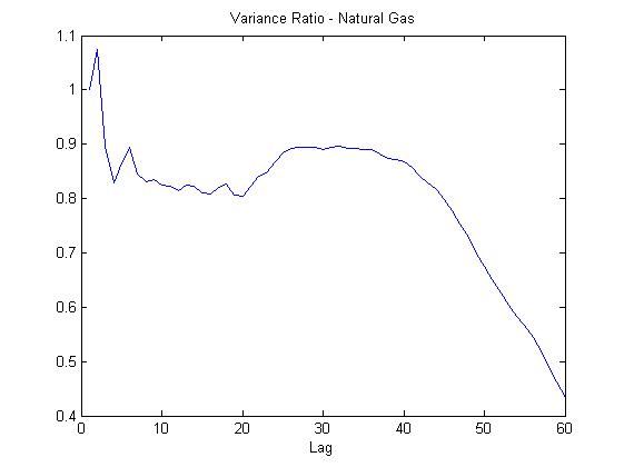
3

Executive Summary
DELTA Energy relies for its investment decisions on long-run forecasts and scenarios.
Fuel costs are an extremely important component of total costs of most energy generating
units and reliable forecasts for fuel prices are therefore needed. Besides a thorough anal-
ysis of the fuel commodity and emission allowance prices, research needs to be conducted
in the long-run availability, supply and sustainability of the various resources. Despite
of the rapid development of renewable energy sources, it is expected that in the next 30
years fossil fuels remain the main portion of power generating capacity.

The research question dealt by this report is therefore: to what extent is the long-run
behaviour of various commodities used for energy production predictable and what are
the implications for DELTA Energy’s asset investment strategy?

The focus in the research is on modelling the interdependencies of the fossil fuel price
series and assess investment implications. The main goal is to develop a framework for
DELTA Energy to simulate realistic long-run scenarios for natural gas, crude oil and
steam coal prices. Besides an application of these price scenarios is given by comparing a
coal and gas fired power plant investment.

To answer the research question quarterly price data for natural gas, crude oil and steam
coal applicable to the Northwest European region over the period 1970:Q1-2008:Q3 are
used. Predictability of the price level is tested by the Augmented Dickey-Fuller, Variance
Ratio and KPSS random walk tests. The results are not conclusive though and rule out
nor long-run mean-reversion nor the random walk hypothesis. From depletable resource
theory it can be expected that long-run prices revert in the long-run to the unobservable
marginal cost of extraction, which follows a trend and has continuous fluctuations in both
the level and slope of that trend. Deviations from that trend can be severe due to short-
run supply and demand shocks.

The prices series are modelled by a univariate stochastic long-run mean reverting model, a
vector error correction model (VECM) and a multivariate unobserved components model
(MUCM). The VECM exploits the significant cointegration relationships between the
commodities while the unobserved component models use unobserved underlying (com-
mon) factors as explanatory variables. By comparing various methodologies it is possible
to judge the models applicability, reducing model uncertainty and likewise improve fore-
casting performance.

The results indicate, especially from 1978:Q1 onward, strong cointegration between nat-
ural gas and crude oil prices and cointegration with steam coal prices as well. Deviations
from the price equilibrium however have been significant and long lasting. The univariate
stochastic long-run model is not capturing the common trend effect and therefore results
4

in unsatisfactory out-of-sample performance as a result of uncertainty in the trend param-
eter. This is evidence in favour of a multivariate approach in energy price modelling. The
VECM performs better in capturing the common trend in the long-run energy prices. A
negative trend in the long-run relationship between crude oil and natural gas versus steam
coal is identified, implying that in the long-run crude oil and natural gas are expected
to become relatively more expensive relative to steam coal. The multivariate unobserved
components model confirms these long-run relationship between the fuels without assum-
ing cointegration of the price series a priori. It seems to succeed in capturing the slow
mean-reversion to long-run equilibrium better than the VECM.

Long-run forecasts for the main energy prices are generated by multiple commercial and
government institutions. This makes it possible to compare forecasts from these insti-
tutions with the model forecasts. The fuels prices and thereby the interdependencies of
the fuels prices from the models are compared to primarily IEA forecasts from the World
Energy Outlook from 1994 onward. These results reveal that forecast performance of the
models relative to IEA predictions is mixed. It seems that IEA does not predict much
changes in the prices ratios of the fuels in most periods. The models do succeed in de-
scribing most of the fuel price interdependencies accurately. This is evidence in favour of
an approach in which the fuel prices are modelled coherently as is done in this research
using multivariate models.

High economic growth and quick depletion of crude oil reserves are the most likely ex-
planations for crude oil prices increasing more quickly than natural gas and steam coal
prices. Supply of natural gas, uranium and steam coal is currently less problematic. A
significant increase in energy demand from emerging markets could in the long-run result
in an increasing depletion rate of steam coal reserves and likewise increase coal prices.
Greenhouse gas reduction targets and emission trading on the other hand increase total
coal usage costs and can potentially decrease total steam coal demand in favour of natural
gas demand. The limited availability of natural gas reserves is an issue which could lead to
political instability and security problems resulting in supply disruptions and additional
price volatility for this commodity. From a sustainable point of view natural gas has an
absolute advantage over steam coal, which currently has higher greenhouse gas emissions
per MWh power produced. Technological developments could potentially overcome these
difficulties but will most likely increase fuel switching opportunities and further strengthen
common trends in prices as well. Uranium poses an interesting alternative to fossil fuels
as it is not associated with greenhouse gas emissions. The costs of uranium represent only
a small part of total operation costs of a nuclear power plant. Political concerns on safety
and waste disposal on the other hand make investment in nuclear power highly uncertain.

Based on the price forecasts generated by the various models and the qualitative aspects
four scenarios are constructed. By identifying these scenarios it is possible to describe
the likely future development of the fuel prices in a stylized and practical fashion. The
5

scenarios are constructed along two dimensions, energy price levels and trends in relative
prices. High versus low crude oil prices representing general energy price levels and a
stable versus a continuation of the negative trend in natural gas prices relative to steam
coal prices.

Fuel price uncertainty combined with technological change and high capital cost of invest-
ment pose an interesting challenge to energy companies willing to invest in new generating
capacity. By constructing a portfolio of assets it is possible to diversify and hedge risks
associated to this investment decision. A physical investment in a power plant is irre-
versible and can only be adjusted at the margin. The investment decision should be
based therefore not only on expectations, but on the associated risks as well. Fuel price
risk is a major component of total risk and should therefore be considered if the invest-
ment decision is made. An important result is that fuel price variance or technological
variance with respect to some technology, reduces investment in that technology. The
higher fuel price variance of natural gas is therefore an important disadvantage. If total
costs are considered though uncertainty will push towards flexible, less-capital intensive
technologies, which is in favour of natural gas fired power plants. If DELTA Energy could
reduce fuel price uncertainty by hedging or using long-term contracts then this could po-
tentially increase power plant value. Another important option is considering to delay
the investment decision until uncertainties are reduced. The described framework in this
research allows DELTA Energy to make careful investment decisions.

Given the four earlier constructed scenarios and by making assumptions for the technolog-
ical development of natural gas and coal fired power plants, it can from a costs perspective
be concluded that a coal fired power plant will probably have over the long-run the low-
est power generation costs. Only if natural gas prices are substantially lower relative to
steam coal prices or if emission costs are extremely high, natural gas fired power plants
could potentially have lower generation costs. Furthermore, the additional volatility in
natural gas prices could potentially outweigh the impact of emission price uncertainty. It
is therefore expected that the historic merit order with coal power plants having lower
marginal costs than natural gas fired power plants remains intact.

The decision for DELTA Energy to invest in a specific type of power plant depends,
besides costs, highly on the power price development. The growth of renewables and
energy savings can have a significant influence on long-run power price levels and volatility.
It is expected that renewables will increase demand for peak-load capacity which could
be generated by flexible natural gas fired power plants. A phase out of nuclear power
generating capacity on the other hand could increase demand for base-load capacity as
well. A further in detail analysis of the power market and the development of generating
capacity is therefore needed to facilitate a strategic investment decision.
6

Preface
This master thesis is the result of my efforts at DELTA Energy B.V. in Middelburg, which
started in April 2008 and is the completion of my Master of Science degree in Economet-
rics & Management Science at the Erasmus University Rotterdam.

The idea for this research came after the observation that long-run energy price assump-
tions in many energy studies and scenarios were highly influencing results and likewise
research conclusions. To improve long-term decisions making therefore in my opinion a
more in depth analysis was needed.

I would like to thank the following persons for being my supervisor: André Bosschaart at
DELTA Energy and Lennart Hoogerheide at Erasmus University Rotterdam. Also thanks
to Felix Schlichter for comments regarding my thesis and discussions about energy related
topics in general. I want to thank Koen Minderhoud for giving me the opportunity to
present my results at the Energy Forum conference about Measuring & Modelling Energy
Risk in London in November 2008. Finally, I would also like to thank Ruben van den
Berg and Pier Stapersma for feedback on this report and Robert S. Pindyck for generously
providing his dataset.

Middelburg, December 15th, 2008.

Koen den Blanken
CONTENTS                                                                                                                    7

Contents
Executive Summary                                                                                                          3

Preface                                                                                                                    6

Contents                                                                                                                   7

1 Introduction                                                                                                              9
  1.1 Context of the Research . . . . . . . . . . .    .   .   .   .   .   .   .   .   .   .   .   .   .   .   .   .   .    9
  1.2 Research Objective and Problem Statement         .   .   .   .   .   .   .   .   .   .   .   .   .   .   .   .   .   10
  1.3 Research Questions . . . . . . . . . . . . . .   .   .   .   .   .   .   .   .   .   .   .   .   .   .   .   .   .   10
  1.4 Structure and Contents of the Report . . . .     .   .   .   .   .   .   .   .   .   .   .   .   .   .   .   .   .   12

2 Data                                                                                                                     13

3 Trend line for a Depletable Resource                                                                                     17

4 Econometric Methodology                                                                                                  19
  4.1 Random Walk Tests . . . . . . . . . . . . .      .   .   .   .   .   .   .   .   .   .   .   .   .   .   .   .   .   19
      4.1.1 Augmented Dickey-Fuller test . . . .       .   .   .   .   .   .   .   .   .   .   .   .   .   .   .   .   .   19
      4.1.2 Variance Ratio Test . . . . . . . . . .    .   .   .   .   .   .   .   .   .   .   .   .   .   .   .   .   .   20
      4.1.3 KPSS Stationarity Test . . . . . . . .     .   .   .   .   .   .   .   .   .   .   .   .   .   .   .   .   .   20
  4.2 Stochastic Long-Run Mean-Reverting Model         .   .   .   .   .   .   .   .   .   .   .   .   .   .   .   .   .   21
  4.3 Vector Error Correction Model . . . . . . . .    .   .   .   .   .   .   .   .   .   .   .   .   .   .   .   .   .   22
      4.3.1 Johansen Cointegration Test . . . . .      .   .   .   .   .   .   .   .   .   .   .   .   .   .   .   .   .   23
      4.3.2 Granger Causality . . . . . . . . . .      .   .   .   .   .   .   .   .   .   .   .   .   .   .   .   .   .   24
  4.4 Multivariate Unobserved-Components Model         .   .   .   .   .   .   .   .   .   .   .   .   .   .   .   .   .   24

5 Results Forecast Models                                                                                                  26
  5.1 Random Walk Tests . . . . . . . . . . . . .      .   .   .   .   .   .   .   .   .   .   .   .   .   .   .   .   .   26
  5.2 Stochastic Long-Run Mean-Reverting Model         .   .   .   .   .   .   .   .   .   .   .   .   .   .   .   .   .   28
  5.3 Vector Error Correction Model . . . . . . . .    .   .   .   .   .   .   .   .   .   .   .   .   .   .   .   .   .   30
  5.4 Multivariate Unobserved-Components Model         .   .   .   .   .   .   .   .   .   .   .   .   .   .   .   .   .   37
  5.5 Summary . . . . . . . . . . . . . . . . . . .    .   .   .   .   .   .   .   .   .   .   .   .   .   .   .   .   .   41

6 Comparing Long-Run Forecasts                                                                                             42
  6.1 Stochastic Long-Run Mean-Reverting Model         .   .   .   .   .   .   .   .   .   .   .   .   .   .   .   .   .   44
  6.2 Vector Error Correction Model . . . . . . . .    .   .   .   .   .   .   .   .   .   .   .   .   .   .   .   .   .   46
  6.3 Multivariate Unobserved Components Model         .   .   .   .   .   .   .   .   .   .   .   .   .   .   .   .   .   49
  6.4 Conclusion and Summary . . . . . . . . . .       .   .   .   .   .   .   .   .   .   .   .   .   .   .   .   .   .   51
CONTENTS 8 7 Qualitative Aspects 54 7.1 Crude Oil . . . . . . . . . . . . . . . . . . . . . . . . . . . . . . . . . . . . 54 7.2 Natural Gas . . . . . . . . . . . . . . . . . . . . . . . . . . . . . . . . . . . 56 7.3 Steam Coal . . . . . . . . . . . . . . . . . . . . . . . . . . . . . . . . . . . 57 7.4 Uranium . . . . . . . . . . . . . . . . . . . . . . . . . . . . . . . . . . . . . 58 7.5 Emission allowances . . . . . . . . . . . . . . . . . . . . . . . . . . . . . . . 59 7.6 Summary . . . . . . . . . . . . . . . . . . . . . . . . . . . . . . . . . . . . 61 8 Scenario Analysis 63 8.1 Expert Scenarios . . . . . . . . . . . . . . . . . . . . . . . . . . . . . . . . 63 8.2 DELTA Energy’s Scenarios . . . . . . . . . . . . . . . . . . . . . . . . . . . 65 9 Investment under uncertainty 68 9.1 Real Options Theory . . . . . . . . . . . . . . . . . . . . . . . . . . . . . . 68 9.2 DELTA Energy’s perspective . . . . . . . . . . . . . . . . . . . . . . . . . . 70 9.3 Conclusion and Summary . . . . . . . . . . . . . . . . . . . . . . . . . . . 75 10 Research Conclusion 76 10.1 Problem Statement Revisited . . . . . . . . . . . . . . . . . . . . . . . . . 76 10.2 Research Conclusion . . . . . . . . . . . . . . . . . . . . . . . . . . . . . . 76 10.3 Further Research . . . . . . . . . . . . . . . . . . . . . . . . . . . . . . . . 78 References 80 A State Space format and the Kalman filter 84 A.1 Stochastic long-run mean-reverting model . . . . . . . . . . . . . . . . . . 84 A.2 Multivariate unobserved components model . . . . . . . . . . . . . . . . . 85 B Abbreviations and Definitions 86
1 INTRODUCTION                                                                            9

1     Introduction
In this chapter an introduction to the research is presented. First the context of the
research is described, followed by the research objective and problem statement. Then
several specific research questions to guide the research and their approach are formu-
lated. Finally, a short description of the structure and content of the report is supplied.

1.1    Context of the Research
Faced with ageing power utilities and increasing demand for electricity energy companies
investigate opportunities to invest in new power plants. The choice on the type of power
plant is very difficult because of uncertainty surrounding energy prices, fuel supply, regu-
lation and investment costs. Reducing these uncertainties would help energy companies to
reduce investment risk and accelerates the development of new power generating capacity.

In recent years commodity prices increased dramatically as a result of high growth ex-
pectation for the world economy and depletion of resources. Crude oil prices peaked in
July 2008 at 147 USD, but came down quickly thereafter as a result of the downward
adjustment of economic growth expectations. The high volatility in recent energy fuel
prices clearly reveals the uncertainty in fuel prices and therefore indicates the importance
for energy companies to develop a framework for long-run forecasting of energy prices.

Meanwhile, energy markets in Europe are changing rapidly as a result of market liberal-
ization and the search for alternative sources of energy. By an EU directive designed in
1996 the liberalization of the European energy market began. In January 2005 the Euro-
pean Union introduced the Emissions Trading Scheme (EU ETS) which for the first time
put a price on CO2 emissions for the power sector. Currently, the EU is considering the
emission reduction targets for 2020. Furthermore, technological developments are chang-
ing the market with, for example, the rapid growth of the liquified natural gas (LNG)
market, increased power plant efficiency and decreasing capital costs of renewables. All
these developments are further complicating the investment decision.

DELTA Energy owns several large power generating facilities and targets to expand power
generation to 2000 MW in 2015 by investing in nuclear, biomass, wind and solar power.
For the long-run DELTA wants to expand power generation capacity even further and
is continuously investigating the various investment opportunities. DELTA is already in-
vesting in a natural gas power with the construction of the Sloe plant which is expected
to be completed in 2009.
1 INTRODUCTION                                                                            10

1.2    Research Objective and Problem Statement
DELTA is planning to extend power generating capacity in the near future. To do so a
detailed analysis of the various fuel options is needed. Besides a thorough analysis of the
fuel commodity and emission allowance prices, research is conducted in the long-run avail-
ability, supply and sustainability of the various resources. The long-run in this research is
defined as the period until 2040. This is based on the assumption that the life span of a
power plant is approximately 30 years. The fuels considered in this research are: Natural
Gas, Steam Coal, Crude Oil and Uranium. The research is limited to these fuels because
fossil fuels will, despite of the rapid development of renewable energy sources, remain
the main portion of power generating capacity in the long-run as defined above. In IEA
(2008a), it is expected that by 2050 only 46% of global power in the BLUE Map (most
optimistic) scenario comes from renewables. Uranium is included in this research as well
because it is an important alternative for coal power and DELTA Energy currently has
a significant part of nuclear power in its production mix. The objective of the research
presented here is to provide DELTA Energy with insight into future developments of the
main fuels for power generation and to outline implications for DELTA Energy’s assets
and power plant investment planning decisions.

To what extent is the long-run behaviour of the various commodities used for energy pro-
duction predictable and what are the implications for DELTA Energy’s asset investment
strategy?

Fuel availability and prices may have significant impact for DELTA Energy due to changes
in the merit order of the power plants and altering operations. These effects can be direct
via higher fuel costs, for example through the purchase of coal for power plants, effecting
short-run marginal costs. Or emerging indirect via higher fuel costs effecting long-run
marginal cost and changing power plant investments. Overall, DELTA Energy’s future
asset allocation varies with the long-run outlook for the different fuels.

1.3    Research Questions
Five research questions guide the research and subsequently build a framework to handle
the problem statement.

  1. What are the long-run fuel price behaviours and their interdependencies?

  2. What are the long-run effects of availability, supply and sustainability of the fuel
     types?

  3. Which scenarios are realistic for the long-run fuel price developments?

  4. What is the effect of fuel price uncertainty on power plant investment decisions?
1 INTRODUCTION 11 5. What are the implications for DELTA Energy’s assets and investment decisions? The first research question is answered by analysing the historic price series of the vari- ous commodities. This analysis is carried out from a time series modelling perspective. First the individual commodities are analysed in univariate models. By modelling the price series development through time it is possible to better understand the historic de- velopments and to identify the key drivers. Special attention is given to the stochastic long-run mean-reverting process as suggested by Pindyck (1999). To establish this, first long-run mean-reversion opposite to the random walk has to be tested. Subsequently, an analysis of the interdependencies between the series is conducted by analysing the fuel switching opportunities, cointegration tests and by modelling the price series using vector error correction models. The second research question addresses both historic and future availability and supply limitations. Furthermore, a summarizing analysis of the sustainability of the various fuel types is presented. All these factors add insights in the risks to the use of a specific fuel and helps identifying potential structural changes in the energy market supplementing the statistical analysis. The second research question is answered using literature review and relevant expert reports. The third research question dealt with by this report is the construction of several sce- narios for the future. Using the statistical models constructed in the first section and the qualitative remarks several forecasts are generated. These forecasts are compared with other expert views and judged on realism. By doing so four plausible scenarios, which are easier to interpret, are identified. By creating these scenarios it is easier to describe the impact of long-run developments in stylized examples. The fourth research question is focused on the investment decision in a new to build power plant of given fuel type. Using the existing literature on investment under uncertainty the impact of the long-run fuel price behaviour on investment is assessed. This research question is investigated by considering several articles from portfolio and the real option theory. The fifth research question aims at answering the problem statement. The focal point lies in the impact for DELTA Energy’s assets and future investments plans. In this part specific characteristics of the Dutch Energy market are included.
1 INTRODUCTION                                                                          12

1.4    Structure and Contents of the Report
First the process of data collection and transformation is described in Section 2. Sub-
sequently, in section 3 the economic theory behind the long-run price development of
depletable resources is presented. In this way the expected behaviour and price drivers
of long-run energy prices are identified. In the econometric methodology section 4, there-
after, statistics are formulated to test these hypotheses and models are proposed to de-
scribe the long-run price paths. Results and forecasts from this analysis are given in
section 5. Thereby the first research question is answered in the results summary.

In section 6 out-of-sample forecasts from the models are compares with historic expert
views. In this way the forecasting performance of the models can be determined. To
improve current forecasts with qualitative aspects a discussion of possible future devel-
opments in the energy markets is included in section 7, answering the second research
question in the summary.

Consequently, scenarios from experts are discussed and to answer the third research ques-
tion several scenarios for DELTA Energy are formulated in section 8. The fourth and
fifth research question are answered in section 9, where the theory and consequences for
DELTA Energy of investment under uncertainty are discussed.

The conclusive answer to the research question is formulated in section 10 as well as a
discussion of the research and suggestions for further research. In the appendix a detailed
description of the state space models and the Kalman filter is presented as well as an
overview of the abbreviations and definitions used in this research.
2 DATA                                                                                    13

2    Data
Data from various sources are collected to answer the research questions as formulated in
the introduction section. In this section a brief description of the data and its origination
is given. All series are prices applicable to the Northwest European energy market. An
overview of the data and sources is given in Table 1.

Data on fuel prices were collected on a quarterly basis starting in the first quarter of 1970
till the third quarter of 2008. Quarterly data have the benefit over yearly data that it
increases the number of observations significantly. Although quarterly data potentially
induces seasonality, regressions using dummy variables for specific quarters indicate that
this effect is present but negligible, see Table 2 and 3 for results on natural gas and crude
oil. An explanation for this seasonality effect is that in the winter more natural gas is
used for heating as a result of the denser population of the Northern hemisphere. In the
summer the demand for crude oil would be higher due to holiday traffic. Increasing the
observation frequency to monthly data is not possible simply because of limited availabil-
ity of high frequency data over the entire sample period. The seasonality was removed
and the abbreviation SA was included to those series.

The prices series of the most traded fossil fuel series by DELTA Energy for natural gas,
steam coal and crude oil are used in the statistical analysis of this research. Quarterly
average prices are calculated by taking the average price over the mid-day-prices over the
months with delivery in the concerning quarter. The 1 month forward price is considered
to be a good approximation of the spot price for most commodities. In practise this implies
that to obtain for example the Q1 price the average prices of the December, January and
February contracts are used. Crude oil price data for West Taxes Intermediate (WTI) and
North Sea Brent are available over the entire sample period. The natural gas and steam
coal series from the traded data are only available starting from 2000:Q1. To obtain the
natural gas price series the Dutch gas hub prices, Title Transfer Facility (TTF), are used.
This price is over the entire sample period strongly related to the UK National Balancing
Point (NBP) and Belgium Zeebrugge (ZB) natural gas prices. For the period 2000:Q1-
2000:Q4, where data for TTF were not yet available, ZB prices were used instead. For
steam coal prices the API]2 price is used which denotes coal imported from Columbia in-
cluding freight and insurance charges for delivery in Amsterdam, Rotterdam or Antwerp.
Alternatively, API]4 for coal imports from South-Africa could have been used. The re-
lationship between these two series is extremely tight and choice of either one of these
two coal series is therefore not relevant for the long-run analysis. For crude oil North-Sea
Brent is selected as proxy for European oil prices. To cover the period 1978:Q1-1999:Q4
quarterly data from the OECD/IEA publications Energy End-Use Prices for the sector
Electricity and Import Costs and Indices by Importing Country for the Netherlands and
Belgium were used. This data is available up to current quarter and has high correlation
with the market traded series. Data over the period 1970:Q1-1977:Q4 were constructed
2 DATA                                                                                      14

      Period            Series                            Source
      Natural Gas (EUR / MWh)
      1970:Q1-1977:Q4 U.S. natural gas PPI and ECN points DOE/EIA, ECN
      1978:Q1-1999:Q4 Dutch import prices                 OECD/IEA
      2000:Q1-2000:Q4 ZB market data                      Bloomberg
      2001:Q1-2008:Q3 TTF market data                     Bloomberg
      Steam Coal (EUR / tonnes)
      1970:Q1-1977:Q4 US Coal PPI and ECN points          DOE/EIA, ECN
      1978:Q1-1999:Q4 Dutch import prices                 OECD/IEA
      2000:Q1-2008:Q3 API]2 market data                   Bloomberg
      Crude Oil (EUR / brl)
      1970:Q1-2008:Q3 Crude North-Sea Brent               Bloomberg
      Uranium (EUR / kgU), annual data
      1970-2008         NUEXCO EV (Spot)                  OECD Red Book
      CO2 Emission (EUR / tonnes), daily data
      2005-2008         EU ETS                            Bloomberg
      Producer Price Index
      1970:Q1-2008:Q3 Netherlands PPI All Items           OECD

                                Table 1: Data series and sources.

by single point observations from various sources and linked by assuming high correlation
with U.S. commodity prices indexes. The 1970:Q1-1977:Q4 price data are not used in the
ultimate model estimation and therefore only have illustrative purposes. All prices are
excluding taxes and transportation costs to the end-user.

Furthermore, for illustration annual prices of uranium were collected from the OECD Red
Book, as well as prices of emission allowances which are included in section 7. Sufficient
historic data of electricity prices are not available due to the non-existence of a free market
for electricity in Europe until the late nineties. This is also the reason why this research
focusses only on the interdependencies between the various fossil fuels without considering
the long-run relationship to electricity prices directly.

After having constructed the price series for natural gas, steam coal and crude oil from
the different sources, the series are deflated to 2008:Q1 chained euro’s using the OECD
Netherlands PPI All Items. Average annual producer price inflation in the Netherlands
over the period 1970-2008 denoted 3.0%, Figure 1. As a next step the price series, which
will be indicated by Pt , are transformed by the natural logarithm. This transformation is
done to remove skewness in the returns and to prevent models from predicting negative
values. The transformed series will be denoted by the lower case version pt . The real price
series before transformation to log prices are visible in Figure 3. The standard deviation
of the returns ∆pt over the sample period 1978:Q1-2008:Q3 are σ = 5.9%, 2.0% and 4.9%
per quarter for natural gas, steam coal and crude oil respectively.
2 DATA 15
Dependent Variable: PGASLOG
Method: Least Squares
Sample (adjusted): 1978Q2 2007Q4
Included observations: 119 after adjustments
Coefficient Std. Error t-Statistic Prob.
DUMMY*PGASLOG(-1) -0.0222 0.0113 -1.966 0.052
PGASLOG(-1) 1.0113 0.0080 126.173 0.000
R-squared 0.8335 Mean dependent var 2.3692
Adjusted R-squared 0.8321 S.D. dependent var 0.3588
S.E. of regression 0.1470 Akaike info criterion -0.9797
Sum squared resid 2.5293 Schwarz criterion -0.9330
Log likelihood 60.2919 Hannan-Quinn criter. -0.9607
Durbin-Watson stat 1.7240
Table 2: Seasonality regression - Natural Gas. The dummy is 1 in Q2,Q3 (summer) and 0 in Q4,Q1
(winter).
Dependent Variable: POILLOG
Method: Least Squares
Sample (adjusted): 1978Q2 2007Q4
Included observations: 119 after adjustments
Coefficient Std. Error t-Statistic Prob.
DUMMY*POILLOG(-1) 0.0203 0.0076 -2.684 0.008
POILLOG(-1) 0.9910 0.0053 185.316 0.000
R-squared 0.9093 Mean dependent var 3.1744
Adjusted R-squared 0.9085 S.D. dependent var 0.4369
S.E. of regression 0.1322 Akaike info criterion -1.1930
Sum squared resid 2.0434 Schwarz criterion -1.1463
Log likelihood 72.9839 Hannan-Quinn criter. -1.1740
Durbin-Watson stat 1.6416
Table 3: Seasonality regression - Crude Oil. The dummy is 1 in Q2,Q3 (summer) and 0 in Q4,Q1
(winter).2 DATA 16
Figure 1: Producer Price Index All Figure 2: U.S. dollars per euro
Items - Annual percentage change. (1970:Q1-2008:Q3).
Figure 3: Real 2008:Q1 chained quarterly prices in euro’s of natural gas, steam coal, crude oil and
uranium (1970:Q1-2008:Q3).3 TREND LINE FOR A DEPLETABLE RESOURCE 17
3 Trend line for a Depletable Resource
Price fluctuations for depletable resources are the result of shocks to supply and demand.
For a standard competitive produced good this would imply that the price in equilibrium
is equal to the marginal costs of production. Commodities though are not produced but
mined. This leaves the producer with the option to store the commodity in the ground
rather than extracting it. The price path should therefore exceed marginal costs and
follow a specific dynamic behaviour special to depletable resources, Hotelling (1931). In
this section a brief introduction to the economic theory behind price fluctuations for de-
pletable resources is given.
Price changes can emerge from fluctuations in demand, extraction costs and reserves.
These shocks affect both the log price level and its slope over time. To see this consider
the basic model of a depletable resource produced in a competitive market with constant
marginal costs of extraction c, Hotelling (1931). In his model the price trajectory, the
change of the price P through time t is dP/dt = r(P − c), where r is the interest rate or
the desired return on investment. Hence the price level is given by
Pt = P00 ert + c (1)
where P00 = P0 −c is the net price. The gap between the price Pt and the marginal costs, c,
is also known as the scarcity rent. This difference can be seen as the compensation to the
producer for selling the nonreproducible resource which leaves him indifferent between
producing now or producing in the future. At lower prices the producer could decide
that it is more profitable to store the resource in the mine or reservoir instead of selling
it to the market. If the market price is above the desired compensation than naturally
production will be increased. In principle this scarcity rent is increasing over time by the
rate of interest.
If the demand function is isoelastic, of the form Qt = APt−η then the trajectory of the
production rate is given by
Qt = A(c + P00 ert )−η , (2)
where η denotes the elasticity of demand, so the sensitivity of demand to price changes.
Using the fact that cumulative production over the life of the resource must equal initial
reserves, R0 , the initial net price can be obtained by solving
Z ∞ Z ∞
R0 = Qt dt = A(c + P00 ert )−η dt . (3)
0 0
This function can be evaluated numerically for any given value of η. If unitary elasticity3 TREND LINE FOR A DEPLETABLE RESOURCE 18
of demand (η = 1) is assumed the function reduces analytically to
A c + P00
R0 = log (4)
rc P00
or
c
P00 = . (5)
ercR0 /A −1
The price level for any time t is now given by
cert
Pt = c + , (6)
ercR0 /A − 1
with slope
dPt rcert
= rcR0 /A (7)
dt e −1
and log price trajectory
d log Pt rc
= rcR0 /A . (8)
dt (e − 1)ce−rt + c
These last three equations show that an increase in either the level of extraction costs
c, an upward shift in the demand curve A or depletion of the resources, lower R, leads
to a rise in the price level Pt , but also to increases in the slope and the log price trajec-
tory. Although the scarcity rent would in general induce an upward sloping trend it is
possible that changes in the underlying factors distort this pattern significantly. For most
depletable resources, one would expect demand, extraction costs and reserves to fluctuate
continuously and unpredictable over time. In this way it is for example possible that
an unexpected discovery of large resource fields lead to a significant drop in the scarcity
rent. Another example would be the recent unexpected high economic growth in emerg-
ing markets which has potentially let to much higher scarcity rents for various depletable
resources.
Notice that the net price level P00 is itself unobservable. This implies that if the price
level reverts to its long-term trend, which represents the long-run total marginal costs,
that this trend is unobservable. If we want to model the price process under the belief
that it reverts towards the long-run marginal cost, the marginal costs and its development
through time needs to be estimated from the data.
The next chapter introduces several econometric methodologies to test the properties of
the historic price series and model the data for forecasting purposes. These tests and
models are based on suggestions from depletable resource theory that fuel prices should
follow a long-run marginal costs based trend and have continuous random fluctuations in
both the level and slope of that trend.4 ECONOMETRIC METHODOLOGY 19
4 Econometric Methodology
In this section the various methodologies used in this report will be discussed. First in
subsection 4.1 several tests to distinguish long-run mean reversion from the random walk
are introduced. Next in subsection 4.2 the stochastic long-run mean-reverting process
is handled. Definition of the vector error correction model and cointegration testing
to determine the interdependencies between the variables are set-up in subsection 4.3.
Subsequently, as alternative in subsection 4.4 the multivariate unobserved components
model is introduced.
4.1 Random Walk Tests
The purpose of random walk tests is to determine whether or not changes in time series
are predictable. If the random walk hypothesis (RWH) is valid then the concept is that
the price serie pt wanders in an unpredictable manner. It is, therefore, for modelling
purposes extremely important to know whether series are random walk or are predictable
and consequently can be modelled using explanatory variables. The simple random walk
hypothesis without deterministic trend is defined as
E[pt ] = E[pt+τ ] and Cov(∆pt , ∆pt+τ ) = 0 ∀ t ∧ ∀ τ > 0 . (9)
Which implies that the expectation of future prices is equal to the current price and cur-
rent prices changes are uncorrelated with future prices changes for all time periods t and
lags τ . This is equal to stating that the series is covariance non-stationary or has a unit
root. Hence, the best forecast for future prices under the RWH without trend would be
the price in the current period.
Alternatively, the series is covariance stationary, has no unit root and is (long-run) mean-
reverting. To distinguish the random walk from mean-reversion the ADF, Variance ratio
and KPSS test are presented in the following subsections. Different tests are used to avoid
limitations in each of the individual tests and establish a robust conclusion.
4.1.1 Augmented Dickey-Fuller test
The Augmented Dickey-Fuller test looks whether lagged levels supply any information
helpful in explaining changes over and above that contained in lagged changes, Hamilton
(1994b). The testing procedure is based on the model
∆pt = α + βt + γpt + δ1 ∆pt−1 + . . . + δp ∆pt−m + εt , (10)
where m is the lag order of the autoregressive process. The unit root test is performed
by testing the null hypothesis γ = 0 versus the alternative hypothesis γ > 0. Critical
values can be obtained by simulation from non-standard distributions and are supplied4 ECONOMETRIC METHODOLOGY 20
by MacKinnon (1991).
4.1.2 Variance Ratio Test
The Variance Ratio test is based on work by Cochrane (1988) and Campbell and Mankiw
(1987). If the series follows a random walk then the variance of n-lags differences should
grow linearly with n.
The n-th order variance ratio is defined as
1 Var[pt+n − pt ]
V R(n) = . (11)
n Var[pt+1 − pt ]
The ratio of the variance of the 1-lag difference and n-lags difference should, if the series
is a random walk, be close to one.
4.1.3 KPSS Stationarity Test
A different approach to test the random walk hypothesis was suggested by Kwiatkowski
et al. (1992), hereafter KPSS. The difference in their approach is that they take the
mean-reversion case as the null hypothesis and the random walk as the alternative. They
take the following unobserved components time-series model as starting point, where they
decompose the series in a deterministic trend, a random walk and a stationary error:
pt = δt + rt + εt . (12)
Here rt is a random walk:
rt = rt−1 + ηt , (13)
where ηt is a stationary error as well.
Under mild regularity assumptions, they suggest that testing the null hypothesis of co-
variance stationary of the time series pt is equal to whether or not ση2 is equal to zero by
employing the test statistic:
PT
T −2 t=1 St2
LM = 2 , (14)
σˆη
In which, the partial sum process St = ti=1 ηi , where ηi is the least squares residual
P
obtained from the regression of the de-trended time series pt . Furthermore, σˆη 2 in the
denominator of equation (14) is a variance estimator that is intended to relieve the asymp-
totic distribution of the LM statistic from nuisance parameters under the null hypothesis.
As suggested by KPSS, this variance can estimated by the long-run variance estimator of
the residuals ηt .4 ECONOMETRIC METHODOLOGY 21
q−1
2
X i
σˆη = γ̂0 + 1− γ̂i , (15)
i=1
q+1
where the truncation lag q = 4bT /100c2/9 as suggested by Newey and West (1987) and
γ̂i are the i-th order autocorrelations. Critical LM values for the KPSS stationarity test
with deterministic trend are: 0.216, 0.146 and 0.119 at the 1%, 5% and 10% significance
levels respectively.
4.2 Stochastic Long-Run Mean-Reverting Model
Modelling the long-run price series for energy resources using a stochastic long-run mean
reverting process was first introduced by Pindyck (1999). Pindyck’s long-run model is
based on depletable resources theory and postulates two observations on commodity
prices:
• Reversion to an unobservable long-run marginal cost, which follows a trend;
• Continuous random fluctuations in both the level and slope of that trend.
Both observations are based on depletable resource theory as discussed in section 3.
Pindyck’s model for annual U.S. data (1870-1996) renders quite reasonable results for
crude oil, but experiences some model identification difficulties for coal and natural gas.
Later Bernard et al. (2004), using the same data set, find using Monte Carlo simulations
instabilities in the mean-reversion parameters for natural gas and coal, but not for crude
oil. Furthermore, an extension to Pindyck’s model has been developed by Radchenko
(2005) using Bayesian estimation methods and model combination, again for U.S. data.
In this research the stochastic long-run mean-reverting model is imputed with European
data and results function as reference to the alternative models of section 4.3 and 4.4.
The stochastic long-run mean-reverting process as used by Pindyck with two state equa-
tions is defined as:
pt = α1 + β1 pt−1 + φ1t + φ2t t + εt (16)
φ1t = α2 + γ1 φ1t−1 + η1t (17)
φ2t = α3 + γ2 φ2t−1 + η2t , (18)
where Pindyck sets α2 = α3 = 0, for identification of the steam coal model γ2 = 1 and for
identification of the natural gas model he removes the entire first state equation.
This model can be estimated re-writing it in state space format and applying the stan-
dard Kalman filter algorithm, Hamilton (1994a). General linear state space format is4 ECONOMETRIC METHODOLOGY 22
described in detail in appendix A. In the same appendix also the state space format of
the stochastic long-run mean-reverting model is given.
Forecasts from the model are constructed from the quarters 1998:Q3, 2003:Q3 and 2008:Q3
to reveal the effect of changes in the parameters over time. To reflect forecast uncertainty
a 90% confidence bound is used. The parameter uncertainty is simulated using 5000
simulation from the multivariate normal distribution over the parameter space. Forecast
uncertainty is simulated by random drawing from the estimation residuals.
4.3 Vector Error Correction Model
If the energy commodity prices have a common stochastic trend then it is maybe possible
to improve the forecast for these series by using a vector error correction model (VECM).
Besides by modelling the series in a multivariate model, common features can be exploited
and if cointegration exists the number of parameters to be estimated remains limited. A
common stochastic trend would give a more sophisticated way to describe the independen-
cies between the various fuels. To establish this first an investigation into the existence of
common stochastic trends or cointegration of the series has to carried out by testing for a
unit root, Granger (1981) and Engle and Granger (1987), as presented in subsection 4.3.1.
Furthermore, it is possible to include additional lags of the variables in the VECM to
explain additional variation in the returns of the series. By the Granger Causality test,
as described in subsection 4.3.2, the usefulness of this approach can be tested.
Cointegration is a familiar technique in energy price series modelling. This can be ex-
plained from economic theory by the explanation that fuels are competitive substitutes
and complements in electricity generation as well as in industrial applications. Siliver-
stovs et al. (2005), Villar and Jouth (2006), Hartley et al. (2007) and Benchivenga et al.
(2008) are just a glimpse of recent articles which find cointegration between crude oil and
natural gas prices over various time periods for U.S. and European markets. Bachmeier
and Griffin (2006) investigate, using U.S. data since 1990, cointegration of coal prices with
crude oil and natural gas prices, but conclude that these markets are weakly integrated
and therefore adjust only slowly towards long-run equilibrium.
To define the VECM, first consider the vector autoregressive (VAR) model:
Yt = µ + Φ1 Yt−1 + Φ2 Yt−2 + ... + Φp Yt−p + et , (19)
0
where in this application Yt = pt,gas pt,coal pt,oil and the Φ’s are 3 × 3 coefficient
matrices. In error correction format, that leads to the VECM
∆1 Yt = µ + Γ1 ∆1 Yt−1 + ... + Γp−1 ∆1 Yt−p+1 + ΠYt−1 + et , (20)4 ECONOMETRIC METHODOLOGY 23
where ∆1 denote first differences and where
Γi = (Φ1 + Φ2 + ... + Φi ) − Im , for i = 1, 2, ..., p − 1 , (21)
Π = Φ1 + Φ2 + ... + Φp − Im , (22)
where Π is the 3 × 3 matrix containing the information on possible cointegration relations
between the elements of Yt and I is the identity matrix. Note that due to the logarithmic
specification of the price series pt , the first differences ∆1 Yt represent quarterly returns.
Expanding parameter estimates are calculated by estimating the VECM with maximum
likelihood in Matlab version R2007a using a customized version of the LeSage Toolbox1 .
Forecasts from the VECM are constructed from the quarters 1998:Q3, 2003:Q3 and
2008:Q3 to reveal the effect of changes in the parameters over time. To reflect parameter
and forecast uncertainty a 90% confidence bound is used. The parameter uncertainty is
simulated using 5000 simulation from the multivariate normal distribution over the pa-
rameter space. Forecast uncertainty is simulated by random drawing from the estimation
residuals.
4.3.1 Johansen Cointegration Test
By first regressing equation (20) by row wise OLS, the residuals rt,1 , rt,2 and rt,3 and the
3 × 3 residual product matrices
n
X
Sij = (1/n) rt,i rt,j , for i, j = 1, 2, 3 (23)
t=1
are created. The Johansen (1988) maximum likelihood cointegration test focusses on the
rank of Π. If it is possible to construct the rows of Π by a linear combination of the
other rows the rank of the matrix is reduced. If the rank of Π = 0, all series are non-
stationary and have no common stochastic trend, but there are as many stochastic trends
as variables. If on the other hand the matrix has full rank then all series are stationary
and have no common stochastic trend as well. If a common stochastic trend or common
trends are present the rank is between these two cases. The rank r is tested by the Trace
likelihood ratio test, under the null hypothesis of the existence of at most r unit roots
and is given by
Xm
Trace = −n log(1 − λ̂i ) , (24)
i=r+1
where λi represent the i-th eigenvalue of the matrix S. A value of the test above the
critical value implies the rejection of the null hypothesis.
1
The Econometrics Toolbox by James P. LeSage is freely available at www.spatial-econometrics.com.4 ECONOMETRIC METHODOLOGY 24 4.3.2 Granger Causality Granger causality implies that a variable contains leading information on other variables. This does not mean that the variable actually drives the underlying data generating pro- cess and actually causes the other variable to change, but only in the statistical sense. It contains information in addition to the information in the series own history, which is potentially useful for forecasting purposes when specifying the correct lag structure, Granger (1969). Granger causality can be tested for normal-distributed, stationary series by regressions of the form y1t = α + β11 y1t−1 + β21 y2t−1 + . . . + βp1 y1t−p + βp2 y2t−p , for lags p = 1, 2, . . . , T , (25) where y2 is the variable that possibly Granger causes y1 . Due to the near-random walk properties of the natural gas, crude oil and steam coal series in our sample the data are transformed to first differences to construct stationarity. Sta- tionarity is required to perform the standard Granger causality test. Subsequently, the Granger causality test is performed on all six possible combinations of the three return series. 4.4 Multivariate Unobserved-Components Model As alternative to the standard cointegration analysis a multivariate unobserved com- ponents model (MUCM) can be proposed. This model can be seen as a multivariate extension of the stochastic long-run mean reverting model as defined in section 4.2. An important drawback of standard cointegration analysis as discussed in section 4.3 is that all variables constituting the stationary equilibrium relation should be included in the analysis. Additionally, Engel (2000) shows that standard cointegration tests are biased toward accepting the cointegration hypothesis in the presence of omitted integrated vari- ables. Furthermore as Morley (2007) suggests the speed of adjustment in terms of restoring their long-run equilibrium relationship is the same for all variables. That means speed of adjustment measured as the half-life response of a variable to a shock. So although for example the natural gas price adjusts in terms of magnitude more than crude oil the speed of adjustment of both is equal in the VECM. This limits the ability of the VECM to discriminate between alternative price behaviours. In Section 3 it is argued that commodity prices are determined by a combination of shocks in demand, changing extraction costs and depletion of the resource. The energy prices are in the long-run determined by changes in the underlying long-run marginal cost factors. It can be expected that changes in the marginal costs for crude oil will correspond with
4 ECONOMETRIC METHODOLOGY 25
similar hikes in marginal costs for natural gas and steam coal. For example, cost increases
in extraction costs as a result of rising building and labor costs, resource increases as a
result of intensified search by energy companies or in case of demand shocks by increased
growth of the global economy. In the unobserved components framework these omitted
integrated variables can be filtered from the long-run relations between the price series.
For the set up of the multivariate unobserved components model I follow the method-
ology in Morley (2007). He expands the work of Stock and Watson (1988) who suggest
decomposing time series into common stochastic trends (random walks) and idiosyncratic
stationary components. To apply this model to the fuel price series I add a level shift
α and the possibility to have a deterministic drift in the common stochastic trend rela-
tionship δ. The multivariate unobserved components model with p3 as base series is than
defined as
p1,t = β1 p1,t−1 + α1 + γ1 τt + δ1 t + ε1,t (26)
p2,t = β2 p2,t−1 + α2 + γ2 τt + δ2 t + ε2,t (27)
p3,t = β3 p3,t−1 + τt + ε3,t , (28)
where τt is the common stochastic trend, βi pi the idiosyncratic stationary component and
εi ∼ N (0, σε2i ). The common trend follows an unobservable random walk and is allowed
to have deterministic drift µ to capture positive growth in long-run marginal costs:
τt = µ + τt−1 + ηt , (29)
where ηt ∼ N (0, ση2 ). To allow for additional dynamics of the model, as explained in
Morley (2007), I facilitate the innovations in the MUCM to be correlated:
ρηεi = corr(ηt , εi,t ) for i = 1, 2, 3 (30)
ρεi εj = corr(εi,t , εj,t ) for i, j = 1, 2, 3 and i 6= j . (31)
For estimation, the model is casted into state space format as defined in appendix A.
Subsequently the Kalman filter and maximum likelihood estimation is applied to obtain
expanding parameter and state variable estimates. The Matlab optimisation routine for
the Kalman filter is available from the author upon request.
Forecasts from the MUCM are constructed from the quarters 1999:Q4, 2004:Q4 and
2008:Q3 to reveal the effect of changes in the parameters over time. To reflect parameter
and forecast uncertainty a 90% confidence bound is used in which the parameter uncer-
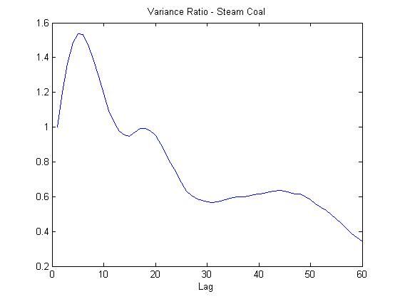
tainty is simulated using a multivariate normal distribution over the parameter space.5 RESULTS FORECAST MODELS 26 5 Results Forecast Models Results from the tests and models as described in section 4 are presented in this chapter. First the outcomes of the various random walk tests are given in section 5.1. Subsequently, in section 5.2 results from the stochastic long-run mean-reverting process, followed by the vector error correction model in section 5.3. Finally, the estimation and forecast results from the multivariate unobserved components model can be found in section 5.4. By comparing results from various models it is possible to judge the models’ applicability, reducing model uncertainty and likewise improve forecasting performance. A summary of the results and an answer to the first research question is formulated in section 5.5. 5.1 Random Walk Tests The Augmented Dickey-Fuller (ADF) unit root test for various lag lengths with determin- istic trend fails to reject the null-hypothesis of a unit root in the series. This implies that it can’t be ruled out that the series behave as a random walk. Autoregressive parameters for all series are close to one, with coal 0.98, natural gas 0.95 and crude oil 0.95. This suggests that a significantly larger sample is necessary to make rejection possible in the first place. The power of the ADF test for series with high autoregressive parameters is very limited. The failure to reject the unit root does not imply the acceptance of the random walk hypothesis. It therefore leaves the discussion open to the reader. The results of the Variance Ratio test in Figures 4, 5 and 6 for natural gas, steam coal and crude oil respectively indicate that for increasing lag differences the ratio clearly starts to deviate from 1. The decline in the variance ratio is slow, but comparable with the variance ratios found by Pindyck (1999). He also reports variance ratios of approximately 40% after 15 years (60 quarters). This is evidence in favour of long-run mean-reverting behaviour in the logarithm of the series. If we, however, test for significance of the differ- ence of the variance ratio from 1, a simple z-test fails to reject the random walk hypothesis. LM values for the KPSS test for natural gas, steam coal and crude oil are respectively 0.1116, 0.0198 and 0.0995. All values are below the 10% significance level of 0.119 and therefore indicate that there is no argument to reject the null hypothesis of stationarity. This result though can be the consequence of low rejection power of the KPSS test due to the short sample of the series. The results for crude oil deviate from Hamilton (2008) who rejects the null hypothesis for U.S. dollar prices over the sample period 1970:Q1-2008:Q1. The conclusion is that the ADF, Variance Ratio and KPSS test produce seemingly con- tradicting results. The failure to reject the unit root does not imply the acceptance of the random walk hypothesis. Nor does the failure to reject the mean-reverting hypothesis imply the acceptance of long-run memory. Therefore it is statistically impossible to rule out one of these options based on these test results.
5 RESULTS FORECAST MODELS                                              27

             Figure 4: Variance Ratio - Natural Gas, lag in quarters

             Figure 5: Variance Ratio - Steam Coal, lag in quarters

              Figure 6: Variance Ratio - Crude Oil, lag in quarters
5 RESULTS FORECAST MODELS 28
5.2 Stochastic Long-Run Mean-Reverting Model
The model as defined in section 4.2 resulted in coefficients for γ1 and/or γ2 higher than 1
for all series. This caused that the recursive estimates of the state equations can explode.
Therefore some of the γ coefficient were restricted to 1 and the models re-estimated. The
problem remained for all series and eventually all γ coefficients were eventually set to 1.
To facilitate identification the constant terms α were set to zero. Results of the remaining
parameters estimates are given in Table 4.
The Kalman filter results deviate quite substantially from Pindyck (1999). The low au-
toregressive coefficients of crude oil and natural gas suggest high mean-reversion, but
most of the variation in the log price series is captured by the unobserved components.
Remarkable is the small negative coefficient of the stochastic trend for steam coal prices,
which illustrates the slow downward moving trend in recent decades.
Forecasting results from 1998:Q3, 2003:Q3 and 2008:Q3 for natural gas, steam coal and
crude oil are given respectively in Figure 7, 8 and 9. For all three series it is clear that
the forecasted trend has changed in the recent years. This is mainly due to the fact that
the trend line depends highly on the sign of slope of the stochastic trend. For steam coal
the trend recently changed from decreasing into relatively flat.
It is clear that forecasting results from these univariate models are unsatisfactory. The
confidence intervals reveal that the uncertainty of the forecasts is very high. A small
estimation error or change in the trend parameter has a large effect on the forecasted
commodity prices. Furthermore, the model estimates give no insight in the interdepen-
dencies between the fuel prices in the long-run. This supports the multivariate approach
as followed in the subsequent sections.
Stochastic long-run mean-reverting model Estimates, 1978:Q1-2008:Q3
Natural Gas
β1 φ1,T φ2,T σε ση1 ση2 Log likelihood
0.119 1.581 0.012 0.000 0.000 0.000 60.96
(0.354) (1.826) (0.059) (0.000,0.000) (0.000,0.000) (0.000,0.000)
Steam Coal
β1 φ1,T φ2,T σε ση1 ση2 Log likelihood
0.629 1.784 -0.000 0.007 0.000 0.000 125.61
(0.241) (2.384) (0.053) (0.000,0.016) (0.000,0.000) (0.000,0.000)
Crude Oil
β1 φ1,T φ2,T σε ση1 ση2 Log likelihood
0.161 1.784 0.016 0.000 0.019 0.000 66.46
(0.377) (1.203) (0.050) (0.000,0.000) (0.003,0.100) (0.000,0.000)
Table 4: Parameter estimates calculated using MLE. Standard errors reported in parentheses.You can also read