Inequality in Exposure to Air Pollution in France: Evidence from a City-Level Public Policy
←
→
Page content transcription
If your browser does not render page correctly, please read the page content below
Inequality in Exposure to Air Pollution in France:
                   Evidence from a City-Level Public Policy†

                                 Working Paper - Preliminary Version

                                           Pascale Champalaune
                                              PSE, ENS/PSL

                                                 March 2021

                                                  Abstract

   I combine measures of neighbourhood characteristics with high-resolution remote-sensing data
   to provide the first national-scale study of cross-sectional and longitudinal inequality in expo-
   sure to fine particulate matter (PM2.5 ) in France. Descriptive evidence indicates that, at the
   national level, there is a U-shaped relationship between income and PM2.5 exposure, which is
   not reflected within urban areas. Fixed-effect models confirm that on average, higher neigh-
   bourhood income is associated with lower exposure. Both fixed-effect models and longitudinal
   inequality measures suggest that recent air quality improvements accrued predominantly to
   areas that had a lower initial exposure, and intermediate income. I then exploit a change in
   air quality schemes at the level of urban areas in an event-study framework, so as to shed
   light on potentially unequal benefits from the induced reduction in exposure. I argue that
   paying specific attention to the issue of spatial autocorrelation is crucial in a setting where
   the dependent variable is spatially continuous, and thus control for a spline of the geographic
   coordinates of census blocks in preferred specifications. I find that initially higher-income
   areas received larger benefits from the policy change, and that rural municipalities received
   larger benefits than both city centres and suburbs, a finding partly attributable to differences
   in the relative effectiveness of the implemented actions.

JEL Codes: I14, Q53, Q56, R23
Keywords: Air pollution, Environmental Economics, Inequality, Spatial autocorrelation

    †
       This work has been funded by a French government subsidy managed by the Agence Nationale de la Recherche
under the framework of the “Investissements d’avenir” programme reference ANR-17-EURE-001. I thank Lucas Chan-
cel, François Fontaine, Camille Hémet and Louis Sirugue for their time and very helpful comments and suggestions.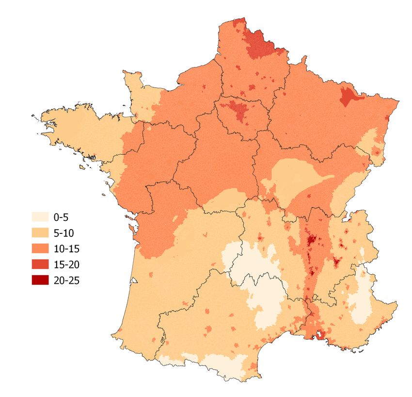
1       Introduction

As public goods, environmental amenities are an integral component of the real income of house-
holds. This makes their distribution part of the general landscape of inequality. More specifically,
unequal access to clean air may reinforce preexisting health inequalities, both across space and
across income groups. Despite both policy-makers and the general public showing growing concern
about it, the French economic literature on the issue is still in its infancy. In addition, over the
last two decades, the country recorded substantial air quality improvements, driven in part by long-
term technological development, and in part by dedicated policies. It is thus necessary to evaluate
whether the latter benefitted all individuals to the same extent.

    The contribution of this study to the academic literature is threefold. First, I provide the first
nationwide evidence of cross-sectional and longitudinal inequality in exposure to fine particulate
matter (PM2.5 ) using French data. Indeed, ever since the publication of a seminal report that
brought to light significant racial disparities in exposure to toxic waste (Chavis and Lee, 1987), and
the subsequent emergence of the environmental justice movement in the 1980s, research on environ-
mental inequality in the United States. A considerable body of literature has since unambiguously
shown that there is pervasive racial and ethnic inequality in exposure to various environmental risks
and hazards, be it from air, water or soil pollution.1
    But as opposed to the US, where the notion of environmental inequality has been part of both
the public debate and the policy arsenal for several decades, the French literature on the issue is
considerably scanter. The topic was mostly addressed by Public Health scholars, whose results
suggest that patterns of inequality may be heterogeneous across French cities. While disadvantaged
neighbourhoods appear relatively more exposed to air pollution in Marseille (Padilla et al., 2014)
or Brittany (Bertin et al., 2015), the relationship appeared to be reversed in Paris, and U-shaped
in Lyon and Grenoble (Morelli et al., 2016; Padilla et al., 2014). One of the main limitations of
most existing studies lies in their spatial scope, as to my knowledge, only two provided inceptive
evidence of nationwide disparities in exposure to ambient air pollution. First, Ouidir et al. (2017)
find a positive correlation between deprivation and particulate matter (PM10 ), nitrogen dioxide
(NO2 ), and PM2.5 exposure during pregnancy. Second, Lavaine (2015) investigates the extent to
    1
     Focusing on air pollution, it was demonstrated that both ethnic minorities and lower-income individuals face a
higher burden of exposure to Toxics Release Inventory (TRI) pollutants (Boyce et al., 2016; Zwickl et al., 2014) or
to particulate matter and ozone (e.g., Brochu et al., 2011; Muller et al., 2018) See Hajat et al. (2015) or Mohai et al.
(2009) for more comprehensive reviews.

                                                           1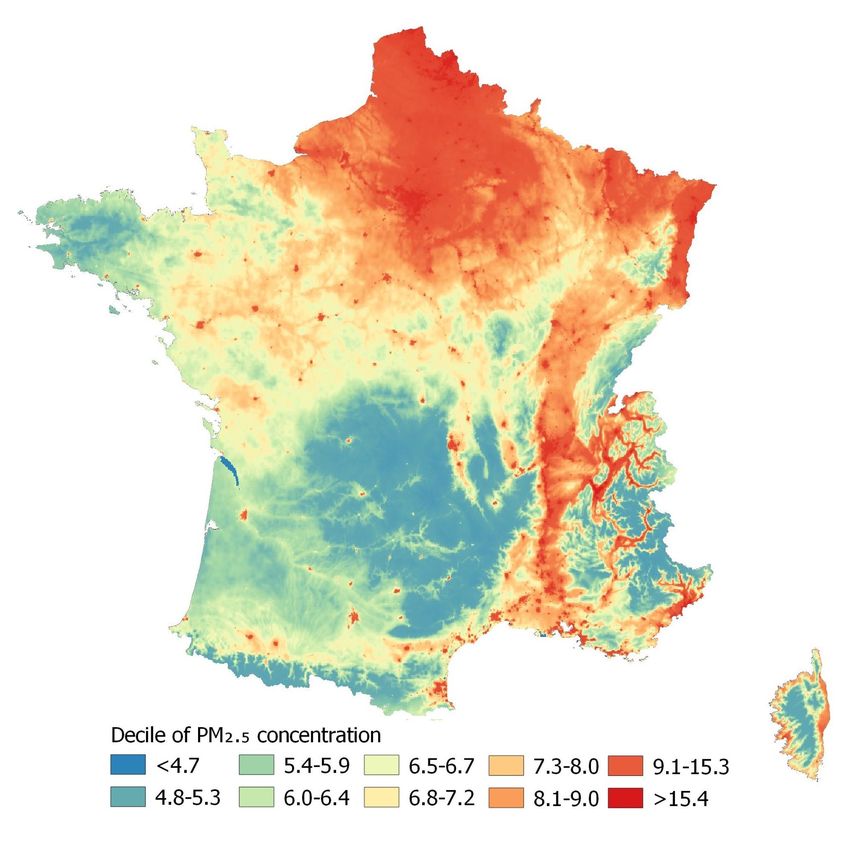
which socioeconomic characteristics and pollution levels affect the total mortality rate of French
départements, and finds that a higher NO2 concentration has a greater impact on mortality in
poorer areas than in wealthier ones. So far as I am aware, it is the only French study related
to environmental inequality that aims to determine a causal impact: the low spatial resolution is
concomitantly a weakness and a strength, as it may conceal large heterogeneity within départements,
but allows to limit bias linked to residential sorting. I thus contribute to this scarce though growing
literature by exploiting high-resolution satellite-based data, coupled with INSEE data on various
census block-level characteristics. This allows the analysis to cover the whole of metropolitan France,
and to do so at a fine spatial granularity, which constitutes an improvement as compared to previous
work on the topic.2
    Moreover, I provide the first national-scale evidence on inequality in exposure to fine particulate
matter (PM2.5 ). In mainland France, the associated health burden was recently estimated to 48,000
early deaths a year, which is equivalent to 2-year reduction of life expectancy at 30 on average
(Medina et al., 2016). Albeit these detrimental health impacts, this pollutant has been overlooked
by the French literature on environmental inequality, partly due to the fact that there were very
few PM2.5 monitors prior to the 2010s. I thus contribute in filling this gap.
    I show that, at the national level, there is a U-shaped relationship between PM2.5 exposure
and income, which is not reflected within urban areas, where only the lowest income deciles face a
disproportionate burden of exposure. In a next step, I tackle the omitted variable bias related to
unobserved neighbourhood heterogeneity using fixed-effect models, and confirm that there is indeed
a negative relationship between the two variables of interest in France. Potential explanations are
selective firm siting, selective neighbourhood sorting, and a market-like combination of the two
(Banzhaf et al., 2019). The results also suggest that the share of immigrants is positively associated
with PM2.5 concentration, hinting at an ethnic gap in exposure reminiscent of that observed in the
United States. I also contribute to the literature by providing longitudinal measures of inequality,
and present evidence that census blocks that benefitted from the smallest air quality improvements
are those that had the highest initial exposure, and that were located either at the lower or upper
end of the distribution of income. This study thus uncovers that despite the fact that PM2.5
exposure dropped throughout the country between 2006 and 2016, there is growing inequality in its
distribution.

    2
     A high spatial resolution helps limit the risk of ecological fallacy, i.e., so as to avoid making erroneous inference
on individual correlations based on neighbourhood correlations (Banzhaf et al., 2019).

                                                            2
My second contribution consists in taking advantage of a policy change that occurred at the level
of urban areas, in order to investigate whether new PM2.5 regulation played a role in this evolution.
In France, since the 1996 LAURE law, part of the regulation of air quality occurs at the level of
urban areas, through mandatory Plans de Protection de l’Atmosphère (PPA). To this date, about
half of the metropolitan French population lives in a zone covered by a PPA, which make it a flagship
policy. The 2008 EU Directive on cleaner air for Europe incorporated fine particulate matter as a
newly regulated pollutant. As a consequence, urban areas were required to introduce new air quality
schemes, so as to introduce measures aimed at reducing PM2.5 concentration. Given that the years
of implementation vary from 2012 to 2016, I make use of an event-study design in order to analyse
how inequality in exposure to air pollution evolved as a consequence of this change. I demonstrate
that these revised plans predominantly benefitted initially advantaged neighbourhoods, i.e., those
whose income lay above the median. In addition, I provide quantile regression estimates which
suggest that lower quantiles of exposure received larger air quality improvements.
   In line with this finding, I show that rural areas benefitted from a greater decrease in exposure
than city centres and suburbs. I argue that this is due to differences in the relative effectiveness
of the actions taken in rural areas, as opposed to urban ones. On the one hand, measures aimed
at reducing air pollution in large cities often prove less effective as hoped ex ante. For instance,
Bou Sleiman (2021) shows that the pedestrianisation of a Parisian riverbank in September 2016
induced a decrease in air quality in nearby areas. Indeed, despite the simultaneous implementation
of a mix of policies, air pollution peaks are still common in the French capital (Font et al., 2019).
On the other hand, the replacement of old furnaces by new models of lower emission intensity, which
is mostly done in rural areas, or the prohibition of open burning of waste appear more effective,
since these sources account for a larger proportion of total emissions (Citepa, 2018).

   As a third contribution, I pay specific attention to formally accounting for spatial autocorre-
lation. Indeed, if emissions decrease in a neighbourhood i while they remain constant in a neigh-
bourhood j, air pollutant concentration will decrease in both neighbourhoods. This means that,
when studying the impact of the implementation of Plans de Protection de l’Atmosphère, or any
similar policy, relative neighbourhood location acts as a catalyser of the effects. Yet, this issue has
been largely overlooked by the economic literature on environmental inequality. Concomitantly, I
provide a concise review of the methods used in existing studies, and argue that the spatial lag
model, which seems the most widespread (see, e.g. Havard et al., 2008; Verbeek, 2019), relies on

                                                  3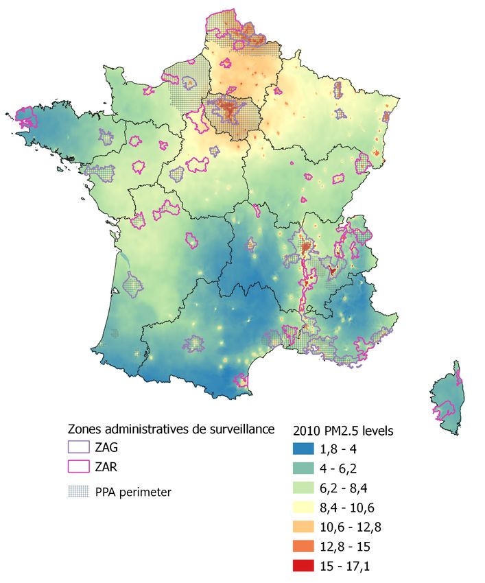
arbitrary parametric assumptions that may threaten the validity of the estimates. I thus rely on
a non-parametric approach to model spatial autocorrelation, using a smoothing spline of census
block geographic coordinates (Wood, 2017). I show that after controlling for neighbourhood loca-
tion, while the pollution-income relationship remains similar, there is a stronger positive correlation
between the share of immigrants and PM2.5 exposure. The sensitivity of the results to controlling
for neighbourhood location is therefore consistent with observed segregation patterns.

    The remainder of this paper is organised as follows. Section 2 presents the data on neighbourhood
characteristics and fine particulate matter concentration. Section 3 describes the cross-sectional pat-
terns of inequality in exposure to PM2.5 in France, first using graphical evidence, then providing
evidence on the evolution of these inequalities, using both vertical and horizontal equity measures. I
then turn to fixed-effect models and study their sensitivity to controlling for spatial autocorrelation.
Section 4 describes the French air quality regulatory context, while Section 5 presents the identi-
fication strategy used to study the impact of the revision of Plans de Protection de l’Atmosphère
(PPA). Section 6 presents the main results, and underlines the importance of the use of a spatial
model. Section 7 studies the heterogeneity of the effects, based on quantile regression estimates and
subsample analyses. Section 8 concludes.

2     Data

2.1   Income and neighbourhood characteristics

I make use of IRIS-level data made publicly available by INSEE, the French National Institute for
Statistics and Economic Studies. IRIS (Ilôts Regroupés pour l’Information Statistique, or aggregated
units for statistical information), the equivalent of American census blocks, were designed by INSEE
so as to prepare for the dissemination of the data collected through the 1999 Census. They were
built using criteria based on both administrative boundaries and demographic characteristics, so as
not only to be tractable in the long-term, but also to constitute a homogeneous fraction of a mu-
nicipality in terms of housing and land use. There are 3 categories of IRIS, starting with residential
IRIS (habitat), which are home to between 1,800 and 5,000 inhabitants and make up 92% of the
total number of IRIS. Business IRIS (IRIS d’activité) cluster at least 1,000 workers, and no less than
twice as many workers as inhabitants. Finally, miscellaneous units (divers) are large and specific
areas that are sparsely populated, such as parks, forests or harbours, and represent 3% of IRIS. To

                                                   4
this day, all cities that are home to more than 10,000 inhabitants, and the majority of municipal-
ities with 5,000 to 10,000 inhabitants are divided into IRIS. By extension, and so as to cover the
entire French territory, every municipality that is not divided into IRIS is considered as an IRIS.3 In
2017, there were on average 1,381 inhabitants per unit when counting all municipalities, and 2,744
when focusing on cities divided into IRIS. Using my sample restriction, whereby I drop units whose
population is below a threshold of 200 inhabitants, these averages are, respectively, 1,663 and 2,863.
Putting restricted-access databases aside, this is the finest spatial unit of observation available in
French data. Finally, during the study period, IRIS and municipalities underwent several changes,
especially due to the fact that municipality mergers were common from 2015 on. I provide details
on the methodology used to obtain a spatially consistent set of census blocks in Methodological
Appendix A.1, as well as a categorisation of the sample of census blocks using different typologies
(e.g., urban-rural, centre-suburbs) in Table 7 of Appendix B.

    In addition to income, the main variable of interest that I extract from INSEE data, I select
several neighbourhood characteristics listed in Table 5 in Appendix B. These variables were first
selected based on theoretical grounds, in the sense that they could be potential confounders in the
pollution-income relationship that I study in Section 3. Moreover, epidemiological studies on social
disparities in health and on environmental inequality generally rely on the European Deprivation
Index (EDI) as a measure for the degree of neighbourhood precariousness (e.g., Morelli et al.,
2016; Ouidir et al., 2017; Padilla et al., 2014). The variables included in this index are those that
are the best predictors of both objective and subjective poverty measures within each European
country. I thus add as controls those found by Pornet et al. (2012) to best mirror individual
deprivation in France. In addition to the descriptive list provided in Table 5, summary statistics of
all neighbourhood characteristics for all years within the study period, which extends from 2006 to
2017, are available in Table 6 in Appendix B. Note that the median of census block median incomes
amounts to e19,3124 , which is approximately equal to the French median income throughout the
period (e19,270 in 2010). However, due to the difference in observation level, the first decile of
income is for instance equal to e16,162 in 2017 in my data, as opposed to e11,040 based on
individual-level data (Argouarc’h and Picard, 2018).
    3
      Hereafter, I use the terminology of “municipality IRIS” for municipalities that are either not divided into IRIS
or those that are, but had less than 10,000 inhabitants at least once during the study period, which implies that
income is only provided at the municipality level. In contrast, the words “IRIS” or “census block” are used to define
the observation level, regardless of the type of municipality it refers to.
    4
      All values are given in 2019 constant euros.

                                                          5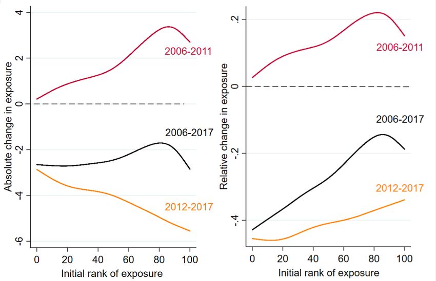
2.2    Fine particulate matter concentration and exposure

I use PM2.5 concentration data from the Atmospheric Composition Analysis Group (ACAG) in
Dalhousie University, Canada, and Washington University in St. Louis. The researchers exploit
both remote-sensing sources and ground-level monitor data gathered by the European Environment
Agency (EEA) in order to deduce the spatial distribution of fine particulate matter throughout
the whole of Europe. They make use of GEOS-Chem, a recent chemical transport model that was
jointly developed by the ACAG and Harvard University researchers.5 I observe PM2.5 concentration
for years 2001 to 2017. The yearly files are made available to the public in raster format in grids of
.01◦ × .01◦ , i.e., approximately 1.1 km × 1.1 km at the equator. This means that each pixel located
in Paris has a West-East side of around 650 m, and a North-South side of around 1.1 km. Note that
the degree of precision of this data appears to be primarily adapted to large-scale studies like this one.

   I infer pollution concentration at the census block level by computing the weighted average
of the level of pollution associated with each raster grid that (at least partly) overlaps with each
census block, using the Zonal Statistics plugin of QGIS. This implies that exposure is defined as the
mean of the values of the raster grids at least part of which are inside the boundaries of each IRIS,
weighted by the proportion of the area of the grid present within the area of the IRIS. Fowlie et al.
(2019) highlight that satellite-based predictions of pollution concentration, though more spatially
resolved and reliable than monitor data, can suffer from a certain degree of forecast error, especially
at extreme values. Given that the ACAG data I make use of is calibrated at the European level, and
that France has overall intermediate levels of air pollution compared to its European neighbours
(for instance, compared to Poland or the Pô Valley), this issue is not much of a concern in this
study. Still, the spatial extent of census blocks implies that there is some measurement error of
the pollution exposure variable. Indeed, as exposed in Section 2.1, not all French municipalities are
divided into IRIS, and the average surface area of a French commune is 14.88 km2 (14.83 in my
data). This is small compared to most European countries, but remains an issue in this context:
on average, 17.71 grid points were used to compute average concentration for municipality IRIS,
while only 2.15 were used in the case of “real” IRIS. Therefore, although it is not too concerning,
the independent variable is subject to measurement error, which reduces the power of the statistical
tests conducted in following sections, or, in other words, increases the risk of Type-II error.

   5
    Further information relative to the GEOS-Chem transport model is available on the dedicated website: http:
//acmg.seas.harvard.edu/geos/.

                                                      6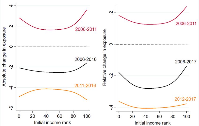
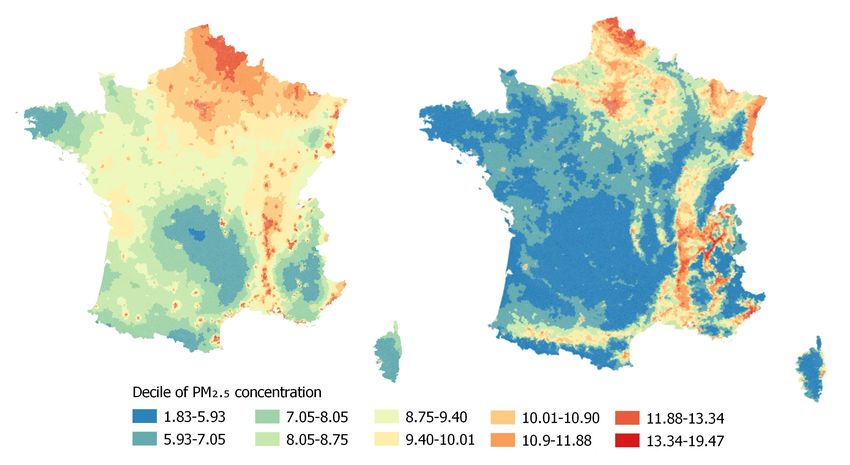
Figure 1: PM2.5 concentration and median income by decile – 2017

                   (a) PM2.5                                               (b) Median income

Sources: Author’s computations based on data from the ACAG (left) and INSEE (right).
Similarly to the EU Average Exposure Index (AEI) definition, 2017 PM2.5 concentration is defined as the mean of
the 2016, 2017 and 2018 PM2.5 concentrations.

    I define average exposure as the population-weighted mean PM2.5 concentration within a given
IRIS. Census block-level data, including population data, are not available for years prior to 2006.
These data constraints imply that the analysis focuses on the 2006-2017 time period. According
to the data, average exposure to fine particulate matter is equal to 9.19 µg/m3 in 2017, which
complies with both the European limit value of 25 µg/m3 and the World Health Organisation
(WHO) guideline of 10 µg/m3 , on average. However, the distribution of PM2.5 concentration ranges
from 1.83 to 17.15 µg/m3 at the IRIS level. I provide comparisons of the ACAG data to some other
sources in Methodological Appendix A.2.

3     Descriptive evidence

3.1     Graphical evidence

3.1.1    Patterns of inequality

Starting with macro-scale patterns of inequality in exposure to fine particulate matter, Figure 1 de-
picts PM2.5 concentration by decile alongside a map of median income by decile and by département.
The latter administrative division roughly corresponds to the county level of the United States or

                                                      7
the United Kingdom. Comparing these two maps shows that, in France, even focusing on the re-
gional scale and avoiding delving into urban area-specific heterogeneity, the relationship between
PM2.5 exposure and income is not at all monotonic. Île-de-France (excluding Seine-Saint-Denis) and
the former Rhône-Alpes region combine some of the highest levels of both fine particulate matter
exposure and income, while, unsurprisingly, the association is reversed for the rural areas of central
France. On the other hand, the northern départements of Nord, Pas-de-Calais, Aisne and Ardennes
belong to the highest decile of exposure and the two lowest deciles of income. On the other side of
both spectra, the Atlantic South-West and Brittany compound relatively high income and low ex-
posure. These differences cannot simply be explained by the presence of major cities, which usually
couple comparatively higher pollution and higher income, as the situation in the north of France
strongly contradicts this argument.

   Turning to census block-level information, Figure 2a displays the unconditional average exposure
to PM2.5 as a function of a neighbourhood’s decile of income, for all even-numbered years of the
study period. It appears that the relationship between neighbourhood median income and PM2.5
concentration follows a U-shaped relationship. The average exposure of the top-10% neighbourhoods
is lower than that of those located at the 9th decile of income, and similar to that of the bottom 10%.
This is consistent with the fact that, in France in 2012, 65% of individuals living below the poverty
line lived in large urban centres (INSEE’s grands pôles urbains), and 20% in the Paris urban area
(Aerts et al., 2015), where fine particulate concentration is higher. More generally, this U-shaped
curve reflects the characteristics of most French urban areas: albeit different levels of residential
segregation, statistically more polluted city centres and inner suburbs usually compound both high-
and very low-income neighbourhoods, while peri-urban neighbourhoods have more intermediate
levels of income, and are increasingly well-off (Aerts et al., 2015; Floch, 2014, 2017).
   However, conditioning PM2.5 concentration on urban area yields a completely different story, as
shown in Figure 2b: within urban areas, neighbourhoods with very low income are considerably more
polluted than their wealthier counterparts. Indeed, in 2017, 60% of the neighbourhoods located in
the bottom 10% of the income distribution (i.e., below e16,162) are exposed to PM2.5 levels that
are above the WHO standard of 10 µg/m3 , while, conversely, 80% of the neighbourhoods of the
next 10% comply with this standard (as can be deduced from the CDFs in Figure 15 of Appendix
B). Average exposure roughly decreases with income up to the 9th decile, and then slightly rises
with income at the very right end of the distribution. Notice also that conditionally on urban area,

                                                  8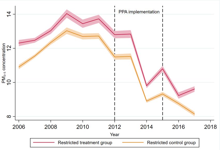
Figure 2: Average exposure to PM2.5 as a function of income decile

                     (a) Unconditional                            (b) Conditional on urban area

                                         (c) Conditional on urban unit

Note: Panel (a) displays the raw relationship between PM2.5 concentration and neighbourhood income decile. Panels
(b) and (c) display the residuals of regressions of PM2.5 concentration on an urban area dummy variable and on an
urban unit dummy variable, respectively. An urban area (INSEE’s aire urbaine) comprises peri-urban municipalities,
whereas urban units (INSEE’s unités urbaines, commonly called agglomérations in French) only comprise city centres
and suburbs.

the exposure of census blocks located in the top 40% of the distribution of neighbourhood income is
substantially lower than the average, while the 4th and 5th deciles have average exposure. Finally,
Figure 2c focuses on what happens within urban units, that is, within city centres and their close
suburbs. In other words, it excludes peri-urban areas. As a consequence of the abovementioned
phenomenon that relates income to location in France, there is less variation in the residual PM2.5
after controlling for the urban-unit dummy than when controlling for an urban-area dummy, and
the relationship is more linear. In any case, this graph also hints at a negative relationship between
neighbourhood income and fine particulate exposure.

                                                        9
The negative relationship between census block median income and exposure to fine particulates
holds in most of the 12 largest French urban units, as shown in 16 in Appendix B. It is particularly
strong in Marseille and Toulon, and a bit less so in Toulouse and Grenoble. While exposure mono-
tonically decreases with income in the Paris urban unit, i.e., in Paris and its inner suburbs (petite
couronne), when one broadens the scale and looks at the urban area, which covers the whole of
Île-de-France, the relationship is U-shaped, which can be explained by the fact that its peri-urban
neighbourhoods have intermediate median income.
3.1.2 Evolution in exposure
Figure 3 displays the evolution of average exposure to fine particulate matter in metropolitan France
throughout the study period. According to this figure, average exposure increased from 11.89 µg/m3
in 2006 to around 14 µg/m3 in 2009-2011, before falling to 9.19 µg/m3 in 2017. Hence, for years
2014 and 2016-2017, according to matched ACAG and INSEE data, exposure seems to be line with
the World Health Organisation (WHO) guideline of 10 µg/m3 , on average. Average exposure fell
by 5.02 µg/m3 , or 35.3%, between the peak year 2009 and 2017, a decrease similar to the United
States’ in the 2000-2014 period (Currie et al., 2020; Voorheis, 2017).
However, this national average masks some considerable spatial disparities in the evolution of
fine particulate matter concentration. Figure 4 shows PM2.5 concentration in 2006 and 2017, i.e.,
the first and last years of the study period, by decile of the total distribution across these two
Figure 3: Evolution of average exposure to PM2.5 – 2006-2017
10Figure 4: PM2.5 concentration by decile – 2006 and 2017
(a) 2006 (b) 2017
blablablablablablablablab
years. In 2006, the least exposed areas were Massif Central, the Pyrénées, the southern part of the
Bay of Biscay and the tip of Brittany, and remain so. More specifically, PM2.5 concentration was
already very low in Massif Central, and did not significantly decrease, while it did in the last three
regions. On the other hand, the northern part of the country, the Paris region and the Rhône Valley,
which were located in the top 30% of the distribution in 2006, stayed at this position in 2016. This
implies that while pollution was already high in these areas, and particularly much higher than the
WHO guideline, they remained at the top of the cross-year pollution distribution, while the rest of
the country moved down. Taken together with the map of Figure 1b, this does not allow to draw
clear-cut conclusions on longitudinal patterns of inequality at the macro-level: while the low-income
northern départements remained polluted, high-income ones like Rhône or Seine-et-Marne also did.
3.1.3 Pollution-reduction profiles
In order to analyse longitudinal inequality in exposure to PM2.5 , I proceed to compute pollution-
reduction profiles, following Voorheis (2017), who argues that, although there is a sizeable body
of literature providing cross-sectional measures of environmental inequality in the US, much less
11is known about longitudinal environmental inequality. As such, he adapts a method used in the
literature on intra-generational mobility and first proposed by Jenkins and Van Kerm (2006), called
income-reduction profiles, to pollution exposure. The resulting pollution-reduction profiles (PRP)
allow to capture both vertical equity concerns (i.e., how PM2.5 exposure varies across initial ranks
of exposure) and horizontal equity concerns (i.e., how PM2.5 exposure varies across initial ranks
of income). Both types of PRP are also computed both in absolute terms, using the difference
between exposure in year t + x and exposure in year t, and in relative terms, using the difference
between the logarithm of exposure in year t + x and that of year t. As shown in Figure 3, average
exposure increased between 2006 and 2011, and decreased ever since. This framework thus allows
to visualise the distributional impacts of the 2006-2011 air quality deterioration and the 2012-2017
(and overall) air quality improvement. All PRP are obtained by fitting a thin plate regression spline.
Figure 5 (resp., Figure 6) shows the vertical (resp., horizontal) equity profiles, with absolute
changes in exposure on the left-hand side and relative changes in exposure on the right-hand side.
Between 2006 and 2017, regardless of their initial level of exposure to PM2.5 , on average, neighbour-
hoods benefitted from overall quite comparable decreases in absolute terms, between -1.7 µg/m3
and -2.8 µg/m3 . However, this implies that, in relative terms, census blocks that were initially less
exposed to PM2.5 benefitted from larger improvements than those who were initially more exposed.
Distinguishing between the two phases of the study period, the graph suggests that initially dis-
advantaged census blocks experienced a higher increase in exposure between 2006 and 2011, and a
smaller relative decrease in exposure after 2011, compared to their initially less exposed counter-
parts. In particular, neighbourhoods at the 10th percentile of initial exposure were subject to a 40%
decrease in exposure, against a 14% decrease at the 90th percentile. In short, the vertical equity
measures suggest that both the rise and the fall in PM2.5 concentration have been regressive, with
larger benefits accruing to initially less exposed areas.
This is consistent with what Figure 3 shows at a larger geographical scale: while PM2.5 con-
centration decreased throughout metropolitan France, regions that were initially the most polluted,
such as Hauts-de-France and Île-de-France, did not experience larger relative decreases than others.
This may partly be attributed to relatively smaller decreases in emissions due to less effective poli-
cies, but another potential explanation for this may be that fine particulate matter concentration
did not decrease more in initially more polluted areas because a potentially significant part of these
particles is imported. Indeed, PM2.5 can travel long distances, which implies that a potentially
12Figure 5: Pollution-reduction profiles – Vertical equity
Note: The initial rank of exposure is the rank in the distribution of IRIS exposure to PM2.5 in 2006.
non-negligible part of neighbourhoods’ observed concentration is not due to domestic emissions.
For instance, in Île-de-France in 2010, it was estimated that 39% to 68% of their observed quantity
was produced outside the region (Airparif, 2011).
Turning to the horizontal equity measures of Figure 6, the first finding is that, similarly to verti-
cal equity measures, absolute changes in exposure over the whole study period were rather uniform
across the initial income distribution. But again, in relative terms, the bottom decile of initial
income, i.e. neighbourhoods with a median income of e14,300 in 2006, received a 20% decrease
in exposure, while those at the 4th decile (e17,360), received the largest relative decrease of 28%.
Neighbourhoods of the top 10% of income (whose 2006 income is above e24,000) benefitted from
the smallest relative improvement, with a 17% average decrease. To summarise, in relative terms,
it appears that the pollution-reduction profile is U-shaped, with air quality improvements accruing
to a greater extent to neighbourhoods located in the middle 60%, while those at either end of the
income distribution experienced significantly smaller relative decreases. Splitting the study period
into two phases, it appears that the bottom 20% and the top 20% of income not only experienced
the largest (relative or absolute) increase in exposure between 2006 and 2011, but also slightly
13Figure 6: Pollution-reduction profiles – Horizontal equity
Note: The initial income rank is the rank in the distribution of IRIS median incomes in 2006.
smaller relative decreases after 2011. Taken together with the evidence in Figure 5 and Section 3.1,
these patterns are consistent with an overall improvement in air quality throughout the country,
which, however, favoured municipalities and neighbourhoods that combine intermediate income and
comparatively low pollution levels. This implies that although overall PM2.5 exposure underwent a
substantial drop during the study period, inequality in exposure intensified.
A small counterfactual exercise can highlight the potential role played by relative mobility across
neighbourhoods. Indeed, one can compute the average exposure of neighbourhoods in 2017 using
their 2006 rank, and compare it to the actual average. With this definition, the average of exposure
of the bottom 10% of 2017 in 2017 is 11.30 µg/m3 , but that of the bottom 10% of 2006 in 2017
would have been 11.08 µg/m3 , holding the ranks fixed. On the other end of the spectrum, the 2017
top 10%’s average exposure is equal to 10.86 µg/m3 , while it should have been 11.01 µg/m3 holding
the ranks fixed. As such, the bottom 10% of 2017 is more exposed than the 2006 bottom 10%
would have been, and the reverse holds for the top 10%. This implies that neighbourhoods that
are “new” to the bottom 10% are more polluted than those that “left” the bottom 10%, and that
neighbourhoods that are “new” to the top 10% are less polluted than those that “left” the top 10%.
14Such a fact is consistent with relative mobility patterns that would occur due to the neighbourhood
sorting mechanisms, where higher-income (resp., lower-income) individuals would self-select into
cleaner (resp., more polluted) neighbourhoods, be it due to pollution-related out-migration or to
market forces (Banzhaf and McCormick, 2012; Banzhaf et al., 2019). Individual data would be
needed to formally test these hypotheses.
3.2 Fixed-effect models
I provide a formal analysis of the correlation between fine particulate matter exposure and neigh-
bourhood income by running IRIS-level fixed-effect models. By doing so, I exploit the variation in
income and PM2.5 concentration within census blocks, and thus difference out the potentially con-
founding effect of unobserved census block-level characteristics which could influence the location
decision of individuals. Indeed, solely controlling for a series of neighbourhood socio-demographic
characteristics (listed in Appendix Table 5) does not tackle the potential bias arising from the qual-
ity of the amenities present within or in the vicinity of neighbourhoods. These are particularly
important in this study due to the fact that households may substitute away air quality for other
amenities, such as cultural facilities, schools or proximity to large business districts. Although it is
not discussed, this omitted variable bias is present in any of the abovementioned cross-section analy-
ses (e.g., Ouidir et al., 2017; Zwickl et al., 2014), whose model identification relies on cross-sectional
variations. The corresponding equation is the following:
ln(PMit ) = α + βIN C ln(INCit ) + βX Xit + λt + νi + εit (1)
PM2.5 exposure is right-skewed, so I take its natural logarithm in all regressions. ln(PMit ) corre-
sponds to the (log) average exposure in census block i, during year t. ln(INCit ) is the median income
of census block i in year t. Xit includes the covariates taken from the list displayed in Table 5 in
Appendix. I include the share of inhabitants that undertook higher education, since more educated
individuals may attach a higher value to air quality than less educated individuals, and thus hold a
different view of the trade-off between amenities and air pollution, which influences their residential
choice. For similar reasons, I select the shares of population by occupation, divided in 8 categories
(see Appendix Table 5). Moreover, homeowners and subsidised housing tenants, i.e., those who
live in HLM (Habitation à Loyer Modéré), may have more stringent residential mobility constraints
than tenants of privately owned dwellings, which would prevent them from leaving polluted areas.
15I also control for the share of dwellings that are not equipped with electric heating, since domestic
wood burning is one of the main sources of PM2.5 in France (Citepa, 2018), and similarly for the
share of households that own a car. The fractions of immigrants, of unemployed individuals, and
single-parent households are also used as measures of deprivation (Pornet et al., 2012). In preferred
regressions, Xit also includes a spline of the geographic coordinates of the centroid of census block
i, which can be denoted s(xi , yi ), with xi the longitude and yi the latitude of said centroid. This
amounts to switching from a standard OLS model to a Generalised Additive Model, which allows
me to formally take into account the issue of spatial autocorrelation. In OLS models, standard er-
rors are clustered at the urban-area level: this means that spatial correlation is modelled discretely,
since it is designed to follow urban area boundaries. Pollution, however, is distributed continuously
across space. As a consequence, pollution levels on either side of an urban area boundary are thus
as likely to be correlated as pollution levels of two census blocks located within the same zone. This
argument also holds for income, the variable of interest, as well as other neighbourhood charac-
teristics. Hence, the residuals of equation (1) are most likely not independently distributed when
omitting to control for s(xi , yi ). I further discuss this issue in Section 5.3. Finally, I cluster standard
errors at the urban-area level in standard OLS regressions, and weight all regressions by population.
I take advantage of the panel structure of my data to deal with the omitted variable bias related
to time-invariant unobserved IRIS-level characteristics, and I add year fixed effects in order to tackle
the impact of year-specific shocks that would impact both income and PM2.5 concentration, such
as a shock in economic activity. However, it is likely that there are remaining biases, meaning that
the models do not identify a causal impact. First, the models rely on the assumption that there
exists no time-varying unobserved heterogeneity across IRIS throughout the 2006-2016 time period,
since it was computationally inaccessible to introduce more than 400,000 time-varying fixed effects.
Second, unlike an individual-level fixed-effect model, the models that I estimate do not fully tackle
the self-selection issue that is inherent to the study of environmental inequality. Indeed, they do
not resolve the potential reverse causality of the pollution-income relationship,6 which opposes the
neighbourhood sorting hypothesis to the firm siting hypothesis. As a consequence, the test that I
provide here boils down to looking at whether any of these two hypotheses, or a combination of the
two, may be verified in France.
6
Lagged independent variables are not particularly helpful in this context, given the degree of inertia of the
variable of interest between 2 subsequent years of observation at the IRIS level.
16Table 1: Fixed effect models – Partial results
OLS regressions Spatial GAM regressions
(1) (2) (3) (4) (5) (6)
Variable
-1.279∗∗∗ -0.229∗∗∗ -0.194∗∗∗ -1.297∗∗∗ -0.229∗∗∗ -0.170∗∗∗
(Log) income
(0.117) (0.029) (0.025) (0.002) (0.001) (0.001)
0.187∗∗∗ 0.197∗∗∗
% Immigrants
(0.028) (0.001)
0.209∗∗∗ 0.217∗∗∗
% Tertiary-educated
(0.040) (0.002)
0.268∗∗∗ 0.274∗∗∗
% White-collar
(0.083) (0.004)
-0.163 -0.174∗∗∗
% Unemployed
(0.129) (0.006)
0.062∗ 0.067∗∗∗
% Social housing
(0.032) (0.002)
15.055∗∗∗ 4.676∗∗∗ 4.166∗∗∗ -0.000∗ -0.016∗∗∗ -0.008∗∗∗
Intercept
(1.152) (0.289) (0.257) (0.000) (0.001) (0.001)
Year fixed effects X X X X
R2 within 0.28 0.77 0.78
R2 between 0.01 0.01 0.30
R2 overall 0.00 0.22 0.47 0.28 0.77 0.78
# Observations 440,490 440,490 440,490 440,490 440,490 440,490
# Groups 37,500 37,500 37,500 37,500 37,500 37,500
Note: All regressions are weighted by 2017 population. Standard errors clustered at the urban-area level are displayed
in parentheses. ∗ : 10% level, ∗∗ : 5% level, ∗∗∗ : 1% level.
Columns (1)-(3) present the results of the OLS regressions, while Columns (4)-(6) present the results of the spatial
GAM regressions, which control for a spline of the geographic coordinates of the census block. The number of
observations corresponds to N × T . The number of groups corresponds to N , the number of census blocks.
Table 1 shows the results associated with equation (1). The crude model with only IRIS fixed
effects shows a strong negative correlation between IRIS median income and PM2.5 exposure, and
the following ones as well, though it is less pronounced. In the preferred OLS specification (Column
(3)), in which I control for year fixed effects as well as neighbourhood characteristics, the estimates
suggest that over the 2006-2017 period, a 1% positive deviation from a neighbourhood’s mean in-
come is associated with a decrease of .19% of its mean PM2.5 concentration, ceteris paribus. The full
set of estimates is provided in Appendix B Table 8. The results that mirror those of Columns (1-3),
17but controlling for neighbourhood location, are displayed in Columns (4-6). It appears that as I
net spatial autocorrelation out, the pollution-income relationship weakens, although the estimates
are not significantly different from before: a 1% increase from the IRIS mean median income is
associated with a .17% reduction in mean PM2.5 exposure. This supports the idea that the spatial
dimension does not attenuate nor invalidate the relationship between income and environmental
hazard in the case of PM2.5 exposure. The approximate p-value of the smoothed term s(xi , yi )
is highly significant, which confirms that latitude and longitude are indeed predictors of census
block pollution level. Two other striking elements are that 1) for any specification, the intercept is
substantially smaller than with OLS, and that 2) the adjusted R2 substantially higher than before,
since neighbourhood location likely explains a great fraction of PM2.5 variation. Although omitting
to allow for spatial autocorrelation theoretically shrinks standard errors, significance levels are much
higher than in previous models. This can be explained by the fact that standard errors are actually
affected by misspecification. Indeed, omitting to control for location implies that unobserved vari-
ability is large, implying that “weak” effects cannot be detected. But when one controls for location,
which is an important explanatory factor of pollution, the effects are not as small as compared to
the remaining unexplained variability.
The positive relationship between PM2.5 concentration and the share of immigrants is signifi-
cantly stronger than under the previous specification at the 5% level, with an estimate of .20 as
opposed to .19. Equation (1) considered IRIS as independent of each other, but diagnosed a positive
correlation between PM2.5 concentration and share of immigrants within census blocks. There is a
positive spatial autocorrelation of both pollution and the share of immigrants across these blocks,
which attenuates with distance. Consequently, controlling for the longitude and latitude of a census
block that has a high (resp., low) pollution level accounts for the fact that its neighbours also have
a high (resp., low) pollution level, and thus a likely high (resp., low) share of immigrants. In other
words, allowing for spatial autocorrelation places IRIS back into their relative location, thus creat-
ing “clusters” that combine high values of PM2.5 and share of immigrants together, medium values
together, and low values together, which implies that the correlation is indeed higher than what
simple FE models estimated. On the other hand, as aforementioned, the estimate associated with
income is lower in absolute terms than previously evaluated, with an estimated coefficient of -.125
against -.182. These two findings can thus seem conflicting at first sight, but can be reconciled,
since they imply that, for a given degree of spatial smoothing, income is distributed more uniformly
18across space than the share of immigrants. Indeed, in France, ethnic segregation measures pro-
vided by, e.g., Gobillon and Selod (2007), Préteceille (2011) or Safi (2009), are higher than income
segregation measures (Floch, 2017; Quillian and Lagrange, 2016).
The estimates associated with the shares of college-educated individuals, white-collar workers
and inactive inhabitants, and those only presented in Appendix Table 8, are qualitatively and quan-
titatively similar to the previous ones, making them robust to accounting for spatial autocorrelation.
Finally, the estimates for the unemployment share and the social housing share are now statistically
significant, which may also be attributed to segregation.
While these models do not identify a causal impact, but a correlation net of the impact of certain
variables, they support the idea that, at the national scale, a higher neighbourhood income is associ-
ated with a lower exposure to PM2.5 . Therefore, these results do not contradict the Tiebout (1956)
sorting mechanism evoked in Banzhaf et al. (2019). As a clean environment can be considered as
a luxury good, higher air quality may prop up rents and housing prices.7 As a direct consequence,
there may be a sorting phenomenon of households across income groups, even if households do not
necessarily choose to migrate due to higher air pollution (Banzhaf and McCormick, 2012). These
results are also theoretically consistent with a theory of disproportionate siting by firms. However,
this mechanism likely plays a less significant role in the case of fine particulate matter as compared
to other pollutants, since a bit less of a quarter of emissions are emitted by the manufacturing
sector, while two thirds are from residential sources and transportation (Citepa, 2018). Finally,
this result may also be attributed to a combination of both processes of sorting and siting, through
Coasian bargaining (Banzhaf et al., 2019). In any case, I only provide the first piece of evidence of
this national-level correlation: further research based on individual-level data would allow to better
understand the mechanisms behind this inequality.
Finally, paying specific attention to other neighbourhood characteristics, the results also suggest
that there is a positive correlation between the share of immigrants and exposure to fine particulate
matter, even after controlling for income. This cannot be attributed to the fact that a great fraction
of immigrants are gathered in specific neighbourhoods of large metropolitan areas, since I control
7
To my knowledge, only two studies investigated this in France. Lavaine (2019) found evidence of a significant
impact of air quality on housing prices in the highly polluted Dunkirk metropolitan area, while Le Boennec and
Salladarré (2017) did only for specific types of households in the less polluted Nantes region. It may be hypothesised
that the intensity of sorting dynamics could vary depending on the overall pollution level of an urban area.
19for IRIS-level unobserved heterogeneity. Therefore, there might also be an ethnic gap in exposure
to fine particulate matter in France, as observed in the United States (Currie et al., 2020; Kravitz-
Wirtz et al., 2016), which would be worth further investigating. The positive link between PM2.5
concentration and the shares of highly educated individuals, of white-collar workers, and inactive
individuals – the latter being mostly students, since the category excludes retirees – is consistent
with the fact that these populations tend to concentrate in urban centres. On the other hand, there
is no significant relationship between unemployment share and PM2.5 level, likely due to the fact
that unemployment is not only high in polluted former industrial areas, but also in cleaner rural
ones. The same observation applies to the share of subsidised housing, for which I find no significant
result. This may also stem from the fact that although there are significant variations in the share of
social housing across IRIS, there may not be large enough variations within IRIS for any significant
difference to be identified. The remainder of the estimates are provided in Appendix Table 8, and
the coefficients all appear consistent with theory.
Table 2 presents selected results for subsamples of neighbourhoods, according to whether they
are urban, belong to a city centre or suburb, or are rural. The full results of these regressions are
provided in Table 8 in Appendix B. The negative relationship between income and PM2.5 exposure
is verified in all types of census blocks, apart from the rural ones, for which the point estimate
is negative, but statistically significantly so. This may be attributable to the fact that there is
less variation in pollutant concentration in rural areas, or, in other words, given that air quality is
overall good in these countryside municipalities, there is no sorting according to pollution levels.
The striking result here is that there is a substantially stronger negative relationship between income
and fine particulate matter concentration in suburbs than in city centres. As abovementioned, city
centres tend to gather both very high- and very low-income neighbourhoods (Aerts et al., 2015),
which can explain this finding. On the other hand, the very strong negative link between income and
pollution within suburbs can be attributed to very strong patterns of segregation within suburban
neighbourhoods: this gives evidence of a potentially strong sorting and/or siting mechanisms within
suburbs, whereby disadvantaged populations end up living in the most polluted zones.
Similarly to what we observe with regard to income, the relationship between the share of
immigrants and pollution level is greater in suburbs than it is in city centres. This is consistent
with previous evidence of a disproportionate siting of incinerators in suburban areas with a share
of immigrants since the 1960s in France (Laurian and Funderburg, 2014). Given that immigrants
20Table 2: Fixed-effect models – Heterogeneity
(1) (2) (3) (4) (5) (6) (7)
Variable
Baseline Urban Centres Suburbs Rural 2006-2011 2012-2017
(Log) income -0.162∗∗∗ -0.106∗∗∗ -0.032∗∗∗ -0.197∗∗∗ -0.117 -0.121∗∗∗ -0.194∗∗∗
(0.004) (0.005) (0.007) (0.007) (0.006) (0.006) (0.005)
% Immigrants 0.197∗∗∗ 0.090∗∗∗ -0.017 0.159∗∗∗ -0.395∗∗∗ 0.103∗∗∗ 0.143∗∗∗
(0.010) (0.013) (0.018) (0.017) (0.027) (0.015) (0.013)
% White-collar 0.274∗∗∗ 0.222∗∗∗ 0.195∗∗∗ 0.228∗∗∗ 0.062∗∗∗ 0.161∗∗∗ 0.268∗∗∗
(0.012) (0.019) (0.029) (0.024) (0.013) (0.017) (0.015)
% Unemployed -0.174∗∗∗ -0.212∗∗∗ -0.180∗∗∗ -0.162∗∗∗ -0.067∗∗∗ -0.031∗∗ -0.064∗∗∗
(0.011) (0.014) (0.020) (0.021) (0.016) (0.015) (0.014)
Intercept -0.008∗∗∗ -0.013∗∗∗ 0.016∗∗∗ -0.041∗∗∗ 0.025∗∗∗ 0.068∗∗∗ -0.007∗∗∗
(0.001) (0.001) (0.001) (0.001) (0.001) (0.000) (0.001)
p-value of s(xi , yi ) 0.010 0.017 0.021 0.013 0.081 0.000 0.000
Year fixed effects X X X X X X X
Adj. R2 0.78 0.79 0.78 0.79 0.81 0.72 0.41
Observations 440,490 199,775 87,016 109,843 230,715 219,839 220,651
Groups 37,500 17,142 7,563 9,334 19,247 37,500 37,500
Note: Standard errors clustered at the urban-area level are displayed in parentheses. ∗ : 10% level, ∗∗ : 5% level, ∗∗∗ :
1% level. Column (1) presents the results of the baseline GAM results, while Columns (2)-(7) present the results of
the subsample spatial GAM regressions.
usually have sharp mobility constraints, and that the areas where they are predominantly located
have not changed over the past half of a century, the siting hypothesis might be retained so as to
explain this finding.
Finally, given that PM2.5 concentration rose from 2006 and 2011, and underwent a sharp drop
from 2011 to 2017, I re-run the whole sample regressions by splitting the study period into two
parts, the 2006-2011 period, and the 2012-2017 period, in order to examine whether the magnitude
of the relationship between income and pollution level changed between the two periods. This
provides a more formal test of the hypotheses laid out by studying the pollution-reduction profiles,
which are a raw measure of horizontal equity. As shown in the last two Columns of Table 2, it
appears that the negative relationship between income and pollution levels strengthened in between
the two periods, and the same remark applies to the share of immigrants. As PM2.5 concentration
sharply decreased during the 2012-2017 period, this provides evidence for the fact that air quality
improvements disproportionately accrued to higher-income neighbourhoods, which were already less
exposed than their lower-income counterparts, which confirms what we concluded from examining
the PRPs. Therefore, recent changes in air quality seem to have been regressive.
214 Regulatory context and Plans de Protection de l’Atmosphère
The EU Directive 2008/50/EC on air quality, also named Directive on ambient air quality and
cleaner air for Europe, includes 4 elements. First, it merged the majority of existing legislation on
air quality into a single directive,8 without any change in existing objectives. Second, it allowed for
time extensions for compliance to EU standards regarding the concentration of particulate matter
(PM10 ), benzene, and nitrogen dioxide (NO2 ), up to 2015. Third, it gives the opportunity for
Member States to deduct emissions caused by natural sources, such as those emitted through forest
fires, when assessing compliance to EU limit values of regulated pollutants. The fourth and final
element of the Directive is of particular interest: it established that annual concentration in PM2.5
has to be lower than 25 µg/m3 by the 1st of January, 2015. In terms of exposure, the Commission
chose to refer to a three-year annual average exposure (AEI, for Average Exposure Indicator), which
must be lower than 20 µg/m3 . In France, the AEI is computed using monitor data of 49 urban
areas. This became legally binding in 2015, i.e., starting for years 2013-2015. The Directive was
translated into French law, and thus integrated into the Code de l’Environnement, by decree, on
the 21st of October, 2010.9
The LAURE (Law on Air and Rational Use of Energy) of 1996 already compelled urban areas
of more than 250,000 inhabitants to implement an Atmosphere Protection Plan (PPA, for Plan de
Protection de l’Atmosphère), which, among other requirements, has to comprise a precise agenda of
measures taken by local authorities so as to meet air quality standards.10 The 2008 EU Directive
led the French government to modify the list of pollutants regulated within the PPA framework:
fine particulate matter (PM2.5 ), which was not included, became so. Hence, although measures
that aimed at decreasing concentration in other air pollutants like PM10 which were implemented
beforehand likely already helped mitigate PM2.5 concentration, the date of implementation of post-
2010 PPAs may constitute a shock in the concentration of fine particulate matter.
As part of the nationwide system of air quality monitoring, and in order to meet European
requirements, the French territory is divided into administrative surveillance zones (hereafter, ZAS,
8
The Directive 2008/50/EC merged all existing legislation on outdoor air quality, apart from the Fourth Daughter
Directive 2004/107/EC, which regulates the concentration of metals, such as mercury and nickel, in ambient air.
9
Said decree is available online at https://www.legifrance.gouv.fr/affichTexte.do?cidTexte=
JORFTEXT000022941254&categorieLien=id.
10
In addition to the action plan, the elements that a PPA must contain are: a) an inventory of emissions of
atmospheric pollutants b) an evaluation of air quality c) a description of the sanitary impacts of air pollution d) an
evaluation of the measures taken, in the form of scenarios.
22You can also read