Cost Modeling and Network Reliability Studies
←
→
Page content transcription
If your browser does not render page correctly, please read the page content below
Unified Resource Adequacy and
 Integrated Resource Plan Inputs and
Assumptions – Guidance for Production
Cost Modeling and Network Reliability
               Studies

         Energy Resource Modeling Section, Energy Division

               California Public Utilities Commission

                        February 20, 2018

                                -1-
Contents
1     Introduction .......................................................................................................................................... 5
    1.1      Background and Roadmap............................................................................................................ 6
      1.1.1          Acronyms .............................................................................................................................. 7
2     Production Cost Modeling – Inputs, Assumptions, and Methods ........................................................ 8
    2.1      Scope............................................................................................................................................. 8
    2.2      Review of SERVM Software........................................................................................................... 9
    2.3      Primary Data Sources and Assumptions ....................................................................................... 9
      2.3.1          Interagency Coordination and Data Sources ........................................................................ 9
      2.3.2          Summary of Model Updates ...............................................................................................11
      2.3.3          Key Definitions and Reliability Metrics ...............................................................................11
      2.3.4          General Order of Studies in ELCC Modeling ....................................................................... 12
    2.4      Weather Data and Regions ......................................................................................................... 14
      2.4.1          Region Designations............................................................................................................ 14
    2.5      Weather Normalization Process: Development of Hourly Synthetic Load Profiles....................17
      2.5.1          Data Collection and Scrubbing............................................................................................18
      2.5.2          Weather Normalization Model ...........................................................................................21
    2.6      Forecasts of Total Electricity Peak and Total Energy throughout Study Years ...........................25
      2.6.1          Use of IEPR Forecasts and Hourly Shapes........................................................................... 25
      2.6.2          Reconstituting forecasts of peak and total consumption ...................................................27
      2.6.3          Linear Stretching of Consumption Shapes to Forecast Years ............................................. 28
      2.6.4          Economic and Demographic Forecasting Uncertainty........................................................29
      2.6.5          Hourly Shapes for BTM PV, AAEE, EV, TOU Rate Impacts...................................................30
    2.7      Existing and New Resource Portfolios ........................................................................................31
      2.7.1          Baseline Units and IRP Reference System Plan Units Tables .............................................. 31
      2.7.2          Aligning the modeled generation fleets in RESOLVE and SERVM....................................... 35
    2.8      Resource Inputs and Use Limitations..........................................................................................36
      2.8.1          Generic Resource Information............................................................................................36
      2.8.2          Thermal Resources – Types T, F, and N .............................................................................. 39
      2.8.3          Energy Storage Resources - Type P.....................................................................................46
      2.8.4          Renewable Resources – Type R ..........................................................................................48
      2.8.5          Demand Response – Type C................................................................................................56

                                                                            -2-
2.8.6       Hydropower Resources – Type H........................................................................................62
    2.9    Transmission Inputs ....................................................................................................................66
    2.10   System Inputs..............................................................................................................................66
      2.10.1      System Periods....................................................................................................................66
      2.10.2      Operating Reserves, Ancillary Services, and Frequency Response..................................... 67
    2.11   Other Production Cost Models ................................................................................................... 68
    2.12   Next Steps ................................................................................................................................... 69
3     Network Reliability Modeling – Transmission Busbar Allocations......................................................69
    3.1    Load and Load Modifiers............................................................................................................. 69
    3.2    Supply-side Resources ................................................................................................................70
      3.2.1       Planned Energy Storage ...................................................................................................... 70
      3.2.2       Planned Demand Response ................................................................................................72
      3.2.3       IRP 50% RPS Default and 42 MMT Core Cases for New Resources .................................... 73

                                                                         -3-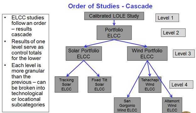
List of Tables
Table 1: Assignment of WECC regions to modeled SERVM zones..............................................................15
Table 2: Load type definitions - consumption, sales, system and net load ................................................18
Table 3: IEPR Forms and Workbooks and Uses...........................................................................................27
Table 4: Economic/Demographic Forecast Error Probabilities ................................................................... 30
Table 5: Baseline Non-Renewables in RESOLVE (MW) ...............................................................................32
Table 6: Baseline Renewables in RESOLVE (MW) .......................................................................................33
Table 7: New Build in RESOLVE for 50% RPS Default Core Case................................................................. 34
Table 8: New Build in RESOLVE for 42 MMT Core Case.............................................................................. 35
Table 9: Resource types modeled in SERVM ..............................................................................................36
Table 10: Generic data inputs common to most resource types (T, F, N, R, C, P, and H)...........................37
Table 11: Generation of Inputs for Child Units from Aggregate Units .......................................................38
Table 12: Inputs related to forced and planned outage hours and statistics for SERVM...........................40
Table 13: Resource Characteristics of Perfect Capacity.............................................................................. 43
Table 14: Variable Operations and Maintenance Costs ............................................................................. 45
Table 15: Input parameters for storage in the SERVM model.................................................................... 46
Table 16: Solar PV Facility Performance Inputs ..........................................................................................51
Table 17: Demand Response Supply-side Modeling Assumptions Summary............................................. 57
Table 18: Demand Response parameters available in SERVM ................................................................... 59
Table 19: Data Sources for Hydropower Inputs..........................................................................................62
Table 20: System Periods ............................................................................................................................66
Table 21: Operating Reserves and Ancillary Service Requirements and Targets ....................................... 67
Table 22: Total Energy Storage Procurement To-Date (IOU Data November 2017) .................................. 71
Table 23: Residual Energy Storage Procurement to Meet D.13-10-040 Targets (MW) .............................71

                                                                        -4-
1 Introduction
The California Public Utilities Commission (CPUC or “Commission,”) staff has prepared this “Draft 2018
Unified Resource Adequacy and Integrated Resource Plan Inputs and Assumptions – Guidance for
Production Cost Modeling and Network Reliability Studies” document (Unified RA/IRP I&A, for short) in
collaboration with staff from the California Energy Commission (CEC) and the California Independent
System Operator (CAISO). A “Final Unified RA/IRP I&A” will be issued once the adopted CEC California
Energy Demand 2018-2030” load forecast has been incorporated into CPUC staff’s production cost
model.
The Unified RA/IRP I&A serves three primary functions:
1. Describe the production cost modeling methodology, inputs, and assumptions that are being
used to inform the CPUC’s Resource Adequacy (RA) proceeding in 2018 (R.17-09-020),
specifically Effective Load Carrying Capability (ELCC) calculations.
2. Describe the production cost modeling methodology, inputs, and assumptions that will be used
to inform the CPUC’s Integrated Resource Plan (IRP) proceeding in 2018 (R.16-02-007),
specifically Loss-of-Load Expectation (LOLE) studies and reserve margin calculations.
3. Describe the inputs and assumptions for use in the network reliability (“power flow”) studies
typical of the CAISO’s 2018-19 Transmission Planning Process (TPP), including the allocation of
load and resource inputs and assumptions to CAISO transmission substations (busbars).
The Unified RA/IRP I&A is “unified” in the sense that it consolidates modeling guidance for the three
primary functions above in a single document and associated sets of data. The production cost
modeling methods and data to support RA and IRP modeling are consolidated in one document because
the two proceedings share a common production cost modeling platform with similar data
requirements. The Unified RA/IRP I&A is also “unified” in the sense of providing for a common and
consistent set of modeling conventions and input data to facilitate comparison and relating of study
results across different planning processes at the CPUC and across different agencies.
The Unified RA/IRP I&A is intended to be used with and be consistent with the “California Energy
Demand 2018-2030” (CED 2017) load forecast that will be adopted with the CEC’s 2017 Integrated
Energy Policy Report (IEPR), expected in early 2018. The Unified RA/IRP I&A is also derived from the
CPUC’s IRP Reference System Plan, adopted by the Commission on February 8, 2018. However, the
CAISO’s TPP schedule requires that the Unified RA/IRP I&A be provided to the CAISO’s Study Plan
development process by mid-February, a deadline ahead of the likely adoption date of the CEC’s 2017
IEPR. The very recent adoption of the IRP Reference System Plan also means the work to translate that
information into the detailed modeling inputs intended for inclusion in this document is in progress.
In order to provide the required input to the CAISO’s TPP and minimize any impact on its schedule, CPUC
staff provides this Draft 2018 Unified RA/IRP I&A document and associated data for use in the CAISO’s
TPP Study Plan development process. Because the Draft 2018 Unified RA/IRP I&A references load data
expected to be final when the 2017 IEPR demand forecast is adopted, it can reasonably provide the
necessary input to the CAISO’s TPP within its required schedule. A Final 2018 Unified RA/IRP I&A will be
-5-provided when staff work to translate both the adopted 2017 IEPR demand forecast and the adopted
IRP Reference System Plan into detailed modeling inputs is complete. The Final version will include any
necessary reconciliation with information provided in the Draft version.
1.1 Background and Roadmap
1
In previous years, the “Assumptions and Scenarios” document was issued annually as a ruling in the
2
CPUC’s Long-Term Procurement Plan (LTPP) proceedings to provide for a common set of data to guide
electric system modeling activities in the LTPP proceeding and the CAISO’s Transmission Planning
Process in that calendar year. The 2016 Order Instituting Rulemaking to Develop an Electricity
Integrated Resource Planning Framework and to Coordinate and Refine Long-Term Procurement
Planning Requirements (R.16-02-007) superseded the LTPP proceedings and is now commonly referred
to as the IRP proceeding. As such, the historical “Assumptions and Scenarios” document is superseded
by this document, the Unified RA/IRP I&A, which is designed for the new IRP process. The detailed data
described by the Unified RA/IRP I&A flows from the IRP Reference System Plan. The Unified RA/IRP I&A
will be updated annually and issued at the beginning of a calendar year. The update planned for the
beginning of 2019 will flow from the IRP Preferred System Plan.
The historical “Assumptions and Scenarios” document was also accompanied by two key Excel
workbook deliverables, the RPS Calculator & Portfolios3 and the Scenario Tool.4 These workbooks are
superseded by new deliverables designed to support the new IRP process. The new deliverables are the
RESOLVE model and a set of workbooks capturing the inputs to the Strategic Energy Risk Valuation
Model (SERVM)5 production cost model being used by CPUC Energy Division staff. The RESOLVE model
was used to develop the IRP Reference System Plan and has been available on the CPUC’s IRP website6
and the workbooks containing SERVM inputs will be provided with the final version of this document
and will be posted on the CPUC Energy Division’s Energy Resource Modeling website.7 The historical
“Assumptions and Scenarios” document was also accompanied by supplemental data and guidance from
the CEC and the three large Investor Owned Utilities to allocate load and resource inputs and
assumptions to CAISO transmission substations. This information will continue to be pointed to or
provided with the new Unified RA/IRP I&A document.
The remainder of this document is comprised of two major sections. First, it describes modeling
conventions and input development for the SERVM model being used to conduct the various types of
production cost modeling studies that are called for in the RA proceeding and the IRP proceeding. This
section of the Unified RA/IRP I&A is sourced from an earlier Energy Division staff document describing
1
The February 2017 version: http://docs.cpuc.ca.gov/PublishedDocs/Efile/G000/M176/K948/176948479.PDF This
document has also been referred to as the Standard Planning Assumptions, or SPA.
2
The previous LTPP proceeding is R.13-12-010.
3
See RPS Calculator v6.2 here: http://www.cpuc.ca.gov/RPS_Calculator/
4
See Scenario Tool 2016 v1.2 here: http://www.cpuc.ca.gov/General.aspx?id=11681
5
Developed by and commercially licensed through Astrape Consulting. http://www.astrape.com/servm/
6
See RESOLVE model here: http://cpuc.ca.gov/irp/proposedrsp/
7
Energy Resource Modeling section data landing page: http://www.cpuc.ca.gov/General.aspx?id=6442451973
-6-the inputs to, and the application of the SERVM model for calculating ELCC values to inform the RA
proceeding in 2017. It is adapted here to inform modeling activities in both the RA proceeding and IRP
proceeding in 2018. The last section of the document describes additional guidance and data required
for the network reliability studies typical of the CAISO’s TPP.
1.1.1 Acronyms
Acronym Definition
1-in-10 1-in-10 year weather peak demand forecast
1-in-2 1-in-2 year weather peak demand forecast
AAEE Additional Achievable Energy Efficiency
AAPV Additional Achievable Photovoltaics (behind-the-meter solar PV)
BTM Behind-the-meter
CAISO California Independent System Operator
CARB California Air Resources Board
CEC California Energy Commission
CED California Energy Demand Forecast
CHP Combined Heat and Power
CPUC California Public Utilities Commission or “Commission”
DCPP Diablo Canyon Power Plant
DR Demand Response
ELCC Effective Load Carrying Capability
EV Electric Vehicle
IEPR Integrated Energy Policy Report
IOU Investor Owned Utility
LCR Local Capacity Requirement
LOLE Loss of Load Expectation
LSE Load Serving Entity
LTPP Long Term Procurement Plan
NQC Net Qualifying Capacity
OTC Once-through-cooling
PG&E Pacific Gas & Electric
POU Publicly Owned Utility
PV Photovoltaic
RPS Renewables Portfolio Standard
SCE Southern California Edison
SDG&E San Diego Gas & Electric
SERVM Strategic Energy Risk Valuation Model
TEPPC Transmission Expansion Planning Policy Committee
TPP Transmission Planning Process
-7-WECC Western Electricity Coordinating Council
2 Production Cost Modeling – Inputs, Assumptions, and Methods
2.1 Scope
This section describes the major assumptions and input sources that the Energy Resource Modeling
(ERM) section in the CPUC’s Energy Division will use when completing Production Cost Modeling (PCM)
to support the Resource Adequacy (RA) proceeding and the Integrated Resource Planning (IRP)
8
proceeding through 2018. This document contains a description of the PCM software the ERM team is
using, the modeling methods, and the inputs and sources. The RA proceeding and the IRP proceeding
will each define the higher-level modeling activities that should be done to support each respective
proceeding. This document only describes the detailed mechanics and data required to conduct the
range of modeling activities that could be requested by the RA and IRP proceedings. The high-level
modeling activities planned for the IRP proceeding in 2018 are described in Attachment B of the IRP
9
Decision D.18-02-018.
This section includes the following key components:
Review of SERVM, software which is being used by Energy Division Staff to conduct LOLE and
ELCC analysis
Primary data sources and assumptions
Interagency coordination
Key modeling processes and order of studies to be undertaken, primarily to perform monthly
LOLE and monthly ELCC studies
Foundational definitions and assumptions for RA and IRP modeling
Key updates and additions since ELCC modeling in early 2017 for the RA proceeding
Gathering and use of weather data for development of synthetic load shapes using weather
normalization and regression analysis
Sources of and use of weather data and weather region definitions to create hourly profiles for
wind and solar production
Data related to conventional (fossil fuel) generators
Burner-tip natural gas price forecasts
Development of data inputs and hourly profiles for hydro generators
Data for demand response and storage resources
Study results will be separately documented and driven by the respective needs of the RA and IRP
proceedings.
8
The previous RA proceeding is R.14-10-010. The current RA proceeding is R.17-09-020. The current IRP
proceeding is R.16-02-007.
9
http://docs.cpuc.ca.gov/SearchRes.aspx?docformat=ALL&DocID=209771632
-8-2.2 Review of SERVM Software
Energy Division staff use SERVM to calculate numerous reliability and cost metrics for a given study year
in light of expected weather, overall economic growth, and unit performance. For each of these factors,
variability and forecasting uncertainties are also taken into account.
As with all probabilistic models, SERVM attempts to simulate the study year many thousands of times
over, with each simulation reflecting a slightly different set of weather, economic, and unit performance
conditions. Iteration conditions are selected probabilistically, based on how likely they are to occur. In
SERVM, a given future study year is modeled by simulating the operation of a fleet of power plants in
that future year to meet hourly electric demand that reflects a wide variety of actual historical weather
patterns. For each of thirty-five possible weather years, six to eight points of load forecast error can be
simulated, creating roughly 210 to 280 scenarios. Each of these scenarios is in turn run with a hundred
or more unit outage draws, creating thousands of iterations for the simulation. Results are expressed as
the probability weighted expected average metrics across the whole range of variability studied. The
results provide a comprehensive distribution of reliability costs, expected unserved energy, and other
reliability metrics. Expected values and confidence intervals can then be calculated based on these
distributions.
2.3 Primary Data Sources and Assumptions
2.3.1 Interagency Coordination and Data Sources
Foundational to the task of coordinating the RA and IRP modeling efforts is coordination between the
key California agencies that cooperatively plan for the future of electric service, including the CEC,
CAISO, and CPUC. Without close integration and coordination, the complicated work described in this
document would be impaired. Chief among the modeling data utilized by Energy Division are the CEC
IEPR that provides electric demand and fuel price forecasts, the CAISO’s datasets which lay out the
generating facilities and transmission topology that operate to provide electricity to customers, and the
CPUC’s IRP and Distribution Resource Plan (DRP) datasets which lay out plans for new investment in
generation and demand side alternatives.
California annual peak and energy demand forecasts including projections of demand-side resources
such as energy efficiency and rooftop solar are sourced from the most recently adopted CEC IEPR
California Energy Demand (CED) forecast. According to agreement between the CAISO, CEC, and the
CPUC, planning processes at each agency will use the Single Forecast Set specified by the most recent
IEPR CED forecast.
Energy Division staff sourced existing CAISO generating unit information from the CAISO MasterFile. In
order to participate in the CAISO energy market and ensure cost effective dispatch of their plants,
generator owners maintain a wide array of information in the MasterFile database. The MasterFile is
used by the CAISO in order to optimize dispatch in light of an array of unit-specific characteristics such as
start-up costs and start-up time, ramp rate, heat rate, and forbidden operating ranges. A number of the
data fields in the MasterFile are confidential, and are accessible to Energy Division staff via an annual
-9-subpoena. Definitions of all the fields in the MasterFile are public and are posted on the CAISO
10
website.
In addition to the CAISO, the Western Electric Coordinating Council (WECC) also compiles a base case
dataset for the WECC and its members to use as a common basis for their modeling. Each Balancing
Authority may have unique access to accurate and confidential data for generators and other market
participants within its footprint, but since the WECC is so interconnected, it is difficult to accurately
model reliability and economic conditions in one Balancing Authority without attention to generators
and loads in the surrounding Balancing Authorities. To facilitate consistent modeling by all Balancing
Authorities in WECC, every two years WECC produces a Common Case dataset containing generic
11
information for all load and supply data across WECC. Produced by a subcommittee of WECC
members called the Transmission Expansion Planning Policy Committee (TEPPC), this dataset is
generated for both the immediate next year and for a year ten years into the future. For modeling
activities during 2018, Energy Division staff imported the TEPPC 2026 Common Case v2.0 into the
SERVM dataset in order to model generating units outside of the CAISO, as well as units in most of the
rest of the Western Interconnect. The peak and energy demand forecasts for regions outside of
California are also sourced from the TEPPC 2026 Common Case.
The TEPPC 2026 Common Case represents the final Common Case dataset that will be produced by
TEPPC. WECC is transitioning to a new organizational model and a new group called the Reliability
Assurance Committee will produce a new dataset called the Anchor Data Set (ADS). We anticipate that
the ADS will take the place of the Common Case and will additionally incorporate modeling inputs for
power flow modeling. Energy Division will transition to ADS data for the next IRP cycle.
The CAISO MasterFile and the WECC TEPPC Common Case dataset each have their advantages and
disadvantages. For generators that supply information to the CAISO MasterFile, there is a larger range of
information available to Energy Division for modeling purposes but some of it is confidential and/or not
directly applicable to production cost modeling.
The WECC TEPPC Common Case dataset, being public data, is often generic and aggregated by class
average. The 2026 TEPPC Common Case has created unit specific heat rate curves and minimum
operating levels based on public data available from the Continuous Emission Monitoring System
database, and this represents a significant improvement in data quality, but there are other areas where
there are challenges to being as precise as possible. For this reason, it is common for particular
Balancing Authorities within the WECC to substitute their own confidential, internal data for the TEPPC
Common Case inputs related to their own specific balancing authority. Energy Division staff will use the
TEPPC 2026 Common Case for regions external to the CAISO balancing area. For regions internal to the
10
MasterFile field definitions can be downloaded from
http://www.caiso.com/Documents/GRDTandIRDTDefinitions.xls. CAISO MasterFile data are confidential, and not
able to be posted; however, it may be possible to aggregate portions of these data for stakeholder review.
11
WECC TEPPC 2026 Common Case v2.0 datasets are available for download here:
https://www.wecc.biz/Reliability/Forms/AllItems.aspx
- 10 -CAISO area, staff will use the generator-specific information obtained via subpoena from the CAISO
MasterFile.
Assumptions for new resources projected to come online by a future study year are sourced from the
IRP proceeding’s Reference System Plan adopted in February 2018 and developed by the RESOLVE
capacity expansion model, or the aggregation of individual LSE Plans to be filed in the IRP proceeding
later in 2018.
All cost data (including generator O&M, startup costs, and fuel handling costs) were adjusted to 2016
dollars using a deflator series developed by the CEC in the IEPR process and which equals approximately
2% inflation, year over year. This is consistent with the convention in the RESOLVE model to report all
costs in 2016 dollars.
Other datasets used by Energy Division staff include the Generator Availability Data System (for
generator forced and scheduled outage statistics), the National Oceanic and Atmospheric
Administration (NOAA) for weather data to generate solar and wind production profiles, the National
Renewable Energy Laboratory (NREL), and data specifically gathered from the utilities. These data and
their use in SERVM will be described in further detail in the sections that follow.
2.3.2 Summary of Model Updates
The SERVM dataset has undergone several important data updates since March 2016. Staff migrated to
the latest version of the 2026 TEPPC Common Case (V2). Staff disaggregated the areas external to
California from 10 areas grouped by state down to 16 areas, grouped by utility service area. For
example, Utah, Colorado, and Wyoming are now WACM, PSCO, and PACE. Staff authorized Astrape
Consulting to restudy and redevelop all solar, wind, and hydro shapes to add actual historical data from
2013 and 2014 to the existing 33 weather years, resulting in two new weather years available for
modeling. Staff also mapped the weather and load shapes to the new utility service areas, and
corrected the mapping of hydroelectric facilities within California. In addition, recent drought
conditions have resulted in lower predicted hydroelectric generation for recent weather years. Hydro,
load, wind, and solar shapes now include 35 years, from 1980 through 2014. There was not sufficient
data available yet to create 2015 shapes.
2.3.3 Key Definitions and Reliability Metrics
Before the development of today’s advanced computing, planners calculated probability of loss-of-load
for the peak hour of each day, and only on weekdays, equating to about 260 data points for a study
year. Today’s computers perform simulations, not simple calculations, and perform simulations of each
hour of the year thousands of times with multiple stochastic variables. Thus a LOLE value of 0.1, which
is a direct translation of the decades old industry “one day in ten years” standard, may warrant
reconsideration in light of the sophisticated hourly models and advanced computing available now.
LOLE and ELCC studies, particularly those done to meet the needs of the IRP and RA proceedings,
require a number of foundational assumptions and modeling conventions in order for the studies to
proceed. Staff made assumptions about what probabilistic reliability standard at which to calibrate the
- 11 -CAISO system for both monthly and annual studies, and the definition of a loss-of-load event. Staff also
performed a convergence analysis to evaluate the optimal number of iterations to run for each case.
In LOLE and ELCC studies for the RA and IRP proceedings, staff will use the following foundational
conventions:
The LOLE reliability target range for calibrating the CAISO system in annual studies will be 0.095
to 0.105 LOLE.
The LOLE reliability target range for calibrating the CAISO system in monthly studies will be 0.02
12
to 0.03 LOLE for each month.
Multiple loss-of-load events occurring within one day shall count as one event for purposes of
counting events towards a reliability target. The loss-of-load event occurs when the frequency
13
response constraint is fully relaxed and when regulation up (1.5% of hourly forecast load) and
spinning reserves (3.0% of hourly forecast load) cannot be maintained, i.e. firm load is assumed
to be curtailed when available capacity is less than 104.5% of load.
2.3.4 General Order of Studies in ELCC Modeling
The scope and sequence of ELCC studies to be done to support the IRP proceeding are defined within
Attachment B of the IRP Decision D.18-02-018.14 The scope and sequence of ELCC studies to support
the RA proceeding are defined in this section. The RA proceeding uses ELCC methods to assign capacity
value to particular resources or sets of resources within a larger electric system. The calibration and
sequence of these studies is critical. The process is illustrated in the following chart:
12
Specifically, the monthly LOLE target was created by first taking the industry standard 0.1 LOLE annual target
and assuming that most of those events map to the four peak months of June through September, or one third of
the year. Assuming a similar target reliability for the rest of the year would mean that total LOLE over the entire
year should have a target of 0.1x3=0.3. Thus, monthly LOLE studies would have a monthly target LOLE of
0.3/12=0.025, i.e. a target range of 0.02 to 0.03.
13
Ancillary services and frequency response requirements are described later in this document in the System
Inputs section 2.10.
14
http://docs.cpuc.ca.gov/SearchRes.aspx?docformat=ALL&DocID=209771632
- 12 -Figure 1: Order of RA ELCC Studies
ELCC studies rely first on LOLE studies, and monthly ELCC studies require monthly LOLE studies. A Level 1
study is to calibrate the LOLE level of the overall electric system to the desired reliability level. Staff will
add or remove electric capacity on a monthly basis in a predetermined order in order to result in a LOLE
that is levelized and within the desired range, i.e. between 0.02 and 0.03.
Once LOLE level is calibrated on a month specific basis, staff will move on to Level 2. Staff will remove
all wind and solar generators from the fleet of generators, in all months, then on a month specific basis,
reinsert Perfect Capacity in increments until LOLE again is between 0.02 and 0.03 in each month.
Level 2 analysis in effect sets a control total meant to represent the total ELCC of the generators in
question. Since there are often interaction and diversity effects between wind and solar generation in
the way they contribute to reliability, this Portfolio ELCC study determines their total ELCC value.
In Level 3 analysts, staff performs individual technology specific ELCC studies, which are studies of a
subset of the Portfolio ELCC studied in Level 2. All wind or all solar generators are removed from the
fleet and Perfect Capacity is added back until LOLE is gain between 0.02 and 0.03 on a month specific
basis. When the ELCC of wind and solar individually are determined, they are totaled and compared to
the Portfolio ELCC results from Level 2. Technology specific ELCC values are adjusted either up or down
so that their total is equal to the Portfolio ELCC value.
When each technology specific ELCC is determined, they become control totals for subsequent Level 4
ELCC analysis. For example, all tracking solar would then be removed, and Perfect Capacity would be
added to return the system to LOLE in the desired range. Then the same with fixed tilt solar, and the
- 13 -resulting ELCC values of fixed and tracking solar would be totaled and compared to the solar technology
ELCC values from Level 3 to see if they would be adjusted upwards or downwards to arrive at their
individual ELCC values.
ELCC values are either expressed as MW equivalent of perfect capacity to a MW total of other
generation, or as a percentage. The percentage ELCC represents the ratio of MWs of Perfect Capacity to
MWs of generation removed. The ELCC percentage factor is applied to the nameplate MW of a
particular generation type to derate its value and demonstrate the amount of “effective capacity” it
provides.
The order of studies above references the steps of removing or adding units to calibrate a system to a
target reliability level. Staff used the following conventions for those steps:
Removal of generation to surface LOLE events in overbuilt systems shall be according to the
15
following order: Conventional thermal generators that have announced their retirement will
be removed first. If LOLE remains below the target level, additional conventional thermal
generation will be removed from CAISO areas ranked by age of the facility. The oldest one will
be removed first, continuing in order of age. No hydro generation or renewable generation will
be removed.
Addition of generation to reduce LOLE events in underbuilt systems shall use perfect capacity as
additions. Perfect capacity is a modeling proxy for generation with no operating constraints, e.g.
always available, starts instantly, infinite ramp rate, no minimum operating level.
Although the calibration step alters the system under study, this is a typical way of performing
ELCC calculations and is not expected to significantly affect the ELCC measurement.
2.4 Weather Data and Regions
Weather is an integral input into probabilistic reliability modeling. It is used both in the development of
synthetic load shapes, which are highly correlated to temperature and humidity, and in the
development of generation profiles for weather-sensitive resources such as wind and solar. In order to
balance the need to model the wide range of weather across the state at any given time and the need to
keep modeling times feasible, a set of representative weather stations are selected and grouped to
create regions that are modeled as homogeneous areas. This section details the weather data utilized,
the sources for this data, the regions modeled, and the process by which these regions were created.
2.4.1 Region Designations
Load, wind, and solar shapes are developed to correspond to regions modeled in SERVM. Staff has
currently organized inputs in SERVM into eight distinct regions within California and sixteen outside of
California based on utility service areas. While most utility service areas are modeled individually, some
are aggregated, as specified in the table below. These regions are utilized throughout SERVM to
associate groups of generation facilities with common weather, load, weather-related generation
15
Note that the order specified here is simply a modeling convention picking one systematic way to remove
capacity for the sole purpose of calibrating a system to a target reliability level in order to perform ELCC
calculations. The choice and order of removing units does not imply the units are likely to retire or should retire.
- 14 -profiles, transmission constraints, and utility service territories. The regions (zones) modeled are listed
in Table 1, below. The regions below do not correspond to transmission-constrained Local Areas, and
are not granular enough for transmission planning. In the future, higher geographic granularity could be
achieved by splitting the regions into smaller areas. However, it is unlikely a production cost model will
ever approach the fidelity required for network reliability (power flow) studies. Such studies are not in
scope for Energy Division staff at this time.
Table 1: Assignment of WECC regions to modeled SERVM zones
California Regions Regions external to California
IID (Imperial Irrigation District) AZPS including HGMA, GRMA, PACW
Balancing Authority Area (BAA) and DEAA
LADWP BAA (includes Burbank and BCHA and AESO PNM and EPE
Glendale)
PG&E TAC16 Area, Bay17 BPA including several smaller Portland General Electric
utilities
18
PG&E TAC Area, Valley CFE PSCO
SCE TAC Area (includes VEA) IPCO SRP
SDG&E TAC Area NEVP and SPPC TEPC
Balancing Authority of Northern NWMT with GWA and WAUW WACM
California (labeled SMUD in the
SERVM model)
TID (Turlock Irrigation District) BAA PACE WALC
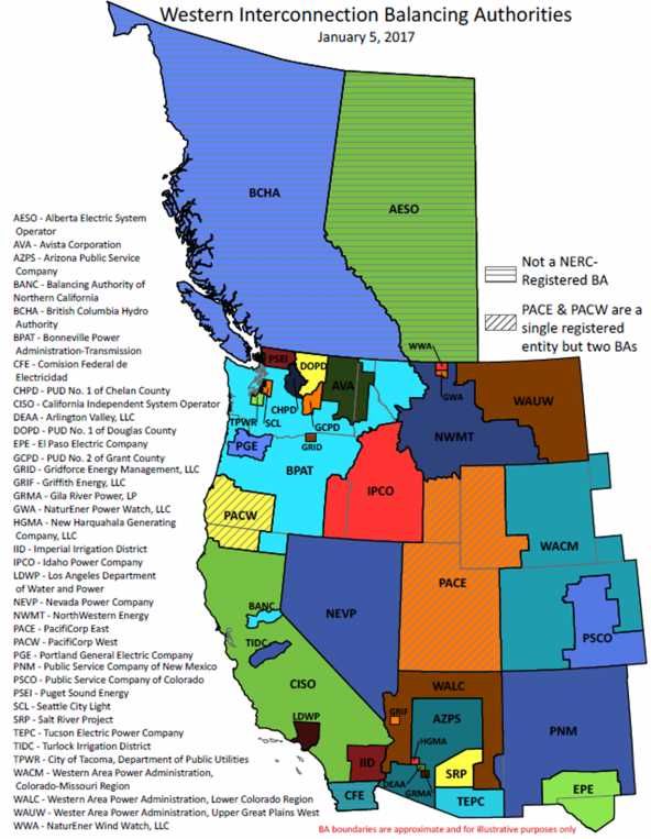
Figure 2 below is an illustrative map of Western Interconnection Balancing Authorities and is generally
consistent with the region definitions used in SERVM.
16
A transmission access charge (TAC) area is a portion of the CAISO-controlled grid where transmission revenue
requirements are recovered through an access charge.
17
Includes these lines from IEPR demand forecast Form 1.5a: CCSF, NCPA-Greater Bay Area, Other NP15 LSEs-Bay
Area, PG&E Service Area-Greater Bay Area, Silicon Valley Power, CDWR-N, CDWR-ZP26
18
Includes these lines from IEPR demand forecast Form 1.5a: NCPA-Non Bay Area, Other NP15 LSEs-Non Bay Area,
PG&E Service Area-Non Bay Area, WAPA, PG&E Service Area-ZP26
- 15 -Figure 2: Balancing Authorities in WECC
Source: WECC website, downloaded January 30, 2018
https://www.wecc.biz/Administrative/Balancing_Authorities_JAN17.pdf
- 16 -2.5 Weather Normalization Process: Development of Hourly Synthetic Load
Profiles
The objective of weather normalization is to create synthetic load profiles that accurately represent the
relationship of hourly customer electricity demand to historical weather patterns, over as wide a range
of historic weather patterns as possible. Of particular importance is the accurate preservation of both
spatial and temporal correlations occurring between historical load and weather patterns. There is also
the need to establish the relationship of recent weather patterns to recent electricity demand. In other
words, relationships between weather and electricity demand are changing as customers use more
efficient lighting and cooling equipment, and as the weather changes due to climate change, so the
relationship between load and weather should be established for a set of recent, representative years.
Our weather normalization is informed by 35 years of historical hourly weather data across the years
1980 through 2014, and is used to develop 35 years of hourly synthetic load shapes for 24 geographical
regions across the western United States. Hourly historical load profiles across the same geographical
regions for the last 5 years of the time series (2010 through 2014) are used to train the model. The
model we use is described in more detail below.
The relationship between weather and electricity demand should focus on the relationship of weather
on a granular locational level to customer electricity consumption, where consumption refers to actual
demand, independent of any self generation. See Table 2 for definitions of the various load types
referred to in this document.
Whereas meter data is available that captures actual energy delivered, or sales, to the customer by the
utility, consumption data is typically not measured directly. However, attempting to model the
relationship between weather and sales, defined as consumption less any self generation, does not
capture a meaningful physical relationship. This is because sales depends, for example, on the number
of solar panels installed on a customer’s roof, which has no relationship to the weather effects
experienced by the electricity customer.
In the absence of customer self generation, consumption and sales are identical, but with increasing
levels of customer self generation, consumption becomes counterfactual. Therefore customer electricity
consumption must be reconstituted from the utility sales values by simulating behind the meter
generation values, based on installed photovoltaic capacity and hourly insolation profiles.
- 17 -Table 2: Load type definitions - consumption, sales, system and net load
Note that in SERVM we are modeling behavior at the system level, and do not explicitly model both sales and
system load. Said another way, we gross up sales to the system level, accounting for losses .
Load Type Relation to Other Terms Rationale Measurement
Consumption Sum of electrical energy Consumption is the With increased self generation, and
used to operate end-use term used in CEC when relying on net energy metering
devices excluding forms to capture to apply cost responsibility to end-
charge/discharge of onsite energy usage. users, consumption becomes
storage counterfactual.
Sales Consumption less BTM Sales is the energy Metered by the utility on a short
onsite generation term to indicate the interval basis if the utility has
including storage net energy delivered deployed interval metering systems
charge/discharge through the meter to for end-users; otherwise could be
the end-use customer estimated using load research
practices
System Sales load plus T&D Standard electricity Generally measured by power plant
losses plus theft and industry term. CEC output and import flows, e.g. a top
unaccounted for defines “hourly down measurement inferring loads
system load” in its rather than a bottom up summation
data collection of individual customer loads
regulations
Net Load System load less system This is the same BAA estimation of system load less
intermittent renewable definition as being measured output of wind and solar
generation used by CAISO supply-side renewables
2.5.1 Data Collection and Scrubbing
Data used in this process includes hourly historical weather data (35 years), and hourly historical load
data (5 years of sales data) along with any hourly self generation or demand response needed to
calculate consumption from sales values. This section describes the data collection and data scrubbing
process required to perform the regression analysis used in the weather normalization process.
- 18 -2.5.1.1 Weather Data
Hourly historical weather data is obtained from the National Climate Data Center (NCDC) for years 1979
through 2014.19,20 Hourly temperature and dew point data are downloaded for nearly 60 weather
stations across the western United States corresponding to the western electrical grid footprint,
including contiguous parts of Canada and Mexico. For California, where we would like our spatial
resolution to be highest, we use over 20 weather stations to inform our model. In several cases, weather
station data needs to be stitched together from geographically adjacent weather stations when a given
station lacks a contiguous history across the full range of years. Note that all hourly weather station data
from the NCDC ISD-Lite dataset are provided in a manner that is corrected for daylight savings, that is,
all hours correspond to standard time in the local time zone.
SERVM uses 24 geographic zones, 8 of which are located in California. Weighted temperature and dew
point values are determined for each of the 24 SERVM zones using the 60 NCDC weather stations. A set
of normalized weighting factors mapping the NCDC weather station data to SERVM zones is developed
for each zone by season. The weighting factors are determined by season from the best fit of a
logarithm of consumption load versus linear temperature model.
The raw hourly weather data profiles as obtained from the NCDC contain missing data segments. We
analyzed the distribution of missing data and found the mode length for missing temperature data is
about 10 days, coincidentally roughly the length of time of a typical employee vacation. It may be that
weather station data is captured by a single employee, so that when they are on vacation, missing data
segments occur. Likewise, dew point data also has missing data segments. We fill in missing
observations in both temperature and dew point data using linear interpolation to ensure complete
hourly coverage across the full 35 year time span.
Additionally, hourly solar insolation, wind speed, and cloud cover data was obtained from the NCDC
dataset and developed for use in calculating self generation and system renewable energy production
for use by the SERVM model.
2.5.1.2 Load Data
Developing hourly consumption data requires collecting metered sales data and reconstituting
consumption by adding back the hourly effects of BTM generation or demand response that was not
metered separately. While some hourly BTM self generation and demand response data21 can be
obtained for some geographic regions within California and used to develop hourly consumption profiles
19
National Climate Data Center (NCDC): https://www1.ncdc.noaa.gov/pub/data/noaa/isd-lite/
20
While the weather normalization spans 1980 through 2014, 1979 is used to remove boundary issues that arise
when calculating lagged temperature and dew point values at the beginning of the time series, as discussed below.
21
The hourly impacts of demand response are difficult to recreate; for areas internal to CAISO, Energy Division
staff issued a data request for the actual hourly impacts from the three IOUs that manage the demand response
programs from the 2010 to 2016 program years. We collected data for the years 2011 through 2016 to ensure
that the trends were reasonable past 2014, but only hourly data for 2011 through 2014 was used for reconstituting
consumption.
- 19 -from sales,22 it is difficult to obtain this information for all types of BTM effects and for all regions inside
or outside of California. For regions outside California where BTM self generation and demand response
profiles are not available, we simply use hourly sales profiles in lieu of hourly consumption profiles.
While this introduces some error into our weather normalization process, we believe the impacts are
minimal because (a) where BTM self generation and demand response is not available outside of
California over the time frame we are modeling, we expect those quantities to be minimal, and (b) we
are most concerned with the behavior of the electric grid within California, so small discrepancies
between consumption and sales outside California should have minimal impact on our results. As BTM
self generation and demand response profiles outside California become available, we will incorporate
them into our analysis.
Hourly sales data for years 2010 through 2014 is obtained from multiple sources. For California regions
within the CAISO footprint, we use hourly CAISO Energy Management System (EMS) sales data.23 For the
remainder of the WECC footprint, we obtain hourly sales data from FERC Form 714. 24 Hourly sales data
for Pacificorp East and West regions needs to be obtained independently, since it is provided as a single
region in Form 714, whereas staff has elected to model them as two separate zones.25 Sales data for
Canadian regions are also obtained independently.26 Loads for all these regions are mapped into the
zones used in SERVM.
All load data used in the weather normalization analysis is corrected for daylight savings time shifts,
resulting in a consistent dataset in standard time in the local time zone. This is an important step that is
required in order to accurately align hourly load profiles with hourly weather profiles. In many cases,
FERC Form 714 data is not corrected for daylight savings. However FERC Form 714 is provided in a 25
hour format that enables the user to unambiguously correct for daylight savings. 27 In contrast, CAISO
EMS data does not appear to consistently and clearly indicate if and when daylight savings is in effect.
Therefore CPUC staff performed a separate daylight savings correction to the CAISO EMS data in order
to consistently align it with the CPUC weather normalization process.
2.5.1.3 Behind-the-Meter Photovoltaic (BTM PV) Data
Since BTM PV generation is not individually metered or consistently accessible to CPUC staff, hourly
historical BTM PV generation is simulated. This requires a tabulation of cumulative BTM PV installed
22
Actual hourly demand response impacts (taken from utility reports of historical demand response events) are
added back into historical load figures to represent historical loads as if the demand response events had not
occurred. Thus, when demand response events are modeled for the study year in SERVM, there is no double
counting of demand response impacts (triggering modeled events on top of or in addition to historical events).
23
CAISO EMS data is proprietary, and is obtained via subpoena
24
Federal Energy Regulatory Commission (FERC) Form 714: https://www.ferc.gov/docs-filing/forms/form-
714/overview.asp
25
Pacificorp data was obtained via subpoena
26
British Columbia (BC) hydro data: http://www.bchydro.com/energy-in-
bc/our_system/transmission/transmission-system/balancing-authority-load-data/historical-transmission-data.html
27
FERC Form 714 instructions for participating Load Serving Entities instruct that a zero load should be placed in
the March skip ahead day to indicate when daylight savings goes into effect, and a 25th hour load should be
provided in the November fall back day when reverting back to standard time. This unambiguously allows for
adjustment to standard time in the local time zone.
- 20 -capacity by month and SERVM region, and the hourly production profile of PV generators by SERVM
region, from January 1, 2010 to December 31, 2014. The source of BTM PV installed MW per month for
areas within the CAISO area is CaliforniaDGStats.ca.gov.28 The source of BTM PV MW for Balancing
Authorities (BAA) and utilities outside of CAISO is Energy Information Administration (EIA) form 861 Net
Metering data.29 We obtained EIA data for 2011-2016 and using the “Utility Level-States” tab, we
filtered it to retain the BAAs within the WECC. We extracted data for the years 2011 through 2016 just
to ensure that the trends were reasonable past 2014, but only hourly data for 2011 through 2014 was
used for the weather normalization work. 2010 data was not available from EIA information, so we had
to assume that the effect could be ignored. As mentioned above, California information was available
from a different source, which had data for the full 2010 to 2014 timeframe so modeling of California
areas should be more accurate.
To detect anomalies in the data, we created filled line charts showing total installed BTM PV MW by BAA
and utility, by year and month for the 6 year period. The EIA Form 861 data consists of total installed
BTM PV MW, so the curves are expected to increase and include some flat sections when BTM PV
installations slow. The charts we created with EIA Form 861 data revealed some dips and steep
increases, indicating incomplete data. For months in which the dips or steep increases were more than 4
MW, we calculated reasonability adjustments. We made adjustments to less than 1% of the data lines,
for nine utilities in five states outside of California. Using the installed MW values by month and SERVM
region with the hourly production profiles for solar generation, we simulated hourly BTM PV effects
which were added back to hourly sales data to reconstitute consumption.
2.5.2 Weather Normalization Model
The weather normalization approach we take is based on the Monash Electricity Forecasting Model, 30
and is consistent with the approach taken by the California Energy Commission’s weather normalization
31
process. In this approach, each hour of the day is modeled separately, and reconstituted at the end of
the process. This allows us to develop different regression relationships between hourly load and the
driver variables (e.g. temperature and dew point) for different hours of the day. For example, during
peak load hours, the relationship between the weather driver variables and consumption is more tightly
constrained than during off peak hours, so we expect a better fit to the regression relationship for these
model hours. Furthermore, the model also separates out the impacts of the average annual load, a
scalar quantity defined by year, from the corresponding normalized hourly load profile shape. This
feature of our approach essentially separates the scalar magnitude from a normalized load shape.
In the production cost modeling (PCM) analyses performed by the CPUC, we rely on the CEC IEPR
forecasts as the basis for the magnitude of the average annual and peak load characterizing load profiles
in the target year. Both average annual and peak load are scalar quantities defined for each target year
28
These data are available for download at https://www.californiadgstats.ca.gov/
29
These data are available for download at https://www.eia.gov/electricity/data/eia861/
30
Monash Electricity Forecasting Model, see: https://robjhyndman.com/papers/MEFMR1.pdf
31
CEC Demand Analysis Working Group, Friday, March 17, 2017, Forecasting Hourly Loads, see:
http://www.dawg.info/sites/default/files/meetings/2.2017%2003-
17%20DAWG%20Long%20Term%20Hourly%20Elec%20Model%20Vaid.pdf
- 21 -in the CEC’s 10 year IEPR forecast. We linearly scale the normalized load profiles generated by our
regression analysis in a manner that preserves the average annual and peak load for each target year
modeled in our PCM (see Section 2.6.3 for more information on the load stretching algorithm). Because
the approach we take separates impacts of the magnitude of the average annual and peak load from the
corresponding normalized load profile, and because we rely directly on the CEC IEPR forecast to
determine average annual and peak load, the weather normalization process we use here is only
concerned with developing a regression relationship between weather and normalized hourly load
profiles, for each geographic region in question.
In our model, denotes the model hour, where ranges from 1 to 24. If t denotes the hour in our time
series data corresponding to the most recent 5 years over which the regression relationship is derived,
then t ranges from 1 to approximately ~ 24 × 365.25 × 5 , where the approximation depends on
where the leap year falls. Given our hourly model, we can write as = [( − 1) 24] + 1.
As mentioned above, the model used to create a relationship between hourly load and the driver
variables separates average annual load from a normalized peak load profile, and for each region can be
32
written as:
∗ ( )
( , )= ( , )+ (1)
Where:
, is the hourly load for model and hour t
∗
, is the normalized load profile
is the average annual load corresponding to year i
We can then use the Monash approach to model the normalized peak load profile as:
∗ ( )+ ( ) + ( )+
( , )= , + (2)
Where:
( ) models the effects of the weighted temperature WT
( ) models the effects of the weighted dew points DP
ℎ ( ) models all calendar effects, including dummy variables for month, day of week, and
holidays
ℎ ( ) models all calendar effects, including dummy variables for month, day of week, and
holidays
ResRate , models the effects of the residential retail rate, which serves to balance energy
consumption across the model regions, in which a relatively higher retail rate should lead to
lower consumption
32
Recall log(ab) = log(a) + log(b)
- 22 -You can also read