Large and increasing methane emissions from eastern Amazonia derived from satellite data, 2010-2018
←
→
Page content transcription
If your browser does not render page correctly, please read the page content below
Atmos. Chem. Phys., 21, 10643–10669, 2021
https://doi.org/10.5194/acp-21-10643-2021
© Author(s) 2021. This work is distributed under
the Creative Commons Attribution 4.0 License.

Large and increasing methane emissions from eastern Amazonia
derived from satellite data, 2010–2018
Chris Wilson1,2 , Martyn P. Chipperfield1,2 , Manuel Gloor3 , Robert J. Parker4,5 , Hartmut Boesch4,5 , Joey McNorton6 ,
Luciana V. Gatti7 , John B. Miller8 , Luana S. Basso7 , and Sarah A. Monks9,a,b
1 National Centre for Earth Observation, University of Leeds, Leeds, UK
2 School of Earth and Environment, University of Leeds, Leeds, UK
3 School of Geography, University of Leeds, Leeds, UK
4 Earth Observation Science, School of Physics and Astronomy, University of Leicester, Leicester, UK
5 National Centre for Earth Observation, University of Leicester, Leicester, UK
6 European Centre for Medium-Range Weather Forecasts, Reading, UK
7 Earth System Science Center (CCST), National Institute for Space Research (INPE), Av. Dos Astronautas,

1758, 12.227-010, São José dos Campos, SP, Brazil
8 Global Monitoring Laboratory, National Oceanic and Atmospheric Administration, Boulder, Colorado, USA
9 independent researcher
a formerly at: CIRES, University of Colorado Boulder, Boulder, CO, USA
b formerly at: Chemical Sciences Division, NOAA, Earth System Research Laboratory, Boulder, CO, USA

Correspondence: Chris Wilson (c.wilson@leeds.ac.uk)

Received: 30 October 2020 – Discussion started: 10 November 2020
Revised: 1 April 2021 – Accepted: 20 April 2021 – Published: 14 July 2021

Abstract. We use a global inverse model, satellite data and     over larger regions than normal within the Amazon basin.
flask measurements to estimate methane (CH4 ) emissions         We compare our posterior CH4 mole fractions, derived from
from South America, Brazil and the basin of the Ama-            posterior fluxes, to independent observations of CH4 mole
zon River for the period 2010–2018. We find that emis-          fraction taken at five lower- to mid-tropospheric vertical pro-
sions from Brazil have risen during this period, most quickly   filing sites over the Amazon and find that our posterior fluxes
in the eastern Amazon basin, and that this is concurrent        outperform prior fluxes at all locations. In particular the large
with increasing surface temperatures in this region. Brazil-    emissions from the eastern Amazon basin are shown to be
ian CH4 emissions rose from 49.8 ± 5.4 Tg yr−1 in 2010–         in good agreement with independent observations made at
2013 to 55.6 ± 5.2 Tg yr−1 in 2014–2017, with the wet sea-      Santarém, a location which has long displayed higher mole
son of December–March having the largest positive trend in      fractions of atmospheric CH4 in contrast with other basin lo-
emissions. Amazon basin emissions grew from 41.7 ± 5.3 to       cations. We show that a bottom-up wetland flux model can
49.3 ± 5.1 Tg yr−1 during the same period. We derive no sig-    match neither the variation in annual fluxes nor the posi-
nificant trend in regional emissions from fossil fuels during   tive trend in emissions produced by the inversion. Our results
this period. We find that our posterior distribution of emis-   show that the Amazon alone was responsible for 24 ± 18 %
sions within South America is significantly and consistently    of the total global increase in CH4 flux during the study pe-
changed from our prior estimates, with the strongest emis-      riod, and it may contribute further in future due to its sensi-
sion sources being in the far north of the continent and to     tivity to temperature changes.
the south and south-east of the Amazon basin, at the mouth
of the Amazon River and nearby marsh, swamp and man-
grove regions. We derive particularly large emissions dur-
ing the wet season of 2013/14, when flooding was prevalent

Published by Copernicus Publications on behalf of the European Geosciences Union.
10644                                                     C. Wilson et al.: Increasing Amazon methane emissions, 2010–2018

1    Introduction                                                    2. The uncertainty surrounding the distribution and varia-
                                                                        tion of tropospheric OH means that variations, or neg-
Methane (CH4 ), a strong greenhouse gas emitted from a va-              ative trends, in this major atmospheric sink of methane
riety of anthropogenic and natural sources, is second only              might also have played some role in the stabilisation and
to carbon dioxide (CO2 ) in its importance regarding the an-            renewed rise (McNorton et al., 2016; Rigby et al., 2017;
thropogenic radiative forcing contributing to Earth’s climate           Turner et al., 2017; McNorton et al., 2018). However,
change (Myhre et al., 2013). Approximately 90 % of the CH4              others have found no significant trend in OH during this
that is emitted into the atmosphere is eventually destroyed             period (e.g. Naus et al., 2020; Patra et al., 2021) or even
through reaction with the hydroxyl (OH) radical, and most               a trend in the opposing direction (Zhao et al., 2020).
of the remainder is lost to other, smaller sinks, but a net pos-
itive imbalance means that the atmospheric burden of CH4
has been increasing steadily since preindustrial times (e.g.        In general, anthropogenic emissions of CH4 from fossil fu-
Rubino et al., 2019). With an atmospheric lifetime of ap-           els, agriculture and waste are better constrained than natural
proximately 9 years (Prather et al., 2012), CH4 is a poten-         emissions, particularly in bottom-up inventories (Saunois et
tially important species for short-term gains in mitigation of      al., 2020). The majority of natural emissions come from wet-
anthropogenic climate change (Shindell et al., 2012). How-          lands, with smaller contributions from inland freshwaters,
ever, the magnitude of the total global sources and sinks of        oceans, termites, wild animals and geological seeps. There
CH4 is still not well quantified (Saunois et al., 2020). The        are also small but significant emissions from biomass burn-
geographical distribution and sectoral attribution of methane       ing, which are sometimes counted separately from other an-
emissions, and the inter-annual variation of these sources, are     thropogenic emissions despite often being due to agricultural
also uncertain (Saunois et al., 2016; Schaefer, 2019). This         land clearing (van der Werf et al., 2017).
leads to difficulties in assessing potential emission mitigation       Wetlands are the largest single-sector contributors to the
strategies, hampering our ability to meet and assess the cri-       global methane flux (Saunois et al., 2020), and the basin
teria for limiting the global temperature increase put forward      of the Amazon River in South America, covering an area
as part of the Paris climate agreement (Nisbet et al., 2019).       of approximately 6 000 000 km2 (Poulter et al., 2010), is a
   The atmospheric methane burden is now approximately              significant contributor to the global wetland CH4 emission
2.5 times larger than it was in 1750 (Rubino et al., 2019).         budget (Wilson et al., 2016; Bloom et al., 2017). Approx-
The global mean burden stabilised between 2000 and 2006,            imately 60 % of the basin is within the borders of Brazil.
after which it began increasing again (Nisbet et al., 2016).        Wetland regions within Amazonia generally include sea-
Concerningly, the rate of increase of the atmospheric burden        sonal floodplains in the east and swamps, bogs, and marsh
has accelerated since 2014 (Nisbet et al., 2019). This sug-         regions in the west, along with areas of mangroves along
gests that CH4 emissions have been increasing at an accel-          parts of the coast. Throughout the rest of this study, we
erated rate during the past decade, but our understanding of        group all of these distinct ecosystems together as “wetlands”
how emissions are changing is complicated by the following.         for brevity. As well as a number of large wetland sources
                                                                    within South America, there are often significant contribu-
                                                                    tions from fires during warmer, drier years (van der Werf
    1. Attributing a potential emission increase to a particu-      et al., 2017). Recent studies have suggested that there is
       lar region and/or sector is complex, leading to conflict-    also a direct contribution of fluxes entering the atmosphere
       ing hypotheses regarding the changing fluxes (e.g. Nis-      via trees in the Amazon, although there are likely some
       bet et al., 2016; Worden et al., 2017; Monks et al.,         cases of this flux having been already included as part of
       2018; Schaefer, 2019; Lan et al., 2019; Jackson et al.,      the wetland flux in some inventories (Pangala et al., 2017).
       2020). Indeed, whilst rising atmospheric mole fractions      In fact, the contribution of each of these sources of CH4 ,
       of greenhouse gases usually signifies increasing anthro-     along with their regional distribution and variability over
       pogenic influence, the changing isotopic signature of at-    time, is still relatively uncertain. In studies published in the
       mospheric CH4 as the burden rises initially appears to       2000s and early 2010s, estimates of CH4 emissions from the
       indicate that fossil fuel emissions might not be the main    Amazon basin ranged from 4 to 92 Tg(CH4 ) yr−1 (hence-
       driver for the increase (Schaefer et al., 2016; Nisbet et    forth Tg yr−1 , Melack et al., 2004; do Carmo et al., 2006;
       al., 2019; Fujita et al., 2020). Other sectors, including    Miller et al., 2007; Kirschke et al., 2013), but recently es-
       anthropogenic agricultural emissions, could be respon-       timates have converged somewhat, e.g. 31.6–41.1 Tg yr−1
       sible. On the other hand, it has been argued that increas-   (Wilson et al., 2016), 42.7 ± 5.6 Tg yr−1 (including tree flux,
       ing fossil fuel emissions could still be reconciled with     Pangala et al., 2017) and 44.4 ± 4.8 Tg yr−1 (Ringeval et
       the observed isotopic signature, along with increasing       al., 2014). The global wetland total was recently estimated
       biogenic fluxes, if emissions from fires have decreased      to be 148 ± 25 Tg yr−1 from bottom-up estimates and 159–
       during the same period (Worden et al., 2017; Thompson        200 Tg yr−1 from top-down models (Saunois et al., 2020),
       et al., 2018; Howarth, 2019; Chandra et al., 2021).          which implies that if the majority of the emissions from the

Atmos. Chem. Phys., 21, 10643–10669, 2021                                           https://doi.org/10.5194/acp-21-10643-2021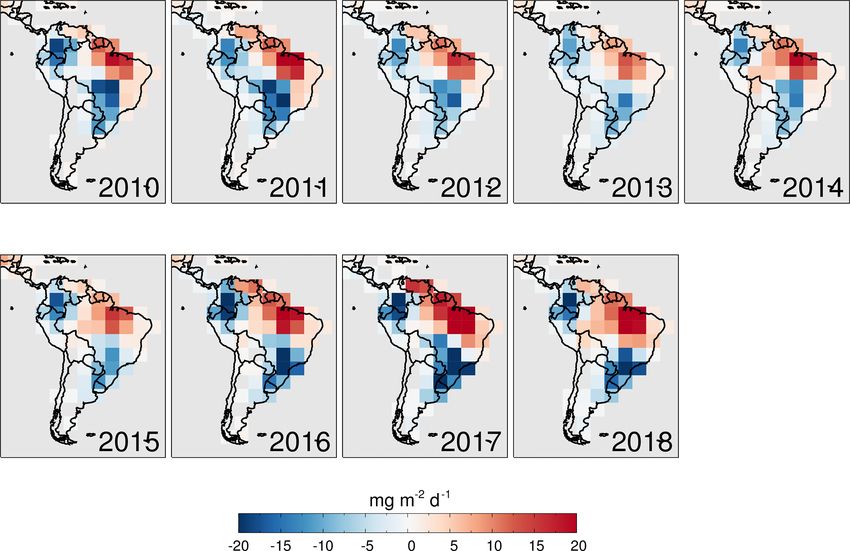
C. Wilson et al.: Increasing Amazon methane emissions, 2010–2018                                                               10645

Amazon are from wetlands, then the region contributes up to
∼ 30 % of the global CH4 wetland flux.
   Many studies have attempted to estimate national CH4
emissions rather than from ecosystems such as the Amazon,
partly as it will likely be easier for countries to put in place
emission reduction protocols on a national basis. Some re-
cent studies have therefore reported emission totals for the
country of Brazil. The synthesis of Saunois et al. (2020)
used a suite of top-down models to find a wide range of
47.3–78.2 Tg yr−1 total emissions from all sources within
Brazil during the period 2008–2017. Natural sources made
up 26.9–53.8 Tg yr−1 of this total. Janardanan et al. (2020)
used a global inversion to constrain total Brazilian emis-
sions to 56.2 ± 10 Tg yr−1 in the period 2011–2017. How-
ever, Tunnicliffe et al. (2020) used a high-resolution regional
inversion to find much smaller emissions from the country,
calculating total Brazilian emissions of 33.6 ± 3.6 Tg yr−1 ,
                                                                   Figure 1. Locations of NOAA surface sites from which flask-based
with wetlands making up 13.0 ± 1.9 Tg yr−1 of this total. The
                                                                   measurements of CH4 are assimilated (blue squares), along with
relatively large range of estimates produced by these studies,     locations and values of GOSAT XCH4 retrievals for August 2017
some of which make use of the same observational datasets,         (circles). Inset shows locations of flight-based observations of CH4
is indicative of the difficulties inherent in using top-down       within the Amazon basin (green triangles).
methods to assess surface emissions of CH4 from within the
poorly monitored continent of South America. However, in
order to best understand the global methane budget and its         2     Methods
sources, it is still vital that the significant contribution of
South American emissions is evaluated and attributed.              2.1     Observations
   In order to best unite these estimates, regular observation
of atmospheric methane over South America is necessary.            We assimilate both in situ flask observations and GOSAT re-
The Thermal And Near infrared Sensor for carbon Observa-           trievals of CH4 into the inverse model. We also use, but do
tion Fourier Transform Spectrometer (TANSO-FTS) instru-            not assimilate, a set of observations made as part of regular
ment on the Greenhouse Gases Observing Satellite (GOSAT;           flask-based aircraft monitoring campaign within the Amazon
Kuze et al., 2009) is particularly advantageous, as it is sen-     basin since 2010 for validation of our results.
sitive far down into the troposphere and has been provid-
                                                                   2.1.1    Surface flask observations
ing regular global coverage of atmospheric CH4 continu-
ously since April 2009 (Parker et al., 2020a). This decade         We assimilate global long-term surface data of CH4 provided
of uninterrupted global coverage allows for understanding of       by the National Oceanic and Atmospheric Administration’s
methane variations over a much longer period than many of          Global Monitoring Laboratory (NOAA GML, Table A1 in
the other available datasets, particularly in the tropics.         the Appendix). We use data from 56 background monitoring
   In this paper we use CH4 observations from GOSAT along          sites, the locations of which are shown in Fig. 1. Whole air
with flask measurements both from within and outside the           samples in flasks are collected weekly to biweekly (every 2
Amazon basin to provide an almost complete 10-year record          weeks) at each site, and CH4 is measured using gas chro-
of methane emissions from South America, beginning in              matography with a flame ionisation detection method (Dlu-
2009. We use the TOMCAT chemical transport model and               gokencky et al., 2018). Data from these sites are assimilated
its inverse model, INVICAT, to quantify emissions and their        in order to constrain the background variations in CH4 mole
uncertainties during this decade. Ours aims are to (1) as-         fractions at the Earth’s surface. The observations made at
sess the geographical distribution of South American CH4           these locations have high accuracy but are generally located
emissions, with focus on the country of Brazil and the Ama-        in regions that are not near significant sources of CH4 . There
zon basin ecosystem; (2) examine how these emissions have          is a relative lack of regular observation in tropical regions,
changed during the previous decade; and (3) investigate why        where CH4 emissions are significant and uncertain. These
any changes to natural emissions might have occurred. We           observations can therefore provide accurate values for back-
describe the observations used and the modelling methodol-         ground CH4 mixing ratios but are not usually able to pro-
ogy in Sect. 2. We show our results and discuss our findings       vide accurate regional CH4 distributions in those areas that
in Sects. 3 and 4, respectively.                                   require the most constraint.

https://doi.org/10.5194/acp-21-10643-2021                                          Atmos. Chem. Phys., 21, 10643–10669, 2021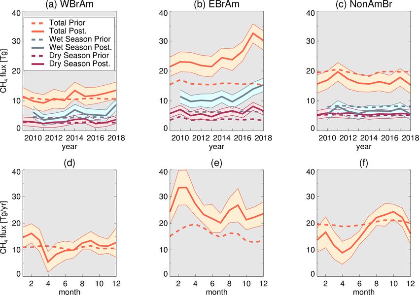
10646                                                   C. Wilson et al.: Increasing Amazon methane emissions, 2010–2018

2.1.2   GOSAT observations                                        to the GOSAT XCH4 . We applied the averaging kernels to
                                                                  the three-dimensional (3-D) CH4 output from the flask data
We also assimilate column-averaged dry-air mole fractions         inversion and calculated the model–observation zonal mean
of CH4 (XCH4 ) from the University of Leicester Proxy re-         bias B(ϕ), in parts per billion (ppb), as a function of latitude
trieval scheme v7.2 for GOSAT (Parker et al., 2011, 2020a).       (ϕ), over this period:
This dataset has been used in the past in forward modelling
studies to assess wetland CH4 emissions using the TOM-            B (ϕ) = 0.0016ϕ 2 − 0.1ϕ + 4.4,                             (1)
CAT model (Parker et al., 2018, 2020b). The GOSAT Proxy           where ϕ is equal to the latitude of the observation in de-
scheme uses the ratio of the retrieved XCO2 and XCH4 , to-        grees north (see Fig. A1). Positive values of B(ϕ) indicate
gether with model-based estimates of XCO2 , in order to re-       positive observation bias relative to the model. Including a
duce the effects of atmospheric scattering and improve cov-       function that is constant along the longitudinal and tempo-
erage of XCH4 retrievals. This is particularly true in tropi-     ral axes means that all information content from the satellite
cal land regions where the prevalence of cloudy pixels of-        data along these axes is preserved, but this method reduces
ten restricts the successful direct retrieval of XCH4 . GOSAT     conflict between assimilation of the satellite and flask obser-
XCH4 retrievals have been used previously in a number of          vations. Similar methods have been used before, for exam-
forward and inverse modelling studies (Fraser et al., 2013;       ple in Bergamaschi et al. (2009). Across the tropics (30◦ S–
McNorton et al., 2016; Feng et al., 2017; Miller et al., 2019).   30◦ N), the derived bias varies between 2.8 and 8.8 ppb. Fur-
The observations are regularly validated against independent      ther south, the bias reaches values up to 13.4 ppb. In our anal-
data, including CH4 observations made as part of the To-          ysis we add the estimated bias value to the simulated XCH4
tal Carbon Column Observing Network (TCCON, Wunch et              values in the inversion after the averaging kernels are applied.
al., 2011), although none of the measurement sites included
as part of this network are located within the Amazon re-         2.1.3   Amazonian aircraft profiles
gion. Webb et al. (2016) compared GOSAT XCH4 to verti-
cal profiles of flask-based measurements of CH4 taken at a        We used independent in situ observations of CH4 mole frac-
number of sites within the Amazon basin (described here in        tion made within the basin to validate our inversion results.
Sect. 2.1.3) and found that biases between the satellite re-      Since 2010, aircraft-borne flask air observations of a num-
trievals and the flask observations were not significantly dif-   ber of species, including CH4 , CO2 and carbon monoxide
ferent from zero.                                                 (CO), have been made at five locations within the Amazon
   Before assimilation, GOSAT-retrieved and a priori XCH4         basin (shown in Fig. 1, inset) by researchers at the Insti-
were averaged onto the model grid. Both sun-glint obser-          tuto de Pesquisas Energéticas e Nucleares (IPEN) in Sao
vations over the oceans and nadir observations over land          Paulo, Brazil, until 2014 and at the National Institute for
were included in the inversion. All XCH4 values measured          Space Research (INPE) São José dos Campos, Brazil (2015–
by the satellite during one model time step in the same grid      present). The sites are located at Santarém (SAN, 2.9◦ S,
cell were averaged using a weighted mean according to their       55.0◦ W), Tabatinga (TAB, 6.0◦ S, 69.7◦ W), Alta Floresta
uncertainties. The largest number of observations combined        (ALF, 8.9◦ S, 56.7◦ W), Rio Branco (RBA, 9.3◦ S, 67.9◦ W)
into a single value was 32, and the mean number was 4.7           and Tefé (TEF, 3.6◦ S, 66.5◦ W). Measurements were only
over land and 6.0 over oceans. Within the Amazon basin,           ever made concurrently at four locations, as the measure-
the mean number of observations combined was 3.8. Fig-            ments at Tefé were started in 2013, to replace those made
ure 1 shows an example monthly distribution of observations       at Tabatinga up to 2012. We therefore combine observa-
used in the inversion. For accurate comparison between the        tions made at these locations and refer to them as TAB/TEF
retrieved XCH4 and those simulated by the model, GOSAT            throughout this paper. Both sites are located in the north-
averaging kernels falling in the same model grid cell and time    west of the Amazon basin and sample similar incoming air
step were averaged, similarly to the XCH4 , and applied to the    masses. Flights are undertaken at approximately biweekly
model vertical profile. Using a single model profile in each      (every 2 weeks) intervals above each site up to an altitude
grid cell and model time step allows the use of averaging ker-    of ∼ 4.4 km, and 0.7 L flasks were filled every 300–500 m to
nels that have been averaged in this way without introducing      produce vertical profiles. All measurements were taken be-
a bias, due to the distributive property of matrix multiplica-    tween 12:00 and 13:00 local time, when the boundary layer is
tion. Retrievals where the model and satellite surface pres-      fully developed. The flasks were analysed for CH4 mole frac-
sure differed by more than 50 hPa were rejected.                  tions at the high-precision gas analytics laboratory at IPEN
   Due to a range of potential error sources in both the at-      and INPE, following the NOAA GML approach, including
mospheric transport model and the GOSAT retrievals, there         rigorous calibration to the World Meteorological Organiza-
is a persistent bias between them, which varies with lati-        tion (WMO) CH4 mole fraction scale. The measurement lo-
tude. We quantified this bias by comparing the results of a       cations were chosen in order to sample the dominant tropo-
previous inversion, in which only the surface flask observa-      spheric airstream across the basin. These observations were
tions had been assimilated for the full 2009–2018 period,         not assimilated in the inversion. For more information about

Atmos. Chem. Phys., 21, 10643–10669, 2021                                         https://doi.org/10.5194/acp-21-10643-2021
C. Wilson et al.: Increasing Amazon methane emissions, 2010–2018                                                            10647

these measurements, see Gatti et al. (2014) and Basso et              For the assimilated surface observations, the model out-
al. (2016).                                                        put was linearly interpolated to the correct longitude, latitude
                                                                   and altitude at the nearest model time step. For the averaged
2.2     Model set-up                                               GOSAT observations, the model mole fractions were inter-
                                                                   polated to the correct longitude and latitude at the nearest
                                                                   time step, before the GOSAT averaging kernels were applied
2.2.1    Inverse model set-up                                      to the model output to give an XCH4 value comparable with
                                                                   GOSAT. GOSAT observations are given an uncorrelated un-
The TOMCAT model is a global 3-D Eulerian offline chem-            certainty equal to 2.5 times the supplied retrieval error, which
ical transport model (CTM) (Chipperfield, 2006; Monks et           ranged from 3.5 to 25.8 ppb, in order to account for repre-
al., 2017). It has been used in a number of previous stud-         sentation error and observation correlations removed by the
ies of atmospheric composition and transport (e.g. Wilson et       averaging of the retrievals, as in Chevallier (2007). This in-
al., 2016; McNorton et al., 2016; Parker et al., 2018). We         flation value was based on the mean number of observations
use the INVICAT inversion framework (Wilson et al., 2014),         combined in each grid cell. In short sensitivity tests, the mag-
which is based on the TOMCAT model and its adjoint. IN-            nitude of posterior emissions was not sensitive to this infla-
VICAT uses a variational scheme based on 4D-Var methods            tion factor once it was larger than 2, although the posterior
used in Numerical Weather Prediction (NWP) and has been            error estimate was affected. This choice gave a mean GOSAT
used in the past to constrain emissions of species including       XCH4 uncertainty value of 24.4 ppb. NOAA observations are
CO2 , ethane (C2 H6 ) and nitrous oxide (N2 O) (Gloor et al.,      given uncorrelated errors of 3 ppb plus representation error.
2018; Monks et al., 2018; Thompson et al., 2019; Tian et           For these observations, representation error was estimated as
al., 2020). The inverse method employed by INVICAT is de-          the mean difference across the eight grid cells surrounding
scribed in depth in these previous references. In brief, the       the cell containing the observation location.
method aims to minimise, in a least-squares sense, the value          Prior emissions are given grid cell uncertainties of 250 %
of a cost function. The cost function is an error-weighted sum     of the prior flux value but also included spatial and tempo-
of the model–observation mismatch, plus error-weighted de-         ral correlations. Although inversions such as this do not di-
partures from the a priori flux estimate.                          rectly allow for sectorial analysis of emissions, we use the
   The inversion input is in the form of an a priori mean flux     off-diagonal values of the prior covariance matrix to pro-
value for each grid cell along with an error covariance ma-        vide some information of this nature. Similar to Meirink et
trix for these values, and the output is an a posteriori mean      al. (2008), we split our prior and posterior solutions into the
grid cell flux value and error covariance matrix. Mean a pri-      anthropogenic fossil fuel emissions assumed to be strongly
ori and a posteriori atmospheric mole fractions of CH4 are         correlated in time (FF), as well as emissions with strong
also produced. For brevity, throughout the remainder of this       seasonal cycles from natural, agricultural and biomass burn-
text, we will refer to the mean a priori and a posteriori fluxes   ing sources (NAT + AGR + BB) by imposing prior tempo-
as “prior fluxes” and “posterior fluxes”, respectively. Simi-      ral correlations on the FF contributions. FF emissions in
larly, the mean a priori and a posteriori mole fractions will      each grid cell in each month were correlated with emis-
be referred to as prior and posterior mole fractions.              sions from the same grid cell in other months with an ex-
   The forward and adjoint model simulations were carried          ponential correlation function with a timescale of 9.5 months
out at 5.6◦ × 5.6◦ horizontal resolution, with 60 vertical lev-    (equivalent to a consecutive-month correlation of 0.9). Both
els up to 0.1 hPa. The model time step was 30 min. The me-         NAT + AGR + BB and FF sectors had spatial correlations
teorology was taken from the European Centre for Medium-           imposed between grid cells, based on Gaussian covariance
Range Weather Forecasts (ECMWF) ERA-Interim reanaly-               functions with correlation length scales of 500 km. This gives
ses (ERA-I, Dee et al., 2011). The inversions were carried         global uncertainty of approximately 70 Tg yr−1 . The sectors
out for each year separately and each completed 40 min-            which make up the NAT + AGR + BB and FF emissions are
imisation iterations. For each year’s inversion, 40 iterations     explained in Sect. 2.2.2.
were enough for the cost function and its gradient norm to be         We produced estimates for each year’s posterior emis-
judged to have converged (less than 1 % variation through 5        sion covariance error matrix using cost function gradient val-
consecutive iterations). The inversion for each year was ac-       ues from the limited-memory Broyden–Fletcher–Goldfarb–
tually run for 14 months up to the end of February for the         Shanno algorithm (L-BFGS) that we employ to minimise
following year, with the final 2 months being discarded from       the cost function (Nocedal, 1980), based on the method sug-
the results. This was in order to better constrain fluxes dur-     gested by Bousserez et al. (2015). This iterative method esti-
ing the final months of each year. Each inversion therefore        mates the inverse of the Hessian (the second derivative) of the
overlapped with the following one for 2 months but was ini-        cost function and does not include the off-diagonal elements
tialised using 3-D fields provided from the correct date in the    of the posterior covariance matrix, so the posterior errors de-
previous year, so that total CH4 burden was conserved across       scribed in this paper are likely to be lower limits (Bousserez
years.                                                             et al., 2015).

https://doi.org/10.5194/acp-21-10643-2021                                        Atmos. Chem. Phys., 21, 10643–10669, 2021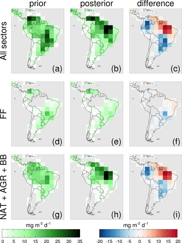
10648                                                    C. Wilson et al.: Increasing Amazon methane emissions, 2010–2018

2.2.2   Prior emissions and chemical sinks of CH4                  varied on a monthly and annual basis and were taken from
                                                                   a previous full chemistry simulation from TOMCAT (Monks
Prior emissions were taken from a range of widely available        et al., 2017). The total simulated atmospheric CH4 sink due
bottom-up models and inventories. Anthropogenic emissions          to reaction with the OH radical in 2009 was 494.5 Tg, whilst
were originally taken from the EDGAR v4.2 FT 2010 inven-           the annual stratospheric CH4 sink due to O(1 D) and Cl was
tory (Olivier et al., 2012) and scaled as in McNorton et al.       19.5 Tg. CH4 loss in the troposphere through reaction with
(2018) to apply an increasing global linear trend for the pe-      Cl was not included in these simulations.
riod after 2012. Biomass burning emissions were taken from
GFEDv4.2 (van der Werf et al., 2017). The JULES model              2.2.3    Bottom-up model
(Clark et al., 2011) was used to provide wetland fluxes, in a
configuration described in McNorton et al. (2016), using four      We also use a simple bottom-up (B-U) model to estimate
separate carbon pools to drive methanogenesis. Rice emis-          wetland CH4 emissions from meteorological and ecological
sions were taken from Yan et al. (2009) and are scaled by          input data, so that we can investigate the causes of variations
a factor of 0.75 as in Patra et al. (2011). Remaining small        in CH4 emissions derived in the inversion. The B-U model,
natural sources (termites, geological and oceanic emissions)       which is based on observed or modelled estimates of wet-
were included as in Wilson et al. (2016). Sectoral emis-           land fraction, heterotrophic respiration of carbon and surface
sion maps are shown in Fig. A2, whilst prior totals for each       temperature, is described fully in Appendix B. The model
source type within South American regions are shown in             uses measurements of gravity anomalies made on the twin
Table 1. The prior global flux of CH4 to the atmosphere            Gravity Recovery and Climate Experiment (GRACE) satel-
rises from 549.5 Tg yr−1 in 2009 to 564.0 Tg yr−1 in 2017.         lite mission as a proxy for variations in wetland fraction. The
The surface soil sink due to methanotrophs was from the            equation that our B-U model is based on is commonly used in
Soil Methanotrophy Model (MeMo, Murguia-Flores et al.,             other studies that estimate wetland fluxes of CH4 (e.g. Clark
2018), repeating the 2009 flux every year, with a value of         et al., 2011; Melton et al., 2013; Bloom et al., 2017), but our
33.9 Tg yr−1 . Landfill and fossil fuel emissions had tempo-       application of the driving climate variables is fairly simple
ral correlations imposed in the prior uncertainty matrix and       relative to these previous works. This method is sufficient
made up the FF category, whilst the remaining emissions            for this work as the purpose of the B-U model is to investi-
(NAT + AGR + BB) had no prior temporal correlations                gate the possibility of reproducing the inversion results, and
imposed. Atmospheric OH fields, based on those provided            if they can be reproduced, to learn how and why the CH4
within the TransCom CH4 study (Patra et al., 2011), were           wetland emissions change according to the input variables. If
taken from Spivakovsky et al. (2000) and scaled downwards          the inversion results are not reproduced using the B-U wet-
by 8 % in accordance with Huijnen et al. (2010). The OH            land model, it could indicate that other sectors played a role
fields used here have previously been shown to capture ob-         in any observed variation.
served atmospheric lifetimes for CH4 and methyl chloroform
(CH3 CCl3 ) in TOMCAT to within the observed uncertainty,          3     Results
although simulations of sulfur hexafluoride (SF6 ) and other
species show that the interhemispheric gradient in TOM-            3.1     Average distribution of emissions
CAT is slightly large compared to observations but within
the bounds of other transport models (Patra et al., 2011; Wil-     Average GOSAT XCH4 values over South America since
son et al., 2014). The OH fields vary from month to month          2009 show that XCH4 column mole fractions were largest
but do not vary between years. Montzka et al. (2011), Naus et      over the west of the continent, particularly in the north-
al. (2020) and Patra et al. (2021) suggested that variability in   west (Fig. 2). Using the prior flux distribution in TOMCAT
annual OH mole fractions is small, but other recent research       leads the model to underestimate XCH4 in the north-east and
has suggested the possibility of a declining trend in OH since     far north of the continent and in the outflow into the At-
2004 (Rigby et al., 2017; Turner et al., 2017), although this      lantic Ocean. Simulated XCH4 is overestimated to the south
trend had a high level of uncertainty. Other studies have          and west of the continent. After assimilation, the largest
found that the El Niño–Southern Oscillation (ENSO) has had         model biases are removed, although there is a small posi-
a significant impact on OH variability in the troposphere in       tive bias in the interior of the continent, usually smaller than
recent decades (e.g. Rowlinson et al., 2019; Anderson et al.,      5 ppb. The posterior (prior) mean model–satellite mismatch,
2020; Zhao et al., 2020), and potentially an increasing trend      weighted by the observation uncertainty, is 0.2 (−24.1) ppb
in tropospheric OH during 1980–2010 (Zhao et al., 2020).           globally, −5.4 (−40.0) ppb within South America and −4.1
A trend in OH, or any year-to-year variability, was not in-        (−66.5) ppb within the Amazon basin. The posterior resid-
cluded in our analysis, which will inform our conclusions,         uals show no significant trend or seasonality within South
but for now we do not have enough evidence to include any          America or within the basin (Fig. A3).
potential variations. Stratospheric loss fields due to reactions      Figure 3 shows the 2009–2018 mean prior and posterior
with atomic chlorine (Cl) and excited oxygen atoms (O(1 D))        emission distributions of CH4 emissions in South America.

Atmos. Chem. Phys., 21, 10643–10669, 2021                                           https://doi.org/10.5194/acp-21-10643-2021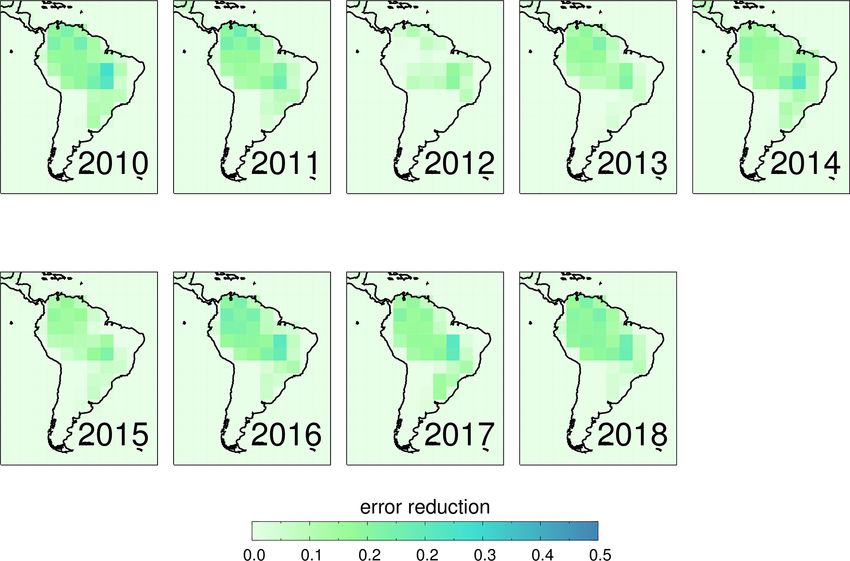
C. Wilson et al.: Increasing Amazon methane emissions, 2010–2018 10649
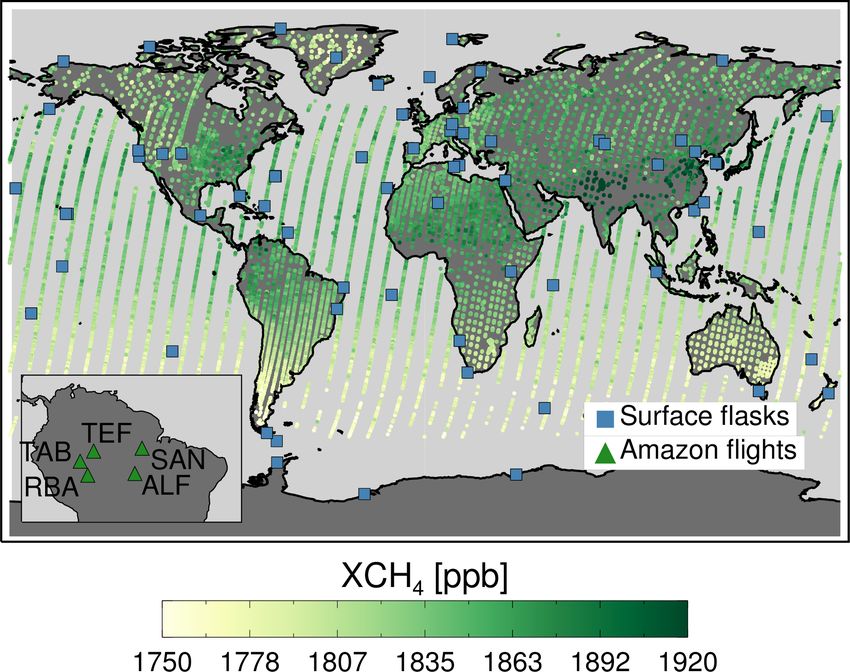
Figure 2. (a) Mean GOSAT XCH4 over South America and surrounding area for 2009–2018. Observations have been averaged onto the
TOMCAT model grid as described in the text. Also shown is the mean difference between the model and satellite XCH4 using (b) the prior
emissions and (c) the posterior emissions for the same period.
We display the mean over this entire period in order to show
the consistent, long-term emission distribution. Whilst pos-
terior uncertainty in particular grid cells can still be fairly
large (Fig. A4), regional changes are much less uncertain.
Posterior South American emissions are significantly redis-
tributed compared to the prior distribution due to changes
in the NAT + AGR + BB emission sectors. Whilst the prior
emissions are fairly homogeneous across much of the Brazil-
ian Amazon, the posterior emissions are largest to the north-
east of the continent and are reduced in the south and the
north-west. Emission rates in the far north of the continent,
potentially related to seasonal flooding in the basin of the
Orinoco river in Venezuela, are also high in the posterior re-
sults.
The most significant feature of the posterior distribution
is a region of high emission rates near the coastal basins
around the mouth of the Amazon River itself (Fig. 3). There
are large emissions from the region around the north-eastern
states of Para, Maranhão and Tocantins. These areas contain
the basins of many of the larger Amazon tributaries and a
high density of wetland sources such as marshes, swamps
and mangroves, according to the Sustainable Wetlands Adap-
tation and Mitigation Program (SWAMP) data from the Cen-
ter for International Forestry Research (CIFOR) (Gumbricht
et al., 2017). The prior flux distribution also highlights agri-
cultural sources near this region in the EDGAR inventory
(Fig. A2).
However, in our posterior results, the western Amazon and
the Pantanal region in the south of Brazil do not display high
emissions. Although the coarse resolution of the model grid
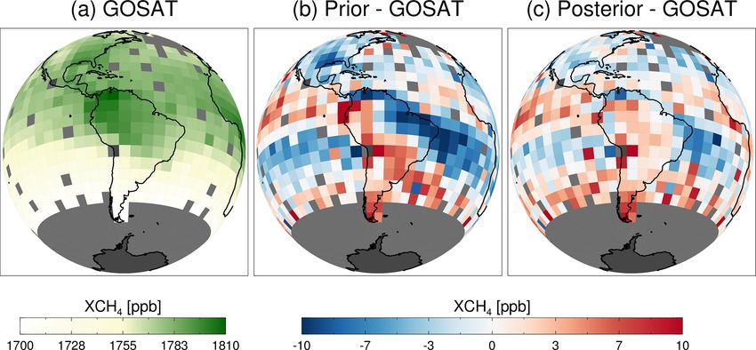
Figure 3. Prior, posterior and (prior–posterior) mean gridded to- boxes masks the signal from the relatively small Pantanal re-
tal South American CH4 emissions (mg m−2 d−1 ) for the period gion in the prior emissions to some extent, it is still surprising
2009–2018 (a–c), and similar but for fossil fuel sources (d–f) and
that the posterior emissions have small methane fluxes from
natural/agricultural/biomass burning sources (g–i) only.
the southern regions of Brazil. As shown in Fig. 2, the model
generally overestimates the XCH4 in southern Brazil com-
pared to GOSAT when using the prior emissions, so it is not
https://doi.org/10.5194/acp-21-10643-2021 Atmos. Chem. Phys., 21, 10643–10669, 2021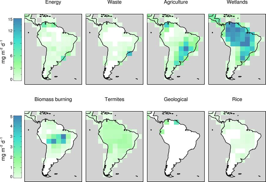
10650                                                       C. Wilson et al.: Increasing Amazon methane emissions, 2010–2018

                                                                      et al., 2020). In Brazil, the mean posterior annual emissions
                                                                      are 49.8 ± 5.4 Tg yr−1 in the period 2009–2013 but rise to
                                                                      55.6 ± 5.2 Tg yr−1 in 2014–2018, with a mean value over the
                                                                      whole period of 52.7 ± 5.3 Tg yr−1 . The uncertainty stated
                                                                      for these figures represents the overall mean annual posterior
                                                                      uncertainty for Brazil derived in the inversion for each 4-year
                                                                      period. We report the mean annual uncertainty as we assume
                                                                      that posterior uncertainty for each year is strongly correlated
                                                                      with that in other years. Reporting the mean value implicitly
                                                                      assumes a correlation of 1 between the years’ uncertainties;
                                                                      in reality the correlation is likely smaller than 1. Our total
                                                                      Brazilian mean flux is within the range found by Saunois
                                                                      et al. (2020) and agrees well with the findings of Janar-
                                                                      danan et al. (2020). There is a significant positive trend over
                                                                      the whole time period (2010–2018) of 1.37 ± 0.69 Tg yr−2
                                                                      (p < 0.05), driven by the NAT + AGR + BB emissions cat-
                                                                      egory, although the distribution actually resembles a step
                                                                      change in 2014.
                                                                         Posterior emissions in Brazil peak in February and
Figure 4. (a) Total annual Brazilian prior and posterior emissions    September (Fig. 4b), representing the wet season and dry
(Tg(CH4 )/yr). Shaded areas show posterior uncertainties as derived   season, most likely due to contributions from the local sea-
in the inversion. (b) Monthly mean prior and posterior Brazilian      sonal cycles of wetland emissions and biomass burning emis-
CH4 emissions (Tg(CH4 )/yr, 2009–2018). Shaded areas show the         sions, depending on the location. The peak monthly emission
standard deviation for each month. (c) Regions of South America       rate of 66.2 ± 8.2 Tg yr−1 is in February, before lower rates
discussed in the text. The hatched area (AmBasin) represents the      of emission during April to July. This February peak corre-
Amazon basin across all countries, whilst the shaded areas show       sponds to a peak in precipitation across the basin (from the
Brazilian and non-Brazilian regions.
                                                                      Global Precipitation Climatology Project (GPCP) v2.3 com-
                                                                      bined precipitation dataset, Adler et al., 2018) but precedes
                                                                      the peak in gravity anomaly – representative of soil water
surprising that emissions from that region were reduced in            depth – captured by the GRACE satellite (Fig. A6). Emis-
the inversion. The low emissions from a region where we ex-           sions in August and September are almost as large as those
pect significant methane release might mean that the model            during the peak of the wet season. Again, almost all of this
transport errors affect comparisons in this region, that the          seasonal variation comes from the NAT + AGR + BB emis-
model–satellite bias included in the inversion (Eq. 1) is in-         sion category.
accurate or that the GOSAT sampling does not cover this re-              Within the entire Amazon region, emissions grew from
gion well (note the relatively small error reduction in this          41.7 ± 5.3 Tg yr−1 in 2010–2013 to 49.3 ± 5.1 Tg yr−1 in
region, Fig. A4). The low emissions in the western Amazon             2014–2017. Emissions are largest in the eastern Brazilian
are also a consistent feature of our results. The FF emissions        Amazon (EBrAm, Fig. 5) and are significantly larger than
do not change significantly in the inversion, although they           suggested by the prior emissions, particularly in the most re-
are slightly decreased towards the south-east of Brazil, close        cent years. The increase in emissions over the period is also
to the large cities of São Paulo and Rio de Janeiro. The over-        largest there, rising from 22.4 ± 3.4 Tg yr−1 in 2010–2013 to
all pattern of the posterior emissions displayed in Fig. 3 is         26.8 ± 3.3 Tg yr−1 in 2014–2017 (trend: 1.06 Tg yr−2 , p <
robust on a year-to-year basis, with the change relative to the       0.01). Emissions also increase from 10.0 ± 2.9 Tg yr−1 to
prior in each individual year displaying very similar patterns        12.3 ± 2.8 Tg yr−1 between these two periods in the western
to the multi-year mean (Fig. A5).                                     Brazilian Amazon (WBrAm). However, in the non-Amazon
                                                                      region of Brazil (NonAmBr), emissions decrease slightly
3.2   Temporal variations of CH4 emissions                            over these years (from 17.5 ± 3.0 to 16.4 ± 2.9 Tg yr−1 ).
                                                                      Trends in WBrAm and NonAmBr are not significant for
The annual total prior emissions in Brazil are nearly constant        p < 0.01. The Amazon regions of Brazil display the two-
over time (Fig. 4), with a mean value of 48.6 ± 14.9 Tg yr−1          peak seasonal cycle of CH4 emissions, although this is much
(uncertainty here from prior error covariance matrix). How-           more pronounced in the east. This is at least partly due to the
ever, the posterior emissions show a positive trend, particu-         significant effect of biomass burning within the arc of defor-
larly from 2013 onwards. Globally, the posterior flux rises           estation in the south-east of the basin that usually occurs dur-
from 566.2 Tg yr−1 in 2009–2013 to 594.0 Tg yr−1 in 2014–             ing these months. Emissions are largest in NonAmBr during
2018 (Table 1), consistent with other studies (e.g. Saunois           the dry season, possibly due to fires or agricultural activity.

Atmos. Chem. Phys., 21, 10643–10669, 2021                                             https://doi.org/10.5194/acp-21-10643-2021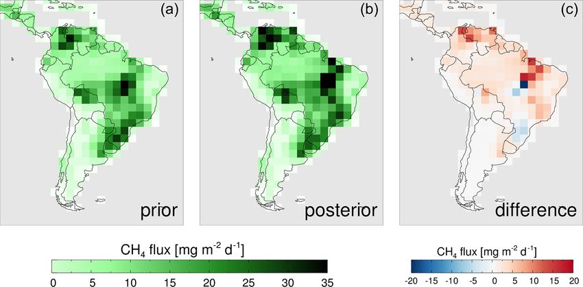
C. Wilson et al.: Increasing Amazon methane emissions, 2010–2018                                                                                           10651

Table 1. Prior and posterior emissions of CH4 for Brazil and other subregions of South America (2010–2017). Units are Tg yr−1 .

                                                 Prior (Tg yr−1 )                                                    Posterior (Tg yr−1 )
                                 2010–2013                             2014–2017                       2010–2013                             2014–2017
                         NAT + AGR + BB             FF    NAT + AGR + BB                  FF    NAT + AGR + BB            FF    NAT + AGR + BB                  FF
 Brazil                       38.9 ± 11.7    10.6 ± 9.2             38.2 ± 11.4    10.6 ± 9.2         39.9 ± 5.3    9.9 ± 0.9               45.7 ± 5.1    9.9 ± 0.9
 South America                59.9 ± 16.4   23.9 ± 16.2             58.5 ± 16.0   23.9 ± 16.2         62.7 ± 7.0   31.6 ± 1.7               68.9 ± 6.7   28.9 ± 1.8
 West Brazilian Amazon         10.1 ± 5.4     0.3 ± 0.5              10.2 ± 5.5     0.3 ± 0.5          9.7 ± 2.9    0.3 ± 0.0               12.0 ± 2.8    0.3 ± 0.0
 East Brazilian Amazon         13.4 ± 7.1     2.7 ± 3.8              12.9 ± 6.7     2.7 ± 3.8         20.0 ± 3.4    2.4 ± 0.3               24.3 ± 3.3    2.5 ± 0.3
 Non-Amazon Brazil             15.4 ± 6.3     7.5 ± 8.4              15.1 ± 6.2     7.5 ± 8.4         10.2 ± 2.9    7.2 ± 0.8                9.3 ± 2.8    7.1 ± 0.9
 Amazon basin                 35.6 ± 12.4     4.1 ± 4.3             35.1 ± 12.2     4.1 ± 4.3         38.2 ± 5.3    3.5 ± 0.3               45.6 ± 5.2    3.7 ± 0.3

Figure 5. (a–c) Total annual (red lines) prior and posterior emissions of CH4 (Tg yr−1 ) in three Brazilian subregions: the western Brazilian
Amazon (WBrAm), the eastern Brazilian Amazon (EBrAm) and non-Amazon Brazil (NonAmBr). Prior and posterior emissions during
the wet season (December–March, grey lines) and the dry season (August–October, maroon lines) are also shown. Shading represents the
posterior uncertainties for each region derived in the inversion. (d–f) Monthly mean prior and posterior emissions for the period 2009–2018
(Tg yr−1 ) for the three subregions. Shading shows the standard deviation of the monthly means.

   We also show total emissions for each subregion dur-                            gions, as seen in version 5.0 of the EDGAR anthropogenic
ing the wet season (December–March) and the dry sea-                               flux inventory in Brazil (Crippa et al., 2020), or some com-
son (August–October). These periods were defined using                             bination of factors. Unfortunately, our results cannot be used
the GPCP precipitation data, as periods when the average                           to say more about which sectors are responsible for the in-
monthly precipitation during 2009–2018 within the basin                            creasing flux.
was more than 7 mm d−1 and less than 3 mm d−1 , respec-
tively. In both WBrAm and EBrAm, the trends for the 2009–                          3.3    Comparison to independent observations
2018 period are largest in the wet season. This suggests that
trends in wetland and floodplain emissions could be respon-                        Observations of CH4 made during flights within the basin
sible for the rising CH4 emissions, in line with reports of                        between 2010 and 2018 were used to independently check
intensifying flood extremes in the area in recent decades                          the performance of the prior and posterior emission distri-
(Barichivich et al., 2018). However, there are other poten-                        butions in the model (Fig. 6, Table 2). For the observations
tial explanations. These include escalating biomass burning                        made at altitudes higher than 3 km, which represents the free
emissions during the wet season (Silva Junior et al., 2019)                        troposphere above the Amazon, the mean bias (MB) between
and an intensification of agricultural emissions in these re-                      model using the posterior emissions and the observations is
                                                                                   significantly reduced at all locations, compared to that pro-

https://doi.org/10.5194/acp-21-10643-2021                                                           Atmos. Chem. Phys., 21, 10643–10669, 2021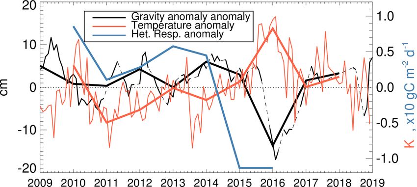
10652                                                      C. Wilson et al.: Increasing Amazon methane emissions, 2010–2018

Figure 6. Histogram plots showing prior (black) and posterior (red) (model–observation) differences at the four Amazon flight locations,
2010–2018. Measurements were taken at Alta Floresta (ALF), Rio Branco (RBA), Santarém (SAN), and Tabatinga and Tefé (TAB/TEF).
Model output has been interpolated to observation locations and altitudes, before both were averaged into monthly means and into altitude
bins of 3 km and above (a–d) and 1.5 km and below (e–h). Dotted vertical lines show the zero line, whilst dashed vertical lines show prior
and posterior mean model–observation bias.

duced when using the prior flux in the model. The correlation          stantially reduces the model–observation difference at SAN.
between the model and the observations also increases at all           The model still underestimates methane mole fractions at
locations when using the posterior flux rather than the prior.         this site even after the improvement, however, which might
The absolute value of the model–observation bias is reduced            be due to bias which remains in the posterior flux estimate,
to below 6 ppb at all sites. However, the posterior model MB           possibly due to the allocated prior uncertainty in this re-
against observations made in the boundary layer, at altitudes          gion being too small, or model representation uncertainty.
below 1.5 km, is higher than the prior model MB at three               The fact that ALF is also located near these significant emis-
sites. At the western sites, RBA and TAB/TEF, the MB in                sions leads to degradation in the model performance within
the model increases by approximately 15 ppb, although the              the boundary layer, which was previously better at ALF than
correlation improves, particularly at TAB/TEF. At ALF, the             at SAN. The capability of assimilation of GOSAT XCH4 to
correlation decreases slightly, and the MB increases by a              improve performance at both of these locations might have
large amount (31 ppb). Finally, at SAN, the performance im-            been reduced due to the relatively coarse model grid. Webb
proves significantly by both measures, with the MB being               et al. (2016) found that comparisons between the flight-based
reduced from −47.8 to −15.2 ppb. There are no significant              observations and a previous version of the GOSAT XCH4
trends (at 95 % level) in the model–aircraft residual biases in        used in this study showed that the GOSAT values were larger
2010–2017, except at TAB/TEF below 1.5 km. This site has               than equivalents estimated using the flight data at ALF but
a posterior residual bias trend of +2.1 ppb/yr, but this may           that the discrepancy was much smaller at SAN. This being
have been caused by the change in the flight location halfway          the case, it is not surprising that the model in which the
through the study period.                                              GOSAT data have been assimilated has difficulties in match-
   The improved performance at SAN is significant, as the              ing the flight observations at both locations at once. Since
high mole fractions of CH4 sampled at this location relative           we assimilated XCH4 from GOSAT, which is mostly rep-
to expectations given its location situated close to the eastern       resentative of the troposphere, it is expected that the model
coast have been previously noted (Miller et al., 2007; Basso           performance is improved at all locations when compared to
et al., 2016; Wilson et al., 2016). The prior model therefore          observations made at the higher altitudes. This also indicates
has a large negative bias at SAN, particularly near the sur-           good model representation of inflow of CH4 to the basin from
face. The posterior distribution of emissions, with a region           elsewhere. However, the fact that the posterior comparisons
of high emission rates to the south and east of the basin, sub-        are generally degraded close to the surface, apart from at

Atmos. Chem. Phys., 21, 10643–10669, 2021                                                https://doi.org/10.5194/acp-21-10643-2021
C. Wilson et al.: Increasing Amazon methane emissions, 2010–2018                                                              10653

                                                                      which rainfall in the south-west of the basin was up to twice
                                                                      as much as usual (Espinoza et al., 2014). This flooded pe-
                                                                      riod did not coincide with a significant ENSO period but was
                                                                      likely caused by warm conditions in the subtropical South
                                                                      Atlantic.
                                                                         Figure 7 also shows the wet season mean anomalies for
                                                                      each year for the surface temperature, gravity anomaly and
                                                                      modelled heterotrophic respiration. Wet season temperatures
                                                                      were high in 2010 and in 2015, 2016 and 2018. The water
                                                                      table was at its highest in 2012, 2014 and 2015. Finally, het-
Figure 7. Anomalies of gravity anomaly (cm, black, left axis),        erotrophic respiration was strongest in 2010, 2013 and 2014
surface temperature (K, red, right axis) and heterotrophic respira-   but very low in 2015 and 2016. There was no heterotrophic
tion (×10 gC m−2 d−1 , blue, right axis) for the period 2009–2018     respiration model data available for 2017, so we used a cli-
within the Amazon basin. Monthly mean anomalies are shown
                                                                      matology value for that year. We felt that this was justified
as thin lines, whilst wet season (December–March) averages are
shown as thick lines. Interpolated values for gravity anomalies are
                                                                      since the temperature and water table depths also had only
shown as dashed lines.                                                very small anomalies during that season. As might be ex-
                                                                      pected, the temperature and gravity anomalies in the wet sea-
                                                                      son were strongly negatively correlated (r = −0.66), due to
SAN, means that the local sources close to these sites might          coincidence of hot and dry conditions.
be overestimated at this model resolution, that there are er-            The temperature trend in the Amazon was positive
rors in the model’s representation of vertical mixing or that         throughout almost the entire basin (Fig. 8a), particularly in
there remains a positive bias in the assimilated retrievals from      the far west and south-east. The trend in the wetland fraction
GOSAT in this region. Generally, however, the temporal vari-          (Fig. 8b) was more heterogeneous, with positive trends in the
ation and MB in the model is much improved after the assim-           west contrasting with strong negative trends across the east
ilation of GOSAT XCH4 .                                               of the basin. Both sets of trends are strongly impacted by the
                                                                      hot, dry conditions in 2015/16.
3.4   Bottom-up model results                                            The geographical distribution of the NAT + AGR + BB
                                                                      wet season CH4 emission trend produced by the inversion
The inversion suggests that CH4 emissions have been signif-           (Fig. 8c) is positive across the north-west and south-east
icantly increasing from eastern Amazon regions throughout             of the basin, with a similar distribution to the temperature
the 2010s, but it is not able to determine the source sectors re-     trends. The positive emission trends in the north-west are col-
sponsible for this rise. The largest increases over time occur        located with an area of increasing wetland fraction. However,
during the wet season (Fig. 5), when wetland emissions dom-           the regions to the east and south with strong positive emission
inate the atmospheric signal, so it is possible that changes to       trends are located where wetland fraction had been decreas-
these emissions led to the increase. Emissions from seasonal          ing as temperatures increased. This suggests that, if wetlands
floodplains and wetlands are sensitive to temperature, precip-        were responsible for increased wet season flux, the methano-
itation (which affects wetland area) and carbon availability in       genesis must have been more sensitive to the increasing tem-
the soil (Bloom et al., 2017), so we examined these factors to        perature than to the decrease in wetland fraction or in het-
see how they varied during the previous decade and whether            erotrophic respiration (not shown).
wetlands could have been responsible for increasing wet sea-             We ran the B-U model multiple times, varying the tem-
son CH4 emission in the basin.                                        perature response and the GRACE anomaly scaling vari-
   The mean surface temperature within the Amazon basin               ables in order to produce a range of likely values for CH4
increased throughout the period 2009–2018 (Fig. 7), while             flux from the basin. We also optimised B-U model param-
there was no significant trend in precipitation (not shown)           eters, as described in Sect. 2.2.3, in order to best repro-
or gravity anomaly. Estimating the trends of these factors is         duce the INVICAT results using the B-U model (Fig. 8d
significantly affected by one anomalously dry and hot period,         and e). The B-U model combines the three driving vari-
running from late 2015 to mid-2016. These record-breaking             ables, but the strong anti-correlation between the tempera-
conditions were caused by the 2015/16 El Niño and were                ture and wetland fractions means that this model does not
largely confined to the east of the basin (Jiménez-Muñoz et           produce strong variations in emissions, since the two tend to
al., 2016). A previous extreme event during this study period,        cancel out. Using the optimised B-U model produces weak
in the dry season of 2010, displayed a similar geographical           positive emission trends in the west of the basin and weak
distribution but was easily surpassed by the scale of the 2016        negative trends elsewhere, giving no significant trend overall
drought (Lewis et al., 2011; Jiménez-Muñoz et al., 2016).             (p = 0.36). The optimised values are included in Appendix
One other event that stands out is the prolonged flooded              B. The standard deviation of the wet season emissions in the
period running through the wet season of 2013/14, during              B-U model is 1.7 Tg yr−1 , compared to 2.4 Tg yr−1 in the

https://doi.org/10.5194/acp-21-10643-2021                                           Atmos. Chem. Phys., 21, 10643–10669, 2021
10654 C. Wilson et al.: Increasing Amazon methane emissions, 2010–2018
Table 2. Prior and posterior bias (ppb) and correlation between TOMCAT and Amazon flight observations (2010–2018). The better value for
bias and correlation for each site and altitude is highlighted in bold.
Prior mean Posterior mean Prior Posterior
bias (ppb) bias (ppb) correlation correlation
ALF, > 3 km −13.7 2.6 0.71 0.75
SAN, > 3 km −19.4 −5.7 0.79 0.88
TAB/TEF, > 3 km −11.1 4.7 0.67 0.81
RBA, > 3 km −9.4 4.6 0.70 0.80
ALF, < 1.5 km 10.2 41.2 0.70 0.67
SAN, < 1.5 km −47.8 −15.2 0.32 0.49
TAB/TEF, < 1.5 km 0.0 15.0 0.48 0.65
RBA, < 1.5 km 5.7 21.4 0.54 0.56
inversion results. The mean posterior error in the inversion This increase between the two periods is very similar
results (2.9 Tg yr−1 ) is relatively large compared to the stan- to that found by Tunnicliffe et al. (2020), although the to-
dard deviation, however, meaning that the B-U values almost tal emissions found in our study are larger than their find-
always remain within the posterior inversion uncertainty. The ing of 33.3 ± 3.7 Tg yr−1 . They removed a model–satellite
exception to this is the wet season of 2014, when the in- bias of 22 ± 8 ppb from the GOSAT observations used in
version results produce larger emissions than in any other their study, which is much larger than our bias of 3–9 ppb
year (20.1 ± 2.7 Tg), and this feature is not reproduced by removed from XCH4 over the Amazon. This treatment of
the B-U model. As discussed, the wet season of 2014 was bias, coupled with differences in model transport, could ex-
subject to extreme precipitation and widespread flooding in plain the different emissions derived. The positive biases in
the basin (Espinoza et al., 2014), and the GRACE gravity our posterior CH4 relative to aircraft observations within
anomalies are large throughout this period (Fig. 7), whilst the boundary layer also suggest that our emissions could
heterotrophic respiration was high and temperatures were be overestimated. However, we note the absence of signif-
relatively cool (although warmer than in 2011 and 2012). De- icant trends in our posterior model minus aircraft residu-
spite these conditions which seem favourable to CH4 emis- als between 2010–2017. Our posterior total emissions agree
sion, the B-U model does not produce emissions significantly well with the findings of Janardanan et al., (2020), who de-
larger than any other year. The discrepancy between the in- rived Brazilian emissions of 56.2 ± 10 Tg yr−1 for the pe-
version and B-U model results is discussed further in Sect. 4. riod 2011–2017, although temporal variation of this value
Figure 8e also shows the wet season emissions within the was not discussed in that study. Yin et al. (2020) did not
basin from the full ensemble (FE) of the WetCHARTs emis- report total emissions but found a rise in Amazonian emis-
sion dataset (Bloom et al., 2017), which use a similar method sions of 4.2 ± 1.2 Tg yr−1 over 2010–2017, along with small
to estimate wetland emissions that used in our B-U model. increases in eastern Brazil. Our estimate of total flux from
These emissions also show a negative trend over the period Amazonia agrees well with that of Pangala et al. (2017), who
2010–2017 (−0.17 Tg yr−1 ), and the variation is again small derived a total of 42.7 ± 5.6 Tg yr−1 for 2010–2013. A group
(0.93 Tg yr−1 standard deviation). They display no signifi- of 22 inverse model experiments presented by Saunois et
cant change in emissions in the wet season of 2013/14. The al. (2020) produced a range of 47.3–78.2 Tg yr−1 for Brazil-
implications of the discrepancy between the inversion and ian emissions between 2008 and 2017, although one of those
the B-U model are discussed in Sect. 4. results used the TOMCAT forward model to represent the
atmospheric transport, so it is not fully independent from
our results. Our findings here are within the range of these
4 Discussion models, albeit towards the lower end. The majority of those
top-down studies used either the same GOSAT and surface
We derive emissions of CH4 in Brazil for the period 2010–
observation data used in our study or some variation of it.
2018 of 52.7 ± 5.3 Tg yr−1 , split into two periods dur-
The fact that the derived emissions using similar observation
ing which mean Brazilian emissions were 49.8 ± 5.4 in
data can vary so much highlights the inherent uncertainties
2010–2013 and 55.6 ± 5.2 in 2014–2017, an increase of
still remaining in top-down studies of CH4 emissions, with
5.8 ± 5.2 Tg yr−1 . This increase was found to be entirely
differences in model transport, chemistry representation, in-
due to the NAT + AGR + BB emissions within the Ama-
version methodology, bias correction and error assumptions
zon region. In Amazonia, emissions grew from 41.7 ± 5.3 to
all contributing to differences in results.
49.3 ± 5.1 Tg yr−1 over the same two periods.
The increase in emissions that we derive from 2014 on-
wards coincides with a faster rate of increase in the observed
Atmos. Chem. Phys., 21, 10643–10669, 2021 https://doi.org/10.5194/acp-21-10643-2021You can also read