Field-scale soil moisture bridges the spatial-scale gap between drought monitoring and agricultural yields - HESS
←
→
Page content transcription
If your browser does not render page correctly, please read the page content below
Hydrol. Earth Syst. Sci., 25, 1827–1847, 2021
https://doi.org/10.5194/hess-25-1827-2021
© Author(s) 2021. This work is distributed under
the Creative Commons Attribution 4.0 License.

Field-scale soil moisture bridges the spatial-scale gap between
drought monitoring and agricultural yields
Noemi Vergopolan1 , Sitian Xiong2 , Lyndon Estes2 , Niko Wanders3 , Nathaniel W. Chaney4 , Eric F. Wood1 ,
Megan Konar5 , Kelly Caylor6,7 , Hylke E. Beck1 , Nicolas Gatti8 , Tom Evans9 , and Justin Sheffield10
1 Civil and Environmental Engineering Department, Princeton University, Princeton, NJ, USA
2 School  of Geography, Clark University, Worcester, MA, USA
3 Department of Physical Geography, Faculty of Geosciences, Utrecht University, Utrecht, the Netherlands
4 Department of Civil and Environmental Engineering, Duke University, Durham, NC, USA
5 Civil and Environmental Engineering Department, University of Illinois at Urbana-Champaign, Urbana, IL, USA
6 Department of Geography, University of California, Santa Barbara, CA, USA
7 Bren School of Environmental Science and Management, University of California, Santa Barbara, CA, USA
8 Department of Agricultural and Consumer Economics, University of Illinois at Urbana-Champaign, Urbana, IL, USA
9 School of Geography, Development and Environment, University of Arizona, Tucson, AZ, USA
10 School of Geography and Environmental Science, University of Southampton, Southampton, UK

Correspondence: Noemi Vergopolan (noemi.v.rocha@gmail.com)

Received: 12 July 2020 – Discussion started: 24 July 2020
Revised: 11 December 2020 – Accepted: 17 February 2021 – Published: 9 April 2021

Abstract. Soil moisture is highly variable in space and time,    ture Organization (FAO). Our results reveal that soil mois-
and deficits (i.e., droughts) play an important role in modu-    ture is the strongest and most reliable predictor of maize
lating crop yields. Limited hydroclimate and yield data, how-    yield, driving its spatial and temporal variability. Soil mois-
ever, hamper drought impact monitoring and assessment at         ture was also a more effective indicator of drought im-
the farm field scale. This study demonstrates the potential of   pacts on crops than precipitation, soil and air temperatures,
using field-scale soil moisture simulations to support high-     and remotely sensed normalized difference vegetation index
resolution agricultural yield prediction and drought monitor-    (NDVI)-based drought indices. This study demonstrates how
ing at the smallholder farm field scale. We present a mul-       field-scale modeling can help bridge the spatial-scale gap be-
tiscale modeling approach that combines HydroBlocks – a          tween drought monitoring and agricultural impacts.
physically based hyper-resolution land surface model (LSM)
– with machine learning. We used HydroBlocks to simu-
late root zone soil moisture and soil temperature in Zam-
bia at 3 h 30 m resolution. These simulations, along with re-    1   Introduction
motely sensed vegetation indices, meteorological data, and
descriptors of the physical landscape (related to topogra-       Droughts can significantly impact crop production, with im-
phy, land cover, and soils) were combined with district-level    plications for food security, particularly in smallholder farm-
maize data to train a random forest (RF) model to predict        ing systems (Kristjanson et al., 2012; Guilpart et al., 2017).
maize yields at district and field scales (250 m). Our model     The impacts of droughts on agricultural production remain
predicted yields with an average testing coefficient of de-      difficult to quantify, especially in developing regions where
termination (R 2 ) of 0.57 and mean absolute error (MAE)         data are generally scarce and crop production can be highly
of 310 kg ha−1 using year-based cross-validation. Our pre-       variable due to substantial climate variability, highly hetero-
dicted maize losses due to the 2015–2016 El Niño drought         geneous landscapes, and variable farming capacities (Lobell,
agreed well with losses reported by the Food and Agricul-        2013; Donaldson and Storeygard, 2016). Challenges in un-
                                                                 derstanding the precise impact of drought on crop yields ex-

Published by Copernicus Publications on behalf of the European Geosciences Union.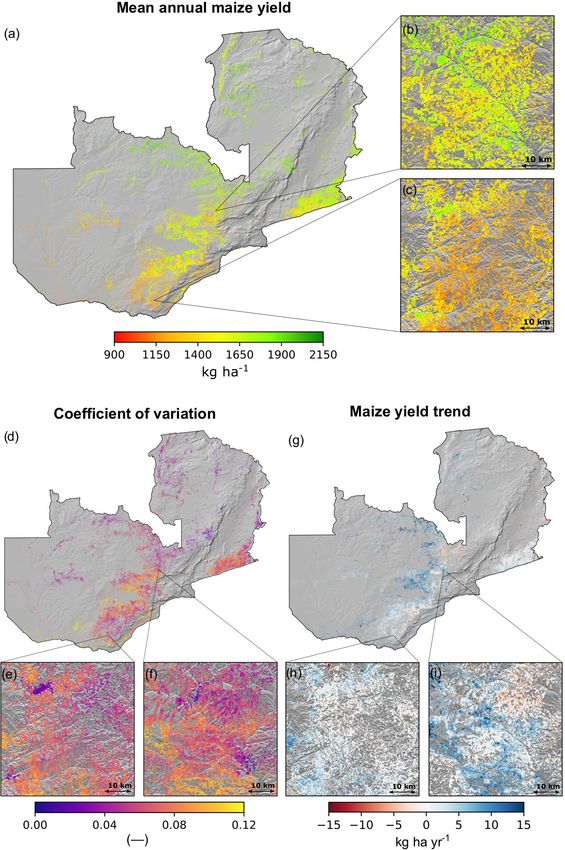
1828              N. Vergopolan et al.: Field-scale soil moisture for agricultural yield prediction and drought monitoring

ist because of the lack of high-quality data and appropri-             To aid drought assessments, data on crop yields are usually
ate drought metrics (Sutanto et al., 2019; Beza et al., 2017;       estimated through self-reported field surveys. However, these
Sadri et al., 2020). These data limitations may lead to pre-        are time-consuming, expensive, and often suffer from sam-
dictions of yields, drought impacts, and, consequently, agri-       pling and reporting errors (Paliwal and Jain, 2020; Gourlay
cultural management insights that do not accurately capture         et al., 2019). To compensate for these errors, survey data
the impacts at the farm level. Improving our understanding          are generally aggregated to the scale of administrative units,
of how drought impacts agriculture across spatiotemporal            which masks the heterogeneity of yields that exists across
scales would improve the robustness of agricultural drought         small-scale farms (0–5 ha; Jayne et al., 2016). Previous stud-
risk frameworks and leverage the government’s ability to de-        ies indicate that there is a large variability between and
sign and implement policies to reduce crop losses.                  within fields, which is substantially masked by aggregation
   For example, during the 2015–2016 El Niño, one of the            (e.g., Lobell et al., 2007; Franz et al., 2020). This variabil-
strongest on record (Kintisch, 2016), drought severely im-          ity is due to spatiotemporal variations in weather (which oc-
pacted sub-Saharan Africa (SSA). Crop yields dropped 20 %           cur at kilometer scales or finer), diversity in farm manage-
in Zambia (Alfani et al., 2019), 63 % in Somalia, 50 %              ment strategies, and the spatial variability in the landscape
in Ethiopia, 49 % in Zimbabwe, 31 % in Eswatini (FAO,               (including topography and soils that can act at the meter
2016a), and 40 % in Malawi (FAO, 2016b), leading to a state         scale). These spatiotemporal variations propagate into small-
of emergency in the region due to food shortages. Despite the       scale variations in hydrological variables and fluxes, such
evident severity, in Malawi, for example, satellite-based rain-     as soil moisture and evapotranspiration (Crow et al., 2012;
fall drought indices identified that only 21 000 farmers were       Chaney et al., 2018). Variations in planting date, cultivar
affected by the drought, while, in reality, survey-based as-        choice, and fertilizer/pesticide applications also create inter-
sessments identified that 6.5 million farmers were impacted         field yield heterogeneity for fields with similar environmental
(Economist, 2016). Although rainfall has a historically sig-        attributes. It is, therefore, difficult to interpret spatially ag-
nificant contribution in monitoring droughts and agricul-           gregated yields because they average out important aspects
tural impacts (Zargar et al., 2011; Hao and Singh, 2015;            of the spatial variability in the underlying data. Not knowing
Van Loon et al., 2016), inconsistencies, as such, emerged           the field-scale yield and how drought impacts variability also
because rainfall-based indices do not account for the ex-           complicates how drought policies are designed and imple-
treme heat associated with drought. By not accounting for the       mented, especially because individual fields and farmers may
plant–soil–water dynamics and interactions with the land-           respond differently and require different interventions during
scape (Peichl et al., 2018; Franz et al., 2020), rainfall-based     a drought. Thus, characterizing the spatiotemporal dynamics
metrics often do not directly reflect how much water is avail-      of agricultural yields and droughts at the farm scale (1–250 m
able to plants. In fact, during the 2015–2016 El Niño, the          resolution) is critical to better understand the field-scale cir-
extreme heat led to insufficient soil moisture in the rooting       cumstances and to better guide on-the-ground interventions.
zone for the plants to meet the higher than normal atmo-               There is a long and diverse legacy of attempts to develop
spheric moisture demand, which increased the drought im-            models that can predict how agricultural yields respond to
pacts above and beyond the deficit in rainfall supply (Kin-         weather and climate. These include both process-based ap-
tisch, 2016; Wanders et al., 2017).                                 proaches (e.g., Jones et al., 2003; Keating et al., 2003) and
   For these reasons, hydrological variables such as soil           empirical approaches based on statistical (Lobell and Burke,
moisture and evapotranspiration are a more direct proxy             2010) and machine learning methods (Chlingaryan et al.,
of the water available in the root zone to plants. In fact,         2018). These approaches are mostly based on predictors re-
soil moisture has been shown to better predict agricultural         lated to precipitation, temperature, and satellite-derived veg-
drought impacts than precipitation and air temperature mea-         etation indices (VIs), which can help resolve the spatiotem-
sures (Xia et al., 2014; Bachmair et al., 2016). However,           poral variability in yields but are only partially correlated
in situ soil moisture measurements or information on the            with actual yields (e.g., Lobell et al., 2007; Enenkel et al.,
root zone are virtually nonexistent in most of the devel-           2018). Ideally, vegetation greenness can capture the com-
oping world (Karthikeyan et al., 2017). Satellites can pro-         bined influence of hydroclimatic variability (Koster et al.,
vide global information on soil moisture with a 2–3 d revisit       2014; Adegoke and Carleton, 2002) and agricultural manage-
time, but they have limited spatial resolution (e.g., 9 km for      ment activities (e.g., irrigation and fertilization Deines et al.,
the NASA Soil Moisture Active Passive (SMAP) Enhanced               2017; Estel et al., 2016; Chen et al., 2018). However, VIs
product) and can only measure the upper 5 cm of the soil.           are derived from visible-infrared satellite sensors that are im-
Thus, satellite soil moisture retrievals fall short in represent-   pacted by a number of factors that can undermine yield es-
ing conditions at the scale of agricultural fields (∼ 1–10 ha)      timates, such as long revisit times (1–2 weeks), cloud con-
and crop rooting zones (10–150 cm). Consequently, few stud-         tamination, and saturation at high values (e.g., normalized
ies have been able to quantify the relationship between field-      difference vegetation index – NDVI; Azzari et al., 2017; Gu
scale soil moisture deficit (i.e., drought) and crop yield (for a   et al., 2013), which limits its application.
review, see Karthikeyan et al., 2020).

Hydrol. Earth Syst. Sci., 25, 1827–1847, 2021                                        https://doi.org/10.5194/hess-25-1827-2021
N. Vergopolan et al.: Field-scale soil moisture for agricultural yield prediction and drought monitoring                      1829

   In this study, we present a multiscale framework that com-       the country than in the south. The sowing period extends ap-
bines hyper-resolution land surface modeling and machine            proximately from October to December, the growing period
learning to obtain field-scale maize yield estimates and gain       extends from November to May, and the harvesting season
insight into the relationships between drought indices and          extends from April to June (Waldman et al., 2019). In 2013,
yield variability. Specifically, we used the HydroBlocks land       Zambia consisted of 72 districts (118 districts in 2020 after
surface model (Chaney et al., 2016; Vergopolan et al., 2020)        the subdivision of some districts), with an average area of
to simulate root zone soil moisture and surface temperature         10 450 km2 and an average agricultural area of 3310 km2 per
at a high spatial and temporal resolution (30 m; 3 h inter-         district. Figure S1 in the Supplement shows the districts and
val) over a long duration (1981–2018). We combine these             land cover. While 35.8 % of the Zambian agricultural area
field-scale measures with meteorological variables, remotely        is small-sized farms (0–5 ha) and 53.0 % is medium-sized
sensed vegetation indices, and several other socioeconomic          farms (5–100 ha), 78.8 % of the land is owned by smallholder
and physical measures with a random forest (RF) model               farmers with farms sized 0–5 ha (Jayne et al., 2016). Farming
(Breiman, 2001) to predict annual maize yields at both dis-         is the primary livelihood activity for 85 % of the population,
trict and field scales for Zambia (750 000 km2 ), a southern        as is the case with many other SSA countries (GYGA, 2020).
African country that is exposed to substantial climate vari-        Irrigation systems are mostly absent in the small-scale farm-
ability and where much of the population still depends on           ing sector, with agriculture heavily relying on rainfall (Ma-
small-scale agriculture (Zhao et al., 2018). We use this mod-       son and Myers, 2013). Maize is Zambia’s key commodity,
eling framework to answer the following questions:                  according to the Post-Harvest Survey (PHS) database, ac-
                                                                    counting for 60 % of the agricultural area with 1 661 389 ha.
    i. What are the most influential drivers of maize yield vari-   Zambia has a potential yield of 12 000 kg ha−1 , the same as
       ability, and how do hydrologically versus meteorologi-       in the United States, but with actual yields of, on average,
       cally based predictors contribute to yield predictions?      1600 kg ha−1 (GYGA, 2020).
    ii. What is the field-scale variability of the predicted
                                                                    2.2   Hyper-resolution land surface modeling
        yields?
 iii. How do drought conditions lead to yields losses at the        HydroBlocks is a field-scale land surface model (LSM) that
      field scale, and what drought conditions lead to yields       considers high-resolution ancillary data sets (soil properties,
      losses at the field scale?                                    topography, and land cover at 30–250 m resolution) as drivers
                                                                    of landscape spatial heterogeneity (Chaney et al., 2016). Hy-
   This study shows the critical role of soil moisture in mod-      droBlocks leverages the repeating patterns that exist over
ulating maize yields, outperforming precipitation, tempera-         the landscape (i.e., the spatial organization) by clustering ar-
ture, and vegetation index predictors. We demonstrate how           eas of assumed similar hydrologic behavior into hydrologi-
droughts can impact yields differently across the landscape,        cal response units (HRUs). The identification of these HRUs
and how field-scale soil moisture percentiles can effectively       and their spatial interactions allows the modeling of hydro-
capture drought-associated crop losses.                             logical, geophysical, and biophysical processes at the field
                                                                    scale over regional to continental extents. The core of Hy-
                                                                    droBlocks is the Noah Multi-Parameterization (Noah-MP)
2     Data and methods                                              LSM (Niu et al., 2011) single-column land surface scheme.
                                                                    HydroBlocks applies Noah-MP in an HRU framework to ex-
2.1    Study area
                                                                    plicitly represent the spatial heterogeneity of surface pro-
Our study focuses on Zambia, which is broadly representa-           cesses down to field scale. At each time step, the land surface
tive of the smallholder-dominated farming systems in many           scheme updates the hydrological states at each HRU, and the
of Africa’s savanna regions, which are also beginning to un-        HRUs dynamically interact laterally via subsurface flow. Hy-
dergo a period of rapid development in which agriculture            droBlocks implements a multiscale hierarchical scheme that
will play a key part (Searchinger et al., 2015). Savanna dry-       operates at several spatial scales identified for the following
lands are characterized by strong rainfall seasonality and of-      underlying hydrological, geophysical, and biophysical pro-
ten high inter- and intraseasonal rainfall variability, which       cesses (Chaney et al., 2018):
has important consequences for food security (Lehmann and
                                                                      a. Catchments – defined by topography and serve as the
Parr, 2016; Scanlon et al., 2005; D’Odorico and Bhattachan,
                                                                         boundary for surface flows.
2012). Zambia’s annual precipitation ranges from 1400 mm
in the north to 700 mm in the south, with an annual mean              b. Characteristic hillslopes – defined by topography and
air temperature of 20 ◦ C that rises to 25 to 30 ◦ C during the          environmental similarity.
growing season. The wet season is generally from October
to April and the dry season is from June to September, with
the date of rainy season onset earlier in the northern part of

https://doi.org/10.5194/hess-25-1827-2021                                        Hydrol. Earth Syst. Sci., 25, 1827–1847, 2021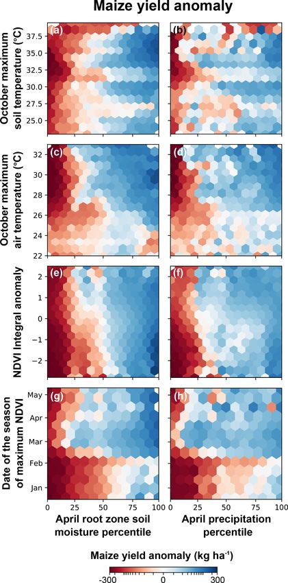
1830             N. Vergopolan et al.: Field-scale soil moisture for agricultural yield prediction and drought monitoring

  c. Height bands – defined by the height above nearest           2.3.1   Training data and feature engineering
     drainage and define the primary flow directions and sur-
     face temperature gradient.                                   To train the RF model, we used the Post-Harvest Surveys
                                                                  (PHSs) database of maize yields (in square kilometers). This
 d. HRUs – defined by multiple soil, vegetation, and land         database comprises household survey data of ∼ 13 000 farm-
    cover characteristics, and it represents the smallest mod-    ers’ self-reported harvested maize (in kilograms or total bags
    eling units.                                                  of the crop) and respective cultivated area (in hectares). The
                                                                  data were collected at the end of each harvesting season by
   With this hierarchical setup, HydroBlocks handles
                                                                  Zambia’s Central Statistical Office (a division of the Min-
mass/energy exchanges within a modeling unit (at a cer-
                                                                  istry of Agriculture and Livestock) from 1991 to 2005, in
tain scale) separately from the exchanges between units at
                                                                  2007 and 2008, and from 2011 to 2014. Due to privacy and
that scale. This enables full and realistic horizontal coupling
                                                                  data uncertainties, the observations were only available ag-
while ensuring computational efficiency.
                                                                  gregated to the district level (∼ 10 000 km2 ). In this work,
   We deployed the HydroBlocks to simulate root zone soil
                                                                  to match the period of availability for remotely sensed pre-
moisture and soil temperature from surface to 1.5 m depth
                                                                  dictors, we used the PHS data from 2000–2018. This re-
at 3 h 30 m resolution between 1981–2018. As data inputs,
                                                                  sulted in a total of 527 observations from 70 districts and
we used hourly 9 km meteorological inputs from ERA5-
                                                                  8 years. To train and evaluate the model, we used a year-
Land (Muñoz-Sabater et al., 2021) (rainfall, 2 m air tem-
                                                                  based cross-validation approach. This approach relies on se-
perature, longwave radiation, shortwave radiation, wind, sur-
                                                                  lecting a given year to evaluate the model and train it on all
face pressure, and specific humidity derived from dew point).
                                                                  the other years. This is performed for each of the 8 years
ERA5-Land is a state-of-the-art global reanalysis product
                                                                  independently, with the average statistics representing the
that was chosen because of its high spatial resolution and
                                                                  overall cross-validation performance. To train the model, we
overall good performance in representing rainfall and soil
                                                                  used a range of static and dynamic variables with time, as
moisture dynamics (Beck et al., 2021). To parameterize the
                                                                  described in Table 1.
HydroBlocks, we also used 30 m topography (Shuttle Radar
                                                                     From these static and dynamic predictors, we identified
Topography Mission – SRTM; Farr et al., 2007), 20 m land
                                                                  103 initial predictors. Of the many challenges of working
cover type (European Space Agency Climate Change Initia-
                                                                  with multisource and multiscale data sets, one is the spatial
tive – ESA-CCI), and 250 m soil properties (SoilGrids; Hengl
                                                                  scale mismatch of input data (20 m to 9 km resolution). To
et al., 2017) to derive the soil hydraulic parameters via pedo-
                                                                  reconcile these different scales and calculate a district-level
transfer functions. Although not calibrated, previous valida-
                                                                  value for each predictor, we masked out the non-cropland
tion work compared HydroBlocks soil moisture simulations
                                                                  pixels and calculated its area-weighted average based on the
with in situ observations over similar climates, and results
                                                                  cropland location/area in each district. Despite the large dis-
showed that the model represents the spatial and temporal
                                                                  trict areas, the use of these area-weighted averages at only
variability of in situ soil moisture measurement as field scale
                                                                  the agricultural areas helped to remove the influence from
and regional scale, with comparable performance to satellite
                                                                  the surrounding non-cropland areas (i.e., grasslands, water
estimates (Vergopolan et al., 2020; Cai et al., 2017), provid-
                                                                  bodies, and urban areas), while accounting for the spatial
ing reasonable confidence in the variability of the yield esti-
                                                                  variability of each predictor in the district. Lastly, each pre-
mates derived in this study.
                                                                  dictor was normalized based on the maximum and minimum
2.3    Modeling maize yields at district scale and                values. We used NDVI retrievals from Moderate Resolution
       mapping yields at field scale                              Imaging Spectroradiometer (MODIS) instead of Landsat be-
                                                                  cause of the lower cloud coverage and a shorter revisit time.
To model and predict maize yield dynamics at the field scale,     In Zambia, cloud coverage between December to February
we trained a random forest model on district-level, survey-       was, on average, 50 % for Landsat and 30 % for MODIS.
based maize yield data, high-resolution HydroBlocks simu-
lations, remotely sensed vegetation index, meteorological re-     2.3.2   Random forest regressor for yield modeling
analysis data, and other static information on the landscape.
Section 2.3.1 presents the data sets and predictor descrip-       Machine learning models have been widely applied for crop
tions. Section 2.3.2 presents the RF model setup and eval-        yield prediction (Chlingaryan et al., 2018). Random forest
uation. Section 2.3.3 presents the recursive feature elimina-     regressors are used with geospatial hydroclimate and satel-
tion approach applied to select and rank predictors. Lastly,      lite data to predict maize yields at fine scales (Aghighi
Sect. 2.3.4 presents how the RF model was deployed to pre-        et al., 2018; Khanal et al., 2018; Jeong et al., 2016; Fol-
dict annual maize yields in Zambia at the field level and the     berth et al., 2019). Advantages of RF regression models are
analysis performed to assess the yield’s spatial variability.     their high predictive accuracy, even when trained on small,
                                                                  nonlinear, and collinear data sets, their robustness to out-
                                                                  liers, and their ability to avoid overfitting (Breiman, 2001;

Hydrol. Earth Syst. Sci., 25, 1827–1847, 2021                                      https://doi.org/10.5194/hess-25-1827-2021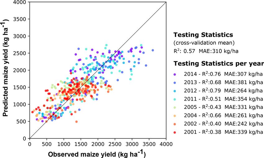
N. Vergopolan et al.: Field-scale soil moisture for agricultural yield prediction and drought monitoring                                  1831

Table 1. List of the data sets and the predictors derived to train the random forest model.

     Data set               References                      Predictors description                                               Type
     Land cover             20 m; ESA-CCI (2016)            The land cover classification was used to identify cropland areas    Static
                                                            (assuming that all croplands produce maize) and the percentage
                                                            coverage of non-agricultural cover types in 250 m pixels.
     Topography             30 m; SRTM (Farr et al.,        From elevation, we derived slope, aspect, topographic index,         Static
                            2007)                           and the height above the nearest drainage.
     Soil properties        250 m; SoilGrids (Hengl         Clay, sand, silt, and organic matter content, and the following      Static
                            et al., 2017)                   variables were derived using pedotransfer functions (Saxton and
                                                            Rawls, 2006): soil saturation, field capacity, wilting point, soil
                                                            water storage, and hydraulic conductivity calculated using pe-
                                                            dotransfer functions.
     Climatology:           1 km; WorldClim2 (Fick          Climatology of air temperature and precipitation during the          Static
     – Precipitation        and Hijmans, 2017)              growing season.
     – Air temperature
     Socioeconomic:         1 km; 2010 GDP (Bank,           GDP and population density as proxies for access to finance,         Static
     – GDP                  2012) and 2010 population       technology, and infrastructure.
     – Population           (CIESIN, 2017)
     Vegetation index:      250 m; MODIS MOD13Q1            Maximum growing season NDVI, date of maximum NDVI, and               Dynamic
     – NDVI                 (2000–2018)                     seasonal NDVI integrals calculated by using a smoothing func-
                                                            tion to fill the missing NDVI values and to remove outliers fol-
                                                            lowed by a Savitzky–Golay (SG) filter (Chen et al., 2004).
     Meteorological:        9 km monthly; ERA5-Land         Growing season and the monthly average together with mini-           Dynamic
     – Precipitation        (Muñoz-Sabater et al.,          mum and maximum estimates of air temperature and precipita-
     – Air temperature      2021)                           tion.
     Hydrological:          30 m     monthly;      Hy-      Seasonal and monthly average together with minimum and               Dynamic
     – Soil moisture        droBlocks (this study)          maximum root zone soil moisture, relative root zone soil mois-
     – Soil temperature                                     ture, and soil temperature from the HydroBlocks LSM.

Archer and Kimes, 2008; Wylie et al., 2019). Dealing with                 (i) identify and rank the most important predictors of maize
data collinearity is particularly important for yield predic-             yields and (ii) to determine which of the predictors could be
tion because often the meteorologically, hydrologically, and              removed. Removing non-predictive variables is particularly
vegetation-based predictors are interconnected (Archer and                helpful as it can improve model accuracy, and it mitigates the
Kimes, 2008; Wylie et al., 2019).                                         model’s tendency to overfit, while the smaller data volume
   To identify the optimal RF architecture, we performed a                reduces the computational cost.
grid search on the possible combinations of relevant hyper-                  The RFE is an iterative process. At each iteration, the
parameters, namely number of trees, maximum depth of the                  model is trained, the importance of each predictor calculated
trees, the minimum number of samples required to split an                 and ranked, and the least important predictor is removed
internal node, the minimum number of samples required to                  (Gregorutti et al., 2016). This process continues until a con-
be at a leaf node, and the number of bootstraps of predictors.            vergence criterion is met. In our implementation, as an eval-
The best hyper-parameter combination was selected based on                uation metric, we used the average maize yield R 2 of year-
the average mean square error (MSE) of a threefold cross-                 based cross-validation. The importance of each predictor was
validation on the training sample. We further evaluate the                calculated based on the difference between the R 2 of the
model’s overall performance by calculating the mean abso-                 model with the predictor and of the model without the predic-
lute error (MAE) and the coefficient of determination (R 2 )              tor. This iterative process of retraining and assessing the rel-
performance using a year-based cross-validation approach.                 ative importance of each predictor ensures that the least im-
                                                                          portant predictor is consistently removed and that discarded
2.3.3   Predictor importance and selection                                variables either do not contribute to or degrade model per-
                                                                          formance. Variable removal ceased once this R 2 difference
Using the district-level PHS yield data and the RF model, we              fell below 0.001 (see Table S1 in the Supplement for a full
performed a recursive feature elimination (RFE) analysis to

https://doi.org/10.5194/hess-25-1827-2021                                                Hydrol. Earth Syst. Sci., 25, 1827–1847, 2021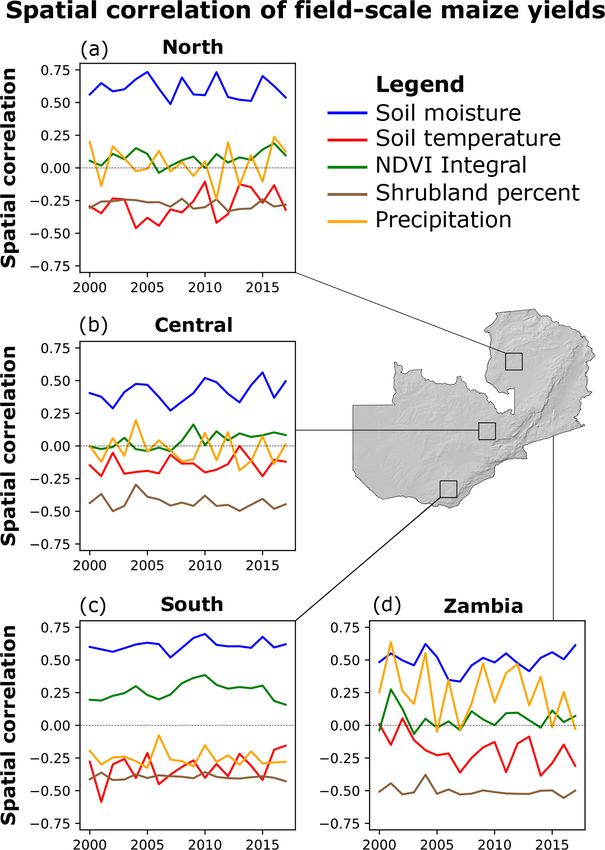
1832              N. Vergopolan et al.: Field-scale soil moisture for agricultural yield prediction and drought monitoring

description of the RFE process). The RFE process applied to          Spatial variability of field-scale maize yields and main
the 103 predictors (Sect. 2.3.1) resulted in the retention of 27     predictors
important predictors.
    In addition to variable selection, we performed a sensi-         The spatial patterns and spatial variability in maize yields
tivity analysis to quantify the relative value of hydrology-         can be driven by hydroclimatic conditions, soil properties, to-
based predictors (soil moisture and soil temperature) and            pography, and also farmer management (such planting date,
meteorology-based predictors (precipitation and air temper-          seed choice, use of fertilizers, irrigation, etc.). Consequently,
ature) in predicting district-level maize yields. For this ex-       droughts can impact the landscape differently. To quantify
periment, we trained the RF model, applied RFE, and iden-            the strength of each predictor in driving the spatial variabil-
tified the most important predictors of three different predic-      ity in maize yields at the local scale, we calculated the spa-
tor sets, as shown in Table 2. For each case, we quantified          tial Pearson correlation between the field-scale yields and the
the final R 2 year-based cross-validation performance and the        most important predictors. The time series of spatial correla-
delta R 2 importance of each predictor. We then compared             tion was calculated for each year over the entire country and
the change in performance with and without meteorology-              for three smaller domains (of 50 km by 50 km) in the north,
and hydrology-based predictors with respect to the bench-            central, and south of the country.
mark. We also compared the relative importance of different
predictors in each of the cases.                                     2.4   Characterizing the relationship between field-scale
                                                                           yields and drought indicators
2.3.4   Predicting maize yield at the field scale
                                                                     The predictor importance analysis (Sect. 2.3.3) identified the
Previous work showed that RF models are able to success-             most influential variables impacting maize yields at the dis-
fully model fine-scale crop yields from coarse-scale, phys-          trict scale. To gain further insight into the potential effec-
ically based crop models estimates, assuming that the fine-          tiveness of these variables as drought impact indicators, we
scale predictors are representative of the fine-scale yield vari-    compared how they varied with the spatially co-located de-
ability (Folberth et al., 2019). Similarly, we deployed the          trended maize yields, hereafter called anomalies. This allows
trained RF model to predict maize yields at 250 m resolution,        us to characterize the relationship between these indicators
considering that predictors and model parameters that repre-         (e.g., dry and hot) versus local losses or gains in maize yields.
sent the yield spatiotemporal dynamics at the district scale            The drought indicator variables, shown in Table 3, were
can represent yield dynamics at the field scale.                     identified based on the three most important predictors (result
   To this end, we first identified all 250 m grid cells that have   from Sect. 3.2) and three (respective) commonly used indica-
at least 50 % cropland coverage according to our fractional          tors. Temperatures and date of NDVI peak were used in their
land cover map derived from the ESA-CCI data (Table 1;               original units. For NDVI integrals, for each grid, we used the
Fig. S1), which resulted in ∼ 1 M grid cells. Since maize is         temporal anomaly relative to the 2000–2018 mean. For soil
Zambia’s dominant crop (Ng’ombe, 2017), and it accounts              moisture and precipitation, drought indices were constructed
for 60 % of the planted area, we assume that all the identi-         from monthly values and converted to the empirical per-
fied cropland areas are maize fields. Similar to the predictor       centile. The empirical percentile was calculated for each time
set, we used the location/area of the cropland fields to cal-        step and grid cell and based on the monthly historical records
culate the area-weighted average of each predictor. We used          (1981–2018) for that location/month (Sheffield, 2004). By
our best RF model to predict the annual maize yield at each          using percentiles, rather than absolute values, drought events
250 m grid cell over Zambia between 2000 to 2018.                    can be compared in space and time despite their local char-
   To characterize the spatiotemporal distribution of field-         acteristics.
scale maize yields estimates derived from the RF model, we              By comparing how each drought indicator varied with
generated maps of mean annual yields and their temporal co-          the yield anomalies, this approach allowed us to character-
efficient of variation. We also calculated maps of maize yield       ize the relationship between these indicators versus local
trends between 2000–2018 to identify the locations where             losses (or gains) in maize yields. We delineated potential
increases in yields were larger. As an example, to quantify          drought thresholds for soil moisture and precipitation per-
the spatial distribution of losses in yield due to drought, we       centiles and quantified the mean expected yield losses asso-
calculated the relative change in yields for the 2015–2016 El        ciated with each threshold. Second, we compared how each
Niño season and compared it to FAO survey estimates (Al-             of the drought indicators co-varied with each other and with
fani et al., 2019). Despite the sampling difference between          maize yield anomalies. This allowed us to quantify what the
the surveyed and predicted field-scale yields, we evaluate           expected yield losses (or gains) are under dry and hot versus
the estimated field-scale yields by comparing the field-scale        wet and hot conditions and to identify in which conditions
yields aggregated to the district level with district-level PHS      yield losses are driven by water deficits and/or temperature
survey yield data. We computed the temporal R 2 and MAE              stress.
and the mean spatial Pearson correlation.

Hydrol. Earth Syst. Sci., 25, 1827–1847, 2021                                         https://doi.org/10.5194/hess-25-1827-2021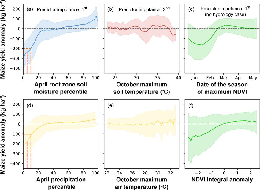
N. Vergopolan et al.: Field-scale soil moisture for agricultural yield prediction and drought monitoring 1833
Table 2. Predictor sets applied to the maize yield modeling sensitivity experiments.
Case Name Description Total predictors
1 All predictors All the predictors as a benchmark 103
2 No meteorology All the predictors, except the precipita- 70
tion and air temperature predictors
3 No hydrology All the predictors, except the soil mois- 61
ture and soil temperature predictors
Table 3. List of the six drought impact indicators used in the crop losses analysis, where three are the most predictive variables (identified
by the predictor importance analysis) and three are, respectively, commonly used indicators.
Indicator Variables
conditions Most predictive Commonly used
Dry/wet Root zone soil moisture (April) Precipitation (April)
Cool/hot Max soil temperature (October) Max air temperature (October)
Plant health Date of NDVI peak (season) NDVI Integral (season)
3 Results predictors of yield (Fig. 3). In the first two sensitivity tests,
in which Hydroblocks variables were included, soil mois-
3.1 Hydrological simulations at field scale ture and temperature variables provided five or six of the top
seven predictors, while removing soil moisture and temper-
HydroBlocks-simulated root zone soil moisture and soil tem- ature variables as predictors (case 3) resulted in the largest
perature at 30 m resolution reveal substantial spatial variabil- drop in overall model R 2 (0.06 and 0.08). On the other hand,
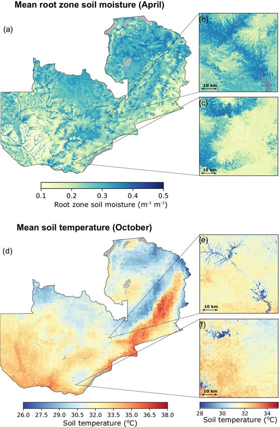
ity at both the national and local scales. Figure 1 shows the removing meteorological variables resulted in relatively lit-
mean April root zone soil moisture and October soil temper- tle loss of model explanatory power, with an R 2 drop of only
ature, since these variables are the most important predictors 0.02 between cases 1 and 2.
of yield (Sect. 3.2). At the national scale, wet and cooler con- In terms of specific variables, cases 1 and 2 both showed
ditions are observed in the northern parts of the country and that the mean relative soil moisture in April was the strongest
near river valleys, while the south and southeast show dis- predictor of yield, followed by precipitation climatology, Oc-
tinctly dry and hot conditions. National- and local-scale vari- tober and February soil temperatures, and then March soil
ations (Fig. 1 inset) reflect the interactions of meteorological moisture (Fig. 3). There are two static variables that appear
conditions with the landscape, highlighting the influence of to have some strong influence as well, namely shrubland
topography, soil properties, and vegetation cover on the spa- percentage, which is ranked third in case 2, and precipita-
tial variability of hydrological processes. tion climatology, which represents the spatial distribution of
rainfall, appearing second in case 1 and accounts for an R 2
3.2 District-level maize yield modeling and importance drop of 0.02 if removed from the model. Besides this vari-
of predictors able, no other meteorologically derived variable, including
all the dynamic measures, ranks highly in the presence of Hy-
The best-performing RF model was able to predict the val- droBlocks variables. The highest of these is December mean
ues of the district-level yield data, with an average mean ab- air temperature, which ranks 10th in case 1. Removing Hy-
solute error of 310 kg ha−1 and an R 2 of 0.57 (year-based droBlocks variables (case 3) increases the influence of these
cross-validation). Figure 2 shows the comparison between variables, but they still remain less predictive than the static
observed and predicted yields for each year (with the model precipitation climatology, while the dynamic vegetation mea-
trained on data of all the other years). The model captures sures, date of maximum NDVI, and the corresponding value
the overall patterns of district-level maize yields but with a are, respectively, the first and sixth most influential. NDVI-
tendency to underestimate maize yields above 2500 kg ha−1 derived variables otherwise rank 12th in case 1 and were not
in the recent years (e.g. 2011–2014) and overestimate low retained in case 2.
yields in the earlier years (e.g. 2001–2004).
The recursive feature elimination process, combined with
the sensitivity analysis (Table 2), revealed that soil moisture
and soil temperature variables were consistently the strongest
https://doi.org/10.5194/hess-25-1827-2021 Hydrol. Earth Syst. Sci., 25, 1827–1847, 2021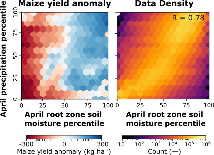
1834              N. Vergopolan et al.: Field-scale soil moisture for agricultural yield prediction and drought monitoring

Figure 1. April root zone soil moisture and October soil temperature were the most predictive variables in the RF model. Panels (a) and (b)
show respective mean values (2000–2018), at the 30 m spatial resolution, as simulated by the HydroBlocks land surface model. Large lakes
are excluded from the simulations (gray areas).

3.3    Field-scale maize yields for Zambia                              southern regions (Fig. 4a), which reflects the spatial distribu-
                                                                        tion of mean rainfall. Figure S6 in the Supplement shows
At the field scale, RF-predicted maize yields averaged                  time series of the predicted yields for different locations
1557 kg ha−1 (±219 kg ha−1 ) for the 2000–2018 period. As               across the country. In terms of the temporal coefficient of
expected, we observe higher average maize yields in the                 variation (Fig. 4d), yield variability is highest in the central,
northern parts of the country and lower average yields in the

Hydrol. Earth Syst. Sci., 25, 1827–1847, 2021                                             https://doi.org/10.5194/hess-25-1827-2021
N. Vergopolan et al.: Field-scale soil moisture for agricultural yield prediction and drought monitoring 1835 Figure 2. Comparison between observed and predicted maize yields at the district scale. The predictions were obtained by training a ran- dom forest model with survey-based maize yield data and fine-scale geospatial environmental data sets. Each color shows the maize yield evaluation for a given year (trained on data of the other years). Figure 3. The most important predictors for maize yield at the district scale. The predictors were selected and ranked via recursive feature elimination, with the importance rank shown in terms of delta R 2 . Results are shown for case 1 (considering all the variables), case 2 (without precipitation and air temperature predictors), and case 3 (without soil moisture and soil temperature predictors). Each color represents different categories of predictors data. https://doi.org/10.5194/hess-25-1827-2021 Hydrol. Earth Syst. Sci., 25, 1827–1847, 2021
1836 N. Vergopolan et al.: Field-scale soil moisture for agricultural yield prediction and drought monitoring
southern, and eastern parts of the country and lowest in north- Field-scale spatial variability of yields and dominant
ern and northwestern Zambia. In general, there is an inverse predictors
relationship between mean annual yields and their coefficient
of variation (Fig. S2 in the Supplement); however, there are As observed in Fig. 5b, droughts impact yields differently
several notable departures. For example, a landscape-level across the landscape. To quantify to what extent the spa-
view in central Zambia reveals areas of moderate to high tial variability in the hydroclimate and landscape conditions
yields (Fig. 4b) with corresponding moderate to high lev- are driving the spatial variability in the yields, we calcu-
els of variability (Fig. 4f), due to proximity to rivers and lated the spatial correlation between the field-scale yields and
extensive floodplains, where inundation is frequent. The op- the dominant predictors (Fig. 6). The spatial correlation was
posite pattern is seen in southern Zambia, where portions of calculated each year, to assess whether these associations
the landscape show low yields and relatively low variability changed inter-annually, and over different locations (the en-
(Fig. 4c and e) due to more consistently dry conditions. tire country and for 50 km×50 km boxes in southern, central,
Analyzing the change in maize yields trends for the pe- and northern Zambia) to assess how the relationships change
riod 2000–2018 (Fig. 4g, h, and i), we found that, on regionally.
the whole, maize productivity increased by 3.5 kg ha−1 yr−1 Soil moisture exhibited the largest impact on the spa-
(±4.6 kg ha−1 yr−1 ). The gain was more prominent in the tial variability in yields, with the highest spatial correlation
northern and central parts of the country, particularly in the across all three subregions and the entire country (Fig. 6a–d).
floodplains (Fig. 4i), rising to 15 kg ha−1 yr−1 , while there Soil temperature and shrubland percent are negatively corre-
was little change in southern Zambia. The productivity also lated with yield. The relative ranking and temporal dynam-
tends to be higher at the locations near floodplains (Fig. 4i). ics of the spatial correlations are generally consistent across
Nonetheless, the overall yield gains rates observed were far regions, although the strength of correlation varies between
behind than the rates required to match the 12 000 kg ha−1 regions, with close to zero correlation for most predictors
Zambia yield potential (Mueller et al., 2012). in the central and northern regions. Given its coarser spatial
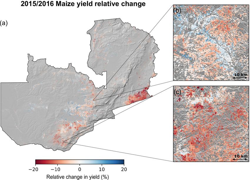
During the 2015–2016 El Niño drought, Zambian agri- scale and smoother spatial variability, precipitation climatol-
cultural production was severely impacted with overall ogy showed no spatial correlation with the field-scale yield
losses across the country. Our field-scale RF-predicted for each region, but strong correlations at the national scale
yields were able to capture these losses (Fig. 5). The due to the substantial spatial gradient. However, the high in-
countrywide predicted mean yield for 2015–2016 was terannual variability indicates the influence of other factors.
1514 kg ha−1 (±233 kg ha−1 ), which represents an over- With the exception of southern Zambia, NDVI showed a low
all loss of 84 kg ha−1 (±60 kg ha−1 ), or 5.3 %, relative to spatial correlation with yield over time.
2010–2014 mean. Predicted yield reductions were more
severe in southern and southeastern Zambia, with losses 3.4 The impact of drought on field-scale maize yields
of 200 kg ha−1 (15 %) across much of this area, reaching as
high as 522 kg ha−1 (28 %) (Fig. 5). These estimates align To examine the effectiveness of the six potential drought
with those of the 20 % losses estimated by the Food and indicators (Table 3), we evaluated the degree of influence
Agriculture Organization (FAO) for this same area during the that each indicator had on the anomalies of the predicted
2015–2016 El Niño drought (Alfani et al., 2019). However, field-scale yields (Fig. 7). Overall, the relationship between
when evaluating drought impact at the local scales (Fig. 5b these indicators and yield anomalies was highly nonlinear.
and c), we observe that drought impacts yield differently Soil moisture and precipitation percentiles capture the largest
across the landscape. Areas nearby to rivers and floodplains yield losses of all six indicators (Fig. 7a and d), with both
were less prone to crop losses (Fig. 5b), given the wetter and showing substantial negative anomalies below their 25th per-
cooler soil moisture conditions. centile values. Yield losses associated with low soil moisture
We compared the field-scale yield data aggregated to the conditions are larger and more certain than those related to
district level with the PHS survey district-level yield data. low precipitation. For instance, yield losses associated with
We obtained a Pearson correlation of 0.67 (R 2 = 0.46) and the 10th soil moisture percentile (202 ± 134 kg ha−1 ) were
an MAE of 450 kg ha−1 . In terms of spatial patterns, aggre- 89 % greater than those related to the 10th precipitation per-
gated field-scale yield and PHS have a spatial correlation of centile (107±135 kg ha−1 ; orange dashed lines in Fig. 7a and
0.84. This strong spatial relationship is also evident in the d). At the fifth percentile (red dashed line in Fig. 7a and d),
PHS and estimated z scores shown in Fig. S3 in the Supple- average soil-moisture-related yield loss (235 ± 128 kg ha−1 )
ment. The weak strength and limitations of this aggregated was 26 % greater than the yield loss associated with the pre-
data comparison are discussed in Sect. 4.4. cipitation (187 ± 161 kg ha−1 ) and, furthermore, had a 20 %
narrower confidence interval.
Negative NDVI integral anomaly and early NDVI peak
date were also associated with yield reductions (Fig. 7c and
f). The strongest and most certain of these was the date of
Hydrol. Earth Syst. Sci., 25, 1827–1847, 2021 https://doi.org/10.5194/hess-25-1827-2021N. Vergopolan et al.: Field-scale soil moisture for agricultural yield prediction and drought monitoring 1837 Figure 4. Annual maize yields (a), coefficient of variation (d), and maize yield trends (g) for the period between 2000–2018 estimated using a random forest model. Each magnified panel (b, c, e, f, h, i) shows the respective estimates at a 250 m resolution for a 50 km × 50 km area. peak NDVI, which resulted in yield anomalies when maxi- In contrast to the previous two indicators, there was lit- mum NDVI occurred before March, with the largest reduc- tle variation in yield anomalies associated with soil and air tions (164 ± 146 kg ha−1 ) occurring for peak dates between temperature, although the uncertainty in anomalies increased January and February. Negative NDVI integral anomalies with both measures. However, we observe nearly consistent also showed substantial but more uncertain yield losses. For yield losses with October maximum soil temperatures above example, an NDVI integral anomaly of −2 identified a yield 37.5 ◦ C, which is near known critical temperature thresholds loss of 140 ± 210 kg ha−1 . for maize (Luo, 2011; Schauberger et al., 2017). https://doi.org/10.5194/hess-25-1827-2021 Hydrol. Earth Syst. Sci., 25, 1827–1847, 2021
1838              N. Vergopolan et al.: Field-scale soil moisture for agricultural yield prediction and drought monitoring

Figure 5. (a) Relative change in maize yields (in percent) for the 2015–2016 season with respect to 2010–2014 mean. Each magnified panel
(b, c) shows the respective data at a 250 m resolution for a 50 km by 50 km area.

   To gain further insight into the conditions (e.g., hot and         4     Discussion
dry vs. hot and wet) associated with yield losses, in Fig. 8
we compared how the yield anomalies co-varied with pair-              4.1    Key findings
wise drought indicators. For example, Fig. 8a shows what
the mean yield anomaly associated with its respective Octo-           We presented a modeling framework that combines physi-
ber maximum temperature and April root zone soil moisture             cally based, hyper-resolution land surface modeling and ma-
is. As expected from previous findings (Fig. 7), soil mois-           chine learning for maize yield prediction at the field scale.
ture (Fig. 8a, c, and e) and precipitation (Fig. 8b, d, and f)        Our work advances on previous approaches by integrating
percentiles are the dominant influences on maize yield re-            field-scale hydrological variables into yield prediction and
sponses. Both indicators show similar patterns, but the yield         by more effectively quantifying yield sensitivity to drought.
responses associated with precipitation are noisier. Extreme          Our key findings are as follows:
soil temperature (Fig. 8a and b) and air temperature (Fig. 8c
                                                                          – Model skill. The modeling approach that we devel-
and d) only lead to yield losses (red) when the soil moisture
                                                                            oped was able to estimate maize yields at district scale
and precipitation percentiles are low (< 25th). High temper-
                                                                            with comparable skill (R 2 = 0.57; MAE = 310 kg ha−1 )
atures under wet conditions (top right corners in Fig. 8a–d)
                                                                            compared to state-of-the-art approaches based on mech-
show increased productivity (blue). Yield losses occur for the
                                                                            anistic yield models (e.g., Jin et al., 2017; Azzari et al.,
full range of NDVI peak dates when soil moisture and precip-
                                                                            2017) and with higher skill than standard empirical ap-
itation percentiles are below 10–15th, but when the peak date
                                                                            proaches based on weather variables or vegetation in-
is earlier than March, yield losses occur when soil moisture
                                                                            dices (Estes et al., 2013; Zhao et al., 2018).
and precipitation fall below their median values (Fig. 8g and
h). NDVI integral anomalies below zero and below median                   – Yield estimates. The field-scale results showed a mean
soil moisture values show a similar relationship with yield                 maize yield of 1557 kg ha−1 (±219 kg ha−1 ) across
(Fig. 8e), but this tendency was much weaker when assessed                  Zambia, with an overall increasing production trend of
with precipitation (Fig. 8f).                                               3.5 kg ha−1 yr−1 (±4.6 kg ha−1 yr−1 ) between 2000 and
                                                                            2018. The field-scale yields captured maize losses dur-
                                                                            ing the 2015–2016 El Niño drought at similar levels to
                                                                            losses reported by the FAO based on actual yield data
                                                                            (Alfani et al., 2019).

Hydrol. Earth Syst. Sci., 25, 1827–1847, 2021                                            https://doi.org/10.5194/hess-25-1827-2021
N. Vergopolan et al.: Field-scale soil moisture for agricultural yield prediction and drought monitoring 1839
ently across the landscape (Fig. 5), with most of the spa-
tial variability coming from soil moisture (Fig. 6).
4.2 Drivers of maize yields predictability
Soil moisture and precipitation
Soil moisture and soil temperature showed a strong contri-
bution to yield prediction because they represent the water
and temperature balances at the root zone, accounting for the
soil–water–plant interactions via infiltration, surface and sub-
surface flow, vertical drainage, water uptake by plants, and
evaporation. Consequently, in our sensitivity experiments,
in case 1 and case 2, the meteorological predictors added
only minor improvements to yield prediction beyond the con-
tribution of root zone predictors, mainly because precipita-
tion does not necessarily translate into water availability for
plants. For example, rainfall from intense storms may con-
tribute mostly to runoff rather than infiltration, leading to a
spatial mismatch between where the water is supplied (pre-
cipitation) and where water is finally available to plants (soil
moisture). Furthermore, whilst temperature drives the atmo-
spheric demand for evapotranspiration, it does not reflect the
complexity of controls on transpiration, which are more wa-
ter limited (rather than energy limited) in drier regions such
as much of Zambia (Berg et al., 2016; Williams et al., 2012;
McNaughton and Jarvis, 1991).
Distinctions between atmospheric and root zone processes
are particularly important at the field scale, due to different
Figure 6. Time series of Pearson spatial correlation of maize yields natural scales of variability that influence crops in differ-
and the most important predictors. Panels show the spatial corre-
ent ways. Precipitation and air temperature operate mostly
lation within 50 km by 50 km boxes in (a) south, (b) central, and
(c) north of Zambia. Panel (d) shows the spatial correlation for the
at larger scales, with most of the spatiotemporal variability
entire country. coming from large-scale atmospheric circulation and large-
scale topographic features (Grayson and Blöschl, 2001). Soil
moisture, on the other hand, operates at multiple scales, in-
– Drivers of yield. We identified soil moisture as the main fluenced by the meteorological conditions, but with most of
driver of maize yield variability at both the district scale the spatial variability coming from the heterogeneity of the
and field scale. At the district scale, soil moisture was landscape (topography, soil properties, and land cover; Crow
followed in importance by soil temperature, shrubland et al., 2012; Famiglietti et al., 2008; Grayson and Blöschl,
percent coverage, and precipitation climatology. Time- 2001). By providing soil moisture and soil temperature esti-
varying meteorological predictors (precipitation and air mates at a spatial scale closer to its natural scale of variabil-
temperature) played a minor role. NDVI-based predic- ity, HydroBlocks allows for improved yield predictions. This
tors only showed meaningful contribution when soil is indicated by comparison of the joint distribution of soil
moisture and soil temperature predictors were absent. moisture and precipitation percentiles (Fig. 9), which shows
that most of the time their condition will be similar (0.78
– Drought impacts. There is a highly nonlinear behav- correlation), yet when they are different (due to the above
ior between drought indices and yield losses. However, reasons), soil moisture better captures losses in yield.
consistent maize losses are observed when soil mois- April soil moisture ranked as the strongest predictor of
ture or precipitation drop below the 25th percentile. At yield. April covers the grain-filling stage of the maize calen-
extreme dry conditions (fifth percentile), soil moisture dar in Zambia (∼ 35 d prior to maturity; Yonts et al., 2008),
identifies 26 % more losses with 21 % less uncertainty when soil moisture is critical for plants because of the large
than precipitation, providing an effective measure of water uptake demands (Yonts et al., 2008; Borras et al.,
drought impact. Significant yield losses are also pre- 2003). Despite the high greenness of the season (measured by
dicted when soil temperature exceeded 37.5 ◦ C in the vegetation indices such as NDVI, for example), if plants do
early growing season. Drought impacted yields differ- receive enough water in the reproductive period, then the cob
https://doi.org/10.5194/hess-25-1827-2021 Hydrol. Earth Syst. Sci., 25, 1827–1847, 20211840 N. Vergopolan et al.: Field-scale soil moisture for agricultural yield prediction and drought monitoring
Figure 7. The relationship between the field-scale maize yield anomalies with respect to the six drought indicators identified in Table 3.
Panels (a–c) show the most predictive variables, and panels (d–f) show the (respective) commonly used variables. Dark lines show the mean
values, and shades show the standard deviation. Red and orange dashed lines illustrate potential drought thresholds.
will not develop well, compromising productivity. Although son was low; otherwise, an overall yield gain is observed
several studies identified NDVI as the strongest predictors for (Fig. 8a). Thus, wet soil moisture conditions (e.g., irrigation)
maize (Table 1 in Funk and Budde, 2009; Johnson, 2016; Pe- could play an important role in mitigating extreme heat ef-
tersen, 2018; Karthikeyan et al., 2020), our sensitivity analy- fects (Troy et al., 2015; Thomas et al., 2020) and potentially
sis results (Fig. 3; case 3) showed that only in the absence of even increase productivity (Steward et al., 2018), such as ob-
soil moisture and soil temperature variables do NDVI-based served in Fig. 5b. Nonetheless, because of maize’s overall
variables emerge as strong predictors of yield. This is evi- sensitivity to elevated temperatures (Lobell and Field, 2007;
dent in Fig. 8e and g, which show that NDVI-based anoma- Lobell et al., 2013), soil temperature above 37.5 ◦ C would
lies have little sensitivity to change in yields when compared lead to yield losses despite the wet conditions in the late sea-
to soil moisture. This could also be a limitation of visible son (Fig. 8a and b).
satellite sensors in capturing under canopy plant–soil–water
dynamics. A further discussion on NDVI limitations is pre- Static landscape predictors
sented in Sect. 4.4.
In terms of the static predictors, shrubland ranked third in
Soil temperature and extreme heat case 2 as it may represent the heterogeneity of agricultural
landscapes. While high cropland percent could be associ-
Soil temperatures in October (sowing period) are also criti- ated with more homogenous agricultural fields (often as-
cal for controlling yields. When the rainy season is delayed, sociated with commercial farming), high shrubland percent
extreme temperatures in the early stages can potentially dam- may indicate a higher presence of fragmented agricultural
age seeds prior to their germination (Mulenga et al., 2016) or areas, reflecting poorer agricultural landscapes (from a phys-
cause an earlier start to the maize reproductive period, in- ical and management perspective) and, consequently, lower
creasing the susceptibility to heat and water stress (Harri- yields (Maggio et al., 2018). Figure S5 in the Supplement il-
son et al., 2011; Hatfield and Prueger, 2015). However, el- lustrates this relationship. On the other hand, actual shrub-
evated temperatures in the early season only lead to yield land/cropland mosaics may be more likely to be misclas-
losses when the soil moisture content at the end of the sea- sified as a cropland pixel (commission error), which could
Hydrol. Earth Syst. Sci., 25, 1827–1847, 2021 https://doi.org/10.5194/hess-25-1827-2021You can also read