Assessment of a full-field initialized decadal climate prediction system with the CMIP6 version of EC-Earth
←
→
Page content transcription
If your browser does not render page correctly, please read the page content below
Earth Syst. Dynam., 12, 173–196, 2021
https://doi.org/10.5194/esd-12-173-2021
© Author(s) 2021. This work is distributed under
the Creative Commons Attribution 4.0 License.

           Assessment of a full-field initialized decadal climate
          prediction system with the CMIP6 version of EC-Earth
              Roberto Bilbao1 , Simon Wild1 , Pablo Ortega1 , Juan Acosta-Navarro1 , Thomas Arsouze1 ,
           Pierre-Antoine Bretonnière1 , Louis-Philippe Caron1 , Miguel Castrillo1 , Rubén Cruz-García1 ,
               Ivana Cvijanovic1 , Francisco Javier Doblas-Reyes1,2 , Markus Donat1 , Emanuel Dutra3 ,
              Pablo Echevarría1 , An-Chi Ho1 , Saskia Loosveldt-Tomas1 , Eduardo Moreno-Chamarro1 ,
        Núria Pérez-Zanon1 , Arthur Ramos1 , Yohan Ruprich-Robert1 , Valentina Sicardi1 , Etienne Tourigny1 ,
                                              and Javier Vegas-Regidor1
                        1 BarcelonaSupercomputing Center, Jordi Girona 29, 08034 Barcelona, Spain
                 2 Institució
                            Catalana de Recerca i Estudis Avançats (ICREA), Passeig Lluis Companys 23,
                                                  08010 Barcelona, Spain
             3 Instituto Dom Luiz, Faculdade de Ciências, Universidade de Lisboa, 1749-016 Lisbon, Portugal

                                 Correspondence: Roberto Bilbao (roberto.bilbao@bsc.es)

                                Received: 28 August 2020 – Discussion started: 10 September 2020
                     Revised: 14 December 2020 – Accepted: 18 December 2020 – Published: 11 February 2021

      Abstract. In this paper, we present and evaluate the skill of an EC-Earth3.3 decadal prediction system contribut-
      ing to the Decadal Climate Prediction Project – Component A (DCPP-A). This prediction system is capable of
      skilfully simulating past global mean surface temperature variations at interannual and decadal forecast times
      as well as the local surface temperature in regions such as the tropical Atlantic, the Indian Ocean and most of
      the continental areas, although most of the skill comes from the representation of the external radiative forcings.
      A benefit of initialization in the predictive skill is evident in some areas of the tropical Pacific and North At-
      lantic oceans in the first forecast years, an added value that is mostly confined to the south-east tropical Pacific
      and the eastern subpolar North Atlantic at the longest forecast times (6–10 years). The central subpolar North
      Atlantic shows poor predictive skill and a detrimental effect of initialization that leads to a quick collapse in
      Labrador Sea convection, followed by a weakening of the Atlantic Meridional Overturning Circulation (AMOC)
      and excessive local sea ice growth. The shutdown in Labrador Sea convection responds to a gradual increase in
      the local density stratification in the first years of the forecast, ultimately related to the different paces at which
      surface and subsurface temperature and salinity drift towards their preferred mean state. This transition happens
      rapidly at the surface and more slowly in the subsurface, where, by the 10th forecast year, the model is still
      far from the typical mean states in the corresponding ensemble of historical simulations with EC-Earth3. Thus,
      our study highlights the Labrador Sea as a region that can be sensitive to full-field initialization and hamper the
      final prediction skill, a problem that can be alleviated by improving the regional model biases through model
      development and by identifying more optimal initialization strategies.

Published by Copernicus Publications on behalf of the European Geosciences Union.
174                                                                      R. Bilbao et al.: EC-Earth3 decadal prediction system

1   Introduction                                                     (SST) and upper-ocean heat content (OHC) (e.g. Pohlmann
                                                                     et al., 2009; Keenlyside et al., 2008; Robson et al., 2018;
Interest in seasonal to decadal climate predictions has              Yeager et al., 2018), although these same systems show a
grown in recent years due to their potential to provide rel-         limited capacity to predict the climate of the neighbouring
evant climate information for decision-making in differ-             continents, which might be related to an inaccurate represen-
ent socio-economic sectors (e.g. Suckling, 2018; Solaraju-           tation of key teleconnection mechanisms (e.g. Goddard et al.,
Murali et al., 2019; Merryfield et al., 2020). Scientifically,       2013; Doblas-Reyes et al., 2013). Encouragingly, a recent
climate predictions have provided novel ways of evaluating           study by Smith et al. (2020) has shown that decadal predic-
and comparing climate simulations with observations and              tions contributing to the Coupled Climate Model Intercom-
improve our understanding of the intrinsic predictability of         parison Project Phase 6 (CMIP6) can be skilful at predicting
the climate system, including the key mechanisms operating           the low-frequency variations of the North Atlantic Oscilla-
at interannual to decadal timescales.                                tion (NAO), the leading mode of the winter atmospheric cir-
   On these timescales a large part of the predictable sig-          culation in the Northern Hemisphere (Hurrell, 1996), when
nal of climate variations during the observational period is         considering a large multi-model ensemble. Similarly promis-
attributable to changes in external radiative forcings (i.e.         ing results for predicting the NAO at multi-annual timescales
changes in the climate system energy balance), which can             has also been shown for the Decadal Prediction Large En-
be of natural (e.g. solar irradiance and volcanic aerosols) or       semble from the National Center for Atmospheric Research
anthropogenic (e.g. greenhouse gas concentrations, land use          (NCAR) (Athanasiadis et al., 2020). Smith et al. (2020) also
changes and anthropogenic aerosols) origin. For example,             conclude that the NAO and the related climate signals over
at the global scale most of the surface temperature changes          Europe might be more predictable than models suggest and
can be explained by the warming trend caused by the in-              that large ensembles of predictions are necessary as current
creasing atmospheric greenhouse gas concentrations, which            forecast systems can strongly underestimate the predictable
are partly compensated for by a parallel increase in anthro-         signal (Scaife and Smith, 2018).
pogenic aerosols (e.g. Bindoff et al., 2013), and the spo-              To reinforce the inter-comparability of the results and al-
radic cooling episodes that followed the major volcanic erup-        low for the exploitation of large multi-model ensembles, the
tions of Mt. Agung (1963), El Chichón (1982) and Pinatubo            decadal climate prediction community has promoted the de-
(1991) (e.g. Ménégoz et al., 2018; Hermanson et al., 2020).          velopment of coordinated climate prediction exercises. The
Estimates of past changes in these radiative forcings are pre-       Decadal Climate Prediction Project (DCPP; Boer et al.,
scribed as boundary conditions to drive the so-called histor-        2016), as part of the Coupled Climate Model Intercompar-
ical climate simulations, which investigate the influence of         ison Project Phase 6 (CMIP6; Eyring et al., 2016), and build-
the forcings on the recent climate variations. These exper-          ing upon CMIP5 (Taylor et al., 2012) and the efforts of
iments are continued into the future as climate projections          previous projects (e.g. SPECS and ENSEMBLES), provides
with imposed anthropogenic radiative forcings that follow            such a framework for addressing different aspects and current
different theoretically derived socio-economic emission sce-         knowledge gaps in decadal climate prediction. DCPP-A is
narios (O’Neill et al., 2016).                                       the main component and consists of an ensemble of decadal
   The other main source of predictability originates from in-       hindcasts, initialized at yearly intervals from 1960 up to 2018
ternal variability, in particular in the slowly evolving com-        using prescribed CMIP6 external radiative forcings.
ponents of the climate system, i.e. the ocean (e.g. Meehl               A crucial step to maximize the skill of decadal predictions
et al., 2009). Besides being driven with external radiative          is the realistic initialization of the climate system. It is of ma-
forcings, climate predictions are also initialized from the ob-      jor importance to produce physically consistent initial condi-
served state to put the model in phase with observed internal        tions that reflect the observed state of climate as faithfully as
variability. Predictive skill of real-time forecast systems is as-   possible: in particular, the three-dimensional ocean tempera-
sessed by producing retrospective predictions (or hindcasts),        ture and salinity fields, which determine the basin-wide den-
which are then contrasted with observations. At seasonal to          sity gradients and through them the large-scale ocean circula-
annual timescales, hindcasts show high levels of predictive          tions and transports, which are essential for predictability on
skill for El Niño–Southern Oscillation (ENSO) (e.g. Barn-            decadal timescales (e.g. Meehl et al., 2014; Brune and Baehr,
ston et al., 2019). On decadal timescales, many climate mod-         2020). However, observational records are sparse in time and
els have also shown the capacity to skilfully predict the At-        space, especially in the deep ocean and before modern instru-
lantic multidecadal variability (AMV) (e.g. García-Serrano           ments (such as ARGO floats) were introduced, which poses
et al., 2015) and, to a lesser extent, the Interdecadal Pacific      a challenge with respect to accurately constraining the initial
Oscillation (IPO) (e.g. Mochizuki et al., 2009; Chikamoto            state from observations. For this reason, a typical approach
et al., 2015; Meehl et al., 2015, 2016). The North Atlantic          in climate prediction is to use initial conditions from ocean
Ocean, more precisely the Subpolar Gyre, has been identified         and atmosphere reanalysis. These are produced with data as-
as a region where different retrospective prediction systems         similation techniques that ensure a dynamically consistent
skilfully predict the evolution of sea surface temperatures

Earth Syst. Dynam., 12, 173–196, 2021                                                    https://doi.org/10.5194/esd-12-173-2021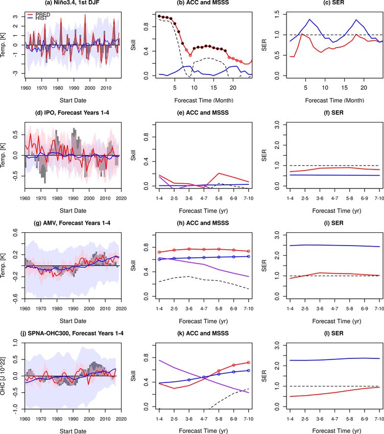
R. Bilbao et al.: EC-Earth3 decadal prediction system                                                                            175

estimation of the climate state that takes observational un-        range of different techniques have been used to produce the
certainties into account.                                           reconstructions, from classical nudging approaches based on
   Due to structural errors in climate models and biases in         Newtonian relaxation (e.g. Sanchez-Gomez et al., 2016; Ser-
their climatologies, when initialized from the observed state,      vonnat et al., 2015) to more complex and computationally
predictions suffer from initial shocks and drifts (e.g. Magnus-     expensive methods like the ensemble Kalman filter approach
son et al., 2012; Sanchez-Gomez et al., 2016; Kröger et al.,        (e.g. Counillon et al., 2014; Dai et al., 2020), which take as-
2018; Meehl et al., 2014). In this paper, initial shocks refer      pects of the observational uncertainty into account.
to abrupt changes that occur soon after initialization as a re-        The aim of this paper is to present and analyse a decadal
sult of the adjustment of the climate model to the initial state    prediction system within the EC-Earth3 model contributing
and/or to incompatibilities between the initial conditions of       to the CMIP6 DCPP-A. The paper is organized as follows:
the different components, whereas model drift refers to the         Sect. 2 provides a description of the EC-Earth3 forecast sys-
mean evolution of the forecasts towards an imperfect mean           tem, the initialization approach considered, the skill evalua-
model climate, which is tightly linked to how systematic            tion metrics and the observational datasets used. In Sect. 3,
model errors develop (Sanchez-Gomez et al., 2016). When             we characterize the predictive capacity for the surface tem-
their occurrence is consistent across start dates, initial shocks   peratures and investigate the importance of the initialization
(which are not present in all systems) are part of the drift        on surface temperatures, upper-ocean heat content and sev-
and can even condition its development. Two main initial-           eral interannual to decadal indices of climate variability, fol-
ization approaches are often used: “full-field initialization”,     lowed by an analysis of the predictive skill in the North At-
which uses direct observational estimates to initialize the         lantic. This section illustrates that the low skill in the central
model (e.g. Pohlmann et al., 2009), and “anomaly initializa-        subpolar North Atlantic appears to be related to a strong ini-
tion”, which imposes the observational estimate anomalies           tial shock and the subsequent model drift. The final section
on the model climatology (e.g. Smith et al., 2007; Keenly-          summarizes the key results and conclusions of this study.
side et al., 2008). No clear advantage of one approach with
respect to the other has been found in terms of forecast qual-
                                                                    2     Data and methodology
ity (e.g. Magnusson et al., 2012; Weber et al., 2015; Boer
et al., 2016). The latter was specifically designed to reduce       2.1    EC-Earth3 decadal forecast system
the forecast drift, as it implies initialization from a state
closer to the model climatology. However, incompatibilities         All experiments analysed in this study were performed with
between the imposed anomalies and the model variability             the CMIP6 version of the EC-Earth version 3 atmosphere–
have been shown to cause dynamical imbalances leading to            ocean general circulation model (AOGCM) in its standard
skill degradation in the predictions (e.g. Magnusson et al.,        resolution (Döscher and the EC-Earth Consortium, 2021).
2012; Hazeleger et al., 2013; Volpi et al., 2017). The occur-       Its atmospheric component is the Integrated Forecast System
rence of forecast drifts and biases compromises the quality of      (IFS) from the European Centre for Medium-Range Weather
the predictions, a problem that can be partly circumvented by       Forecasts (ECMWF), cycle cy36r4, with a T255 horizon-
correcting the predictions a posteriori – for example, by com-      tal resolution (grid size of approximately 80 km) and 91
puting forecast-time-dependent anomalies (e.g. Meehl et al.,        vertical levels. The HTESSEL (Hydrology Tiled ECMWF
2014; Goddard et al., 2013; Choudhury et al., 2017).                Scheme for Surface Exchanges over Land; Balsamo et al.,
   With the objective of reducing initial shocks, several           2009) land surface scheme is integrated in IFS, and the veg-
decadal forecast centres consider the production of in-house        etation fields are prescribed and have been derived from an
assimilation experiments with the same model or model com-          EC-Earth historical simulation coupled with the LPJ-GUESS
ponents used for the forecasts from which the initial states are    dynamic vegetation model (LPJGuess; Smith et al., 2014).
derived. The simplest and most commonly used assimilation           The ocean component is the version 3.6 of the Nucleus for
framework consists of producing assimilation runs with indi-        European Modelling of the Ocean (NEMO; Madec and the
vidual model components (referred to as “weakly coupled”),          NEMO Team, 2016), which is itself composed of the OPA
typically of the ocean model, as it is the most important           (Ocean PArallelise) ocean model and the Louvain-La-Neuve
for the predictability on decadal timescales (e.g. Sanchez-         sea ice model (LIM3; Rousset et al., 2015), both run with
Gomez et al., 2016; Servonnat et al., 2015). This method may        an ORCA1 configuration (a tripolar grid defined for NEMO
benefit the initialization of an individual model component;        with a 1◦ horizontal nominal resolution) and 75 vertical lev-
however, initialization shocks may occur due to incompati-          els. The atmospheric and oceanic components are coupled
bilities among the initial conditions. For this reason, many        through OASIS (Craig et al., 2017).
forecast centres are moving towards fully coupled assimila-            Our decadal prediction system follows the CMIP6 DCPP-
tion (referred to as “strongly coupled”), which is more tech-       A protocol (Boer et al., 2016) and, therefore, consists of
nically challenging but assures the physical consistency of         10-member ensembles of 10-year-long predictions initialized
the initial conditions of all the components, among other ad-       every year in November from 1960 to 2018 (referred to as
vantages (e.g. Brune and Baehr, 2020). For assimilation, a          PRED hereafter). To determine the impact of initialization,

https://doi.org/10.5194/esd-12-173-2021                                                 Earth Syst. Dynam., 12, 173–196, 2021
176                                                                     R. Bilbao et al.: EC-Earth3 decadal prediction system

PRED is compared with an ensemble of 15 CMIP6 histori-            five ocean and sea ice states generated are combined with
cal simulations (1960–2015) (Eyring et al., 2016) continued       two different atmospheric initial conditions each to produce
with the SSP2-4.5 (Shared Socioeconomic Pathway 2-4.5)            the 10 ensemble members.
scenario simulations (2015–2100) (O’Neill et al., 2016) and          All the simulations completed in this study were per-
performed with the same model version as PRED. These ex-          formed with the MareNostrum 4 supercomputer, hosted
periments (referred to as HIST hereafter) correspond to the       at the BSC, using the “Autosubmit” workflow manager
CMIP6 members 2, 7, 10, 12, 14 and 16–25, which were all          (Manubens-Gil et al., 2016), a Python toolbox specifically
performed at the Barcelona Supercomputing Center (BSC).           developed at the BSC to facilitate the production of experi-
PRED and HIST are both performed with prescribed CMIP6            mental protocols with EC-Earth. This toolbox can easily han-
radiative forcing estimates (i.e., solar irradiance, and green    dle experiments with different members, different start dates
house gas, anthropogenic aerosol and volcanic aerosol con-        and different initial conditions. Autosubmit is hosted in the
centrations) for the historical period (1960–2014) and the        GitLab repository of the BSC Earth Sciences Department
SSP2-4.5 scenario on the subsequent years (Eyring et al.,         (https://earth.bsc.es/gitlab/es/autosubmit, last access: 29 Jan-
2016).                                                            uary 2021). The scripts to run the model and all subsidiary
   In PRED, the different components (atmosphere, land,           tools are also included in the GitLab repository under version
ocean and sea ice) have been initialized using full-field         control, and the tool that generates the perturbations saves the
initialization. The atmospheric and land initial conditions       seed employed for each member, both contributing to guar-
have been interpolated from ERA-40 reanalysis outputs             antee the reproducibility of the experiments within the max-
(Uppala et al., 2005) for the 1960–1978 period and from           imum fidelity permitted by the model.
ERA-Interim (Dee et al., 2011) for the 1979–2018 period.             The raw model outputs were formatted following the Cli-
The ERA-Interim land surface fields were replaced by the          mate Model Output Rewriter (CMOR)/CMIP6 conventions
ERA-Interim/Land offline land surface reanalysis (Balsamo         to ensure efficient use and dissemination within the scientific
et al., 2015) driven by ERA-Interim surface fields and bias-      community. This was done with “ece2cmor” (https://github.
corrected using precipitation from the Global Precipitation       com/EC-Earth/ece2cmor3, last access: 29 January 2021),
Climatology Project (GPCP, Adler et al., 2018). The ocean         a Python tool for post-processing and cmorisation devel-
and sea ice initial conditions come from a NEMO-LIM               oped for EC-Earth3 that was implemented in the Autosubmit
reconstruction, forced at the surface with fluxes from the        workflow. After reformatting, the model data were systemat-
DRAKKAR forcing set v5.2 (DFS5.2 Brodeau et al., 2010)            ically quality checked with various tools to ensure no miss-
up to 2015 and with ERA-Interim (Dee et al., 2011) there-         ing files and scientific validity. Both PRED and HIST exper-
after. In this reconstruction, ocean temperature and salin-       iments are published on the BSC data node of the Earth Sys-
ity fields from the ECMWF Ocean Reanalysis System 4               tem Grid Federation (ESGF) where they are publicly avail-
(ORAS4) (Mogensen et al., 2012) are assimilated through           able.
a standard surface nudging approach (e.g. Servonnat et al.,
2015), using temperature and salinity restoring coefficients      2.2    Observational data for verification
of −40 W m−2 K−1 and −150 mm d−1 , respectively. Even if
no direct assimilation of sea ice products is performed, the      Various datasets are used as reference for estimating the
atmospheric surface fluxes combined with the surface ocean        forecast quality of the two EC-Earth3 ensembles HIST and
temperature nudging are sufficient to bring the initial sea ice   PRED. To evaluate surface temperature, we use the NASA
state close to observations (e.g. Guemas et al., 2014). Be-       GISTEMPv4 (Lenssen et al., 2019) and the Met Office Had-
low the mixed layer, a Newtonian relaxation term is also          CRUT4 (Morice et al., 2012) gridded temperature anomaly
applied to assimilate three-dimensional ORAS4 temperature         products. Both datasets combine near-surface air tempera-
and salinity fields. For this, a relaxation timescale that in-    ture (SAT) over land and sea surface temperature over the
creases monotonically with depth is used, which takes ap-         ocean (SST). For indices related to SST only, we use the Met
proximate values of 10 d at 1000 m, 100 d at 3000 m and           Office HadISSTv3 (Kennedy et al., 2011). For upper-ocean
330 d at 5000 m. Subsurface relaxation is applied everywhere      heat content we use the Met Office EN4.2.1 gridded ocean
except within the 3◦ S–3◦ N band to prevent spurious vertical     temperature (Good et al., 2013). For comparing spatial fields
velocity effects (Sanchez-Gomez et al., 2016).                    with observations, EC-Earth3 predictions and historical sim-
   To generate the 10 members of PRED, different strategies       ulations are re-gridded to the observational grid in the case of
are followed depending on the model component. The en-            the surface temperature variables corresponding to a 2◦ × 2◦
semble spread for the atmospheric initial conditions is gen-      regular grid for NASA GISTEMP4 and a 5◦ ×5◦ regular grid
erated by adding infinitesimal random perturbations to the        for HadCRUT4. Ocean heat content is re-gridded to a 2◦ ×2◦
three-dimensional temperature field. For the ocean and sea        regular grid. Model simulations are masked in regions where
ice initial conditions, five different reconstructions are per-   and when observations have missing values. The regions with
formed following the nudging strategy previously described,       missing values in observations remain similar over the inves-
each assimilating one of the five members of ORAS4. The           tigated period, especially for NASA GISTEMPv4.

Earth Syst. Dynam., 12, 173–196, 2021                                                https://doi.org/10.5194/esd-12-173-2021
R. Bilbao et al.: EC-Earth3 decadal prediction system                                                                                 177

2.3    Forecast drift adjustment and verification metrics                    A positive MSSS value indicates that PRED is more ac-
                                                                          curate than HIST, whereas a negative value indicates the op-
In the full-field initialization approach, models are initial-            posite; however, caution is recommended for its interpreta-
ized close to the observed state and as the forecasts progress            tion as MSSS is not symmetric around zero and positive and
they experience a drift towards the (imperfect) model at-                 negative values of the same magnitude are not comparable.
tractor. This drift needs to be corrected to prevent system-              The statistical significance of the MSSS is estimated using a
atic errors in the prediction. To avoid drift-related effects,            random walk test following the methodology developed by
the evaluation of climate predictions against observations is             DelSole and Tippett (2016).
performed in the anomaly space (e.g. Meehl et al., 2014).                    The terms in brackets in Eq. (1) represent the conditional
In this paper, we use the “mean drift correction” method                  bias of the predictions (CB). We can, therefore, rewrite the
which consists of computing the anomalies relative to the                 numerator of Eq. (1) in terms of the difference between the
forecast-time-dependent climatology. This implies that the                squared ACC values in PRED and HIST (1ACC) and the
drift is assumed to be insensitive to the background climate              difference between the respective squared CB values (1CB):
state (e.g. García-Serrano and Doblas-Reyes, 2012; Goddard
et al., 2013), which might not always hold.                                                [ACC2P − ACC2H ] − [CB2P − CB2H ]
   Observed and HIST anomalies are computed with respect                  MSSS(P, H) =
to their climatologies. In the case of HIST, it is computed                                            1 − ACC2H + CB2H
from the ensemble mean. All climatologies are computed for                      1ACC2 − 1CB2
                                                                          =                        .                                   (2)
the common reference period from 1970 to 2018. This is the                      1 − ACC2H + CB2H
longest period for which predictions at all forecast years (1
to 10) can be produced; thus, this period allows us to com-                  These final two terms in the numerator, which compare
pute a climatology that is consistent across the whole forecast           different characteristics of the forecasts, will be later used to
range. For forecast quality assessment purposes, we use the               aid the interpretation of the MSSS results. While the correla-
longest period available for each forecast year (e.g. 1961–               tion term focuses on phase variability disregarding the signal
2018 for forecast year 1 and 1970–2018 for forecast year 10)              amplitude, the conditional bias term reflects both the magni-
in order to produce the most accurate estimate of the predic-             tude (amplitude) of the respective time series as well as their
tive skill in each case. This implies that the skill of PRED and          linear trends (Goddard et al., 2013).
HIST may change with the forecast time as the verification                   The spread–error ratio (SER; Ho et al., 2013) has also been
period changes.                                                           used as an indicator of the forecast reliability, which is de-
   To measure the forecast quality we use the anomaly cor-                fined as the ratio between the mean intra-ensemble standard
relation coefficient (ACC) and the mean square skill score                deviation and the root mean square error of the forecast en-
(MSSS). The ACC measures the linear association between                   semble mean. When the SER is greater (lower) than one, the
the predicted mean and the observations, but it is insensitive            ensemble is overdispersed (under-dispersed) and the predic-
to the scaling. The MSSS metric takes differences in magni-               tions will be under-confident (overconfident).
tude into account, as it compares the mean square errors of a                For data retrieval, loading, processing and calculation
given forecast with those from a benchmark prediction (e.g.               of verification measures, the “startR” and “s2dverification”
persistence), both evaluated against observations.                        (Manubens et al., 2018) R libraries have been used, which
   The impact of initialization on predictive skill is first              were both developed at the BSC.
assessed by computing the ACC differences between the
decadal hindcasts and historical simulations. These differ-
ences are deemed to be statistically significant according to             2.4     Climate indices and diagnostics
the methodology developed by Siegert et al. (2017), which                 Global mean surface temperature (GMST) is derived by
corrects for the independence assumption when two forecasts               blending the SST over ocean and SAT temperatures over
are strongly correlated. The MSSS is used as well to evalu-               land. This allows for a consistent comparison with the afore-
ate the impact of initialization. To do so, we compute it for             mentioned NASA GISTEMPv4 and HadCRUT4 observa-
PRED, using HIST as the reference forecast to beat. Follow-               tional datasets. The use of GMST over global surface air
ing Eq. (5) from Goddard et al. (2013),                                   temperature at 2 m height (GSAT) is particularly favourable
                                                                          when assessing long-term climate trends (e.g. Richardson
MSSS(P , H )                                                              et al., 2018).
    ACC2P − [ACCP − (σP /σO )]2 − ACC2H + [ACCH − (σH /σO )]2                In the Pacific Ocean, to distinguish between seasonal to
=                                                               ,   (1)
                1 − ACC2H + [ACCH − (σH /σO )]2                           interannual and decadal variability, we look at the ENSO
                                                                          and IPO respectively. For ENSO, we use the NINO3.4 in-
where ACCP and ACCH are the ACC for PRED and HIST                         dex, which is defined as the area weighted average over the
respectively, and σO , σP and σH are the standard deviations              region from 5◦ N to 5◦ S and from 170 to 120◦ W. For the IPO
for the observations, PRED and HIST respectively.                         we use the tripolar Pacific index (Henley et al., 2015), which

https://doi.org/10.5194/esd-12-173-2021                                                       Earth Syst. Dynam., 12, 173–196, 2021
178 R. Bilbao et al.: EC-Earth3 decadal prediction system
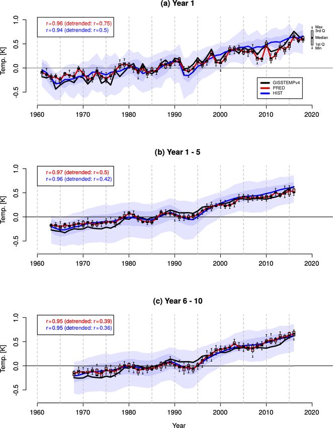
corresponds to the average of SST anomalies over the cen- When the simulations are detrended (a simple attempt to re-
tral equatorial Pacific (region 2: 10◦ S–10◦ N, 170◦ E–90◦ W) move the warming signal), PRED shows higher ACC skill
minus the average of the SST anomalies in the northwestern values than HIST, revealing the benefit of the initialization,
(region 1: 25–45◦ N, 140◦ E–145◦ W) and southwestern Pa- especially for the earlier forecast years (ACC values of 0.75
cific (region 3: 50–15◦ S, 150◦ E–160◦ W). To describe the and 0.5 in forecast year 1 for PRED and HIST respectively).
decadal variability over the Atlantic Basin, we use the AMV Comparing the intra-ensemble spread of PRED and HIST
definition from Trenberth and Shea (2006). The AMV is cal- (shown by the box-and-whisker plots for PRED and shad-
culated as the spatial average of SST anomalies over the ing for HIST in Fig. 1) shows that PRED has considerably
North Atlantic (Equator–60◦ N and 80–0◦ W) minus the spa- smaller spread even on the longer forecast times. For exam-
tial average of SST anomalies averaged from 60◦ S to 60◦ N ple, the mean intra-ensemble standard deviation of PRED
(Trenberth and Shea, 2006; Doblas-Reyes et al., 2013). In is 0.05 K, whereas it is 0.20 K for HIST for the first fore-
addition to the AMV, we also compute the subpolar North cast year. This is probably due to the initialization of PRED,
Atlantic (SPNA; 50–65◦ N, 60–10◦ W) ocean heat content in which puts the simulated internal and observed variability in
the upper 300 m (referred to as SPNA-OHC300 hereafter). phase and may also help to correct systematic errors in the
As the IPO, AMV and SPNA-OHC300 are decadal modes of model response to external forcing (e.g. Doblas-Reyes et al.,
variability, we filter out part of the interannual variability by 2013). This difference in spread remains comparable when
considering 4-year temporal averages along the forecast time the ensemble size of HIST is reduced to 10 members, i.e. the
(i.e. forecast years 1–4, 2–5, 3–6 . . . ) for these indices. same ensemble size of PRED.
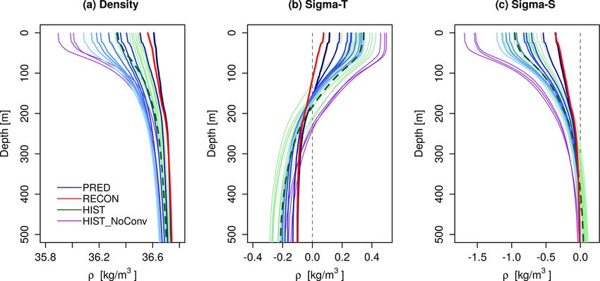
Likewise, density has been computed using the Interna-
tional Equation of State of Seawater (EOS-80) that refers to 3.1.2 Added value of initialization at the regional scale
the level of 2000 dbar (sigma-2), which is a level that rep-
resents the deep-water properties. In addition, the contribu- At the regional level, PRED shows high skill at predicting
tions of temperature (sigma-T ) and salinity (sigma-S) to den- surface temperature at different forecast ranges (Fig. 2a–c),
sity were computed using the thermal expansion and haline as expected from the presence of long-term warming trends
contraction coefficients, the latter of which were estimated (Fig. 2d–f). In the first forecast year, most regions show sig-
as the density change (in the EOS-80 equation) associated nificant skill (Fig. 2a), with a few exceptions such as the cen-
with a small increase in temperature (0.02 ◦ C) and salinity tral subpolar North Atlantic and some regions of Asia, Aus-
(0.01 psu) respectively. tralia and the Southern Ocean, where the simulated trends are
All ocean diagnostics have been computed using “Earth- small and mostly not statistically significant (Fig. 2d). By
diagnostics”, a Python-based package developed at the BSC. contrast, the eastern Pacific shows no significant trends but
does show significant skill in the first forecast year associated
with the initialization of ENSO. On longer timescales (fore-
3 Results cast ranges from 1 to 5 and 6 to 10 years) PRED also shows
significant skill in many regions worldwide with greater ACC
3.1 Characterizing the predictive capacity of surface values compared with forecast year 1 (Fig. 2b, c). This is
temperature probably a consequence of considering 5-year averages for
3.1.1 Global mean surface temperature validation, which reduces the influence of the unpredictable
part of interannual variability. There is, however, an impor-
First we compare the predicted GMST evolution for differ- tant degradation of the skill in some regions for these fore-
ent forecast periods (Fig. 1), estimated by combining SAT cast ranges, in particular in the eastern tropical Pacific, where
over land and SST over the ocean (see Sect. 2). PRED re- the model might not be representing the correct ENSO low-
produces the observed variability and shows very high ACC frequency variability, and in the North Pacific, where gen-
skill values: 0.96, 0.97 and 0.95 for forecast years 1, 1–5 erally low levels of skill have been related to model biases
and 6–10 respectively (similar values are obtained with com- in ocean mixing processes (Guemas et al., 2012). Compar-
parisons to other observational products like HadCRUT4). ing the forecast periods for years 1–5 and 6–10, two major
As expected, HIST does not capture most of the interan- differences are apparent. First, in the Southern Ocean, skill
nual variability (Fig. 1), as it is largely of internal origin and, degrades dramatically with forecast time, which is proba-
therefore, averages out by construction. Nevertheless, HIST bly associated with the development of a warm bias due to
shows very high skill (0.94, 0.96 and 0.95 for forecast years, the incorrect representation of cloud feedbacks in the region
1–5 and 6–10 respectively) associated with the global warm- (Hyder et al., 2018). Second, the central subpolar North At-
ing trend and the cooling episodes in response to the volcanic lantic seems to exhibit an opposite change in skill, from neg-
eruptions of Agung (1963), El Chichón (1982) and Pinatubo ative ACC values during the first 5 forecast years to positive
(1991). The differences in ACC skill between PRED and but insignificant ACC values in the 5 following years, which
HIST are not statistically significant, indicating that the high might reflect the recovery from an initial adjustment that af-
skill of PRED is mainly associated with the external forcings. fects the North Atlantic. This adjustment might be responsi-
Earth Syst. Dynam., 12, 173–196, 2021 https://doi.org/10.5194/esd-12-173-2021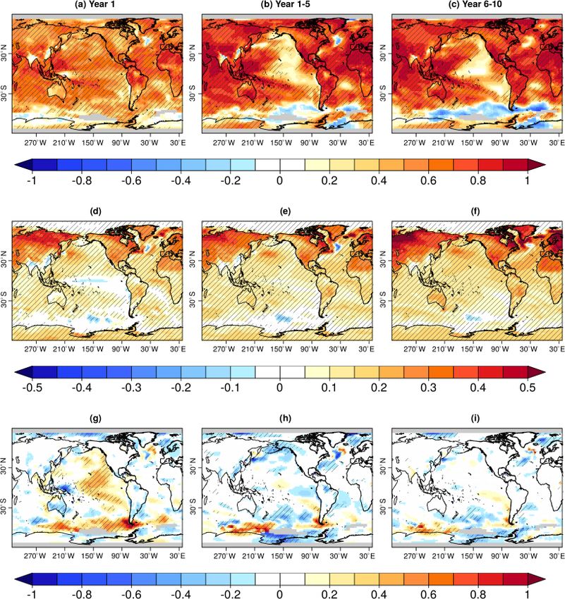
R. Bilbao et al.: EC-Earth3 decadal prediction system                                                                                     179

Figure 1. Global mean surface temperature (GMST) annual mean anomaly time series (K) for PRED, HIST (historical+SSP2-4.5) and
GISTEMPv4 for (a) forecast years 1, (b) 1–5 and (c) 6–10. The anomalies cover the 1961–2018 period and are referenced to the 1971–2000
mean. Multi-year means (b, c) are plotted on the central year (e.g. 2000 represents the values from 1998 to 2002 in panels b and c). For a fair
comparison with observations, PRED and HIST have been masked where and when GISTEMPv4 has missing values. The intra-ensemble
spread for PRED and HIST is represented by the box-and-whisker plots and shading respectively. The ACC for PRED and HIST is shown
in the top-left corner of each panel, including the ACC after removing a linear trend from the time series (shown in parentheses). All ACC
values are statistically significant at the 95 % level.

https://doi.org/10.5194/esd-12-173-2021                                                        Earth Syst. Dynam., 12, 173–196, 2021
180                                                                           R. Bilbao et al.: EC-Earth3 decadal prediction system

Figure 2. Anomaly correlation coefficient (ACC) for the annual surface temperature (SAT and SST blend) in PRED for forecast years (a) 1,
(b) 1–5 and (c) 6–10. The ACC is computed between the model ensemble mean of the blended SAT (over land) and SST (over the ocean)
fields and GISTEMPv4. Grid points with missing values in observations are masked in grey. Panels show surface temperature linear trends
(in K per decade) in PRED for the same forecast years as in panels (a–c). Panels (g–i) show the ACC difference between PRED and HIST in
the same forecast years as above. In all rows, hatching indicates significance at the 95 % confidence level. Both ACC and trends are computed
for annual mean values of all available years for the respective forecast period referenced to the 1970–2018 climatology.

Earth Syst. Dynam., 12, 173–196, 2021                                                        https://doi.org/10.5194/esd-12-173-2021
R. Bilbao et al.: EC-Earth3 decadal prediction system                                                                           181

ble for the strong negative trends over the regions in forecast   high and significant ACC values are obtained in all major
years 1–5, which are substantially reduced in forecast years      basins for the ocean heat content in the upper 300 m (referred
6–10 (Fig. 2e, f). This will be further discussed in Sect. 3.3.   to as OHC300 hereafter; Fig. 4a). A region of negative skill
    To determine whether there is a benefit of initialization     values is evident over the central subpolar North Atlantic,
on the surface temperature skill, we compute the difference       as for the surface temperatures (Fig. 2a). Forecast years 1–5
in ACC between PRED and HIST (Fig. 2g–i) as well as               and 6–10 show that the skill in the tropical and eastern Pa-
the MSSS of PRED using HIST as the reference forecast             cific is lost, as is also the case for some regions in the Atlantic
(Fig. 3a–c). Moreover, to aid in the interpretation of the        and Pacific sectors of the Southern Ocean (Fig. 4b, c). As for
MSSS values, we show the two terms that determine its sign,       surface temperature, the skill in the central subpolar North
the first being the difference between the squared ACC val-       Atlantic moderately improves in forecast years 6–10 with re-
ues of PRED and HIST (Fig. 3d–f), and the second being the        spect to forecast years 1–5.
difference between their squared conditional biases (Fig. 3g–        Comparing the ACC difference between the PRED and
i). The colour scales in all panels have been adjusted so that    HIST ensembles reveals that the initialization increases the
red colours represent a contribution to improved skill from       forecast skill of OHC300 in the eastern subpolar North At-
initialization (i.e. the colour bar was inverted for the condi-   lantic in all the three forecast times (and ranges) considered
tional bias plots).                                               (Fig. 4d–f); this is a result that is consistent with other fore-
    In the first forecast year, both ACC differences (Fig. 2g)    cast systems (e.g. Robson et al., 2018; Yeager et al., 2018).
and MSSS (Fig. 3a) show added value from initialization in        The Pacific Ocean shows significantly improved skill from
the Pacific Ocean, the neighbouring region of the Southern        initialization basin-wide in the first forecast year (i.e. ENSO);
Ocean and the eastern subpolar North Atlantic, with MSSS          however, for forecast years 1–5 and 6–10, the added value of
also showing positive impact of initialization in the subtropi-   initialization is limited to parts of the eastern subtropical Pa-
cal Atlantic. The MSSS terms reveal that in the first forecast    cific and the western tropical Pacific. The initialization im-
year, the positive MSSS values (indicative of added value of      proves the skill in most of the Indian Ocean at all forecast
initialization) are mostly associated with the squared ACC        times considered (although it is not statistically significant
term (Fig. 3d), whereas the squared conditional biases con-       for forecast years 6–10), which is consistent with previous
tribute mostly to negative MSSS skill, in particular over the     studies showing the high skill of decadal predictions in this
whole SPNA region and the northern North Pacific (Fig. 3g).       region (Guemas et al., 2013).
These negative contributions of the squared conditional bias
term are also present at forecast years 1–5, in which both        3.2   Skill for the main ocean modes of variability
the ACC and MSSS differences become predominantly neg-
ative, supporting better predictive capacity in HIST than in      We further evaluate the predictive capabilities of the EC-
PRED and, therefore, indicating that only a few areas, such as    Earth3 PRED experiment by considering the skill for pre-
the northeastern SPNA and the tropical Pacific (Fig. 3b), are     dicting several modes of interannual to decadal variability
benefiting from initialization. While the skill improvement       (Fig. 5). In the Pacific Ocean, ENSO is the main mode of
in the northeastern SPNA is clearly due the higher ACC in         climate variability on seasonal to interannual timescales and
PRED (Figs. 2h, 3e), the improvement in the tropical Pacific      can help the predictive capacity worldwide through its well-
is due to a reduction in the squared conditional bias of PRED     known climate impacts (e.g. McPhaden et al., 2006; Yuan
with respect to HIST (Fig. 3h). At longer forecast times (6–      et al., 2018). Figure 5a shows that PRED captures the year-
10 years), added value from initialization remains very lim-      to-year evolution of the observed ENSO, whereas HIST does
ited. Positive MSSS values are almost exclusive to the east-      not; this is due to the dat that ENSO events are out of phase
ern tropical Pacific and the southeastern Atlantic, due to a      across the HIST ensemble and average out. This is confirmed
reduction in the squared conditional bias in PRED with re-        by the high ACC values during the first 4 forecast months in
spect to HIST (Fig. 3i). In the northeastern SPNA, although       PRED (ACC > 0.9), which are followed by a typical loss of
the ACC is greater in PRED (Figs. 2i, 3f), the squared con-       skill that many dynamical forecast systems experience dur-
ditional bias in PRED is considerably larger than in HIST,        ing the spring season (i.e. the spring barrier; Webster and
leading to very negative MSSS values (Fig. 3i), which sug-        Yang, 1992) and by a recovery in summer through the next
gest that some regional key physical processes (e.g. the gyre     winter, in which ACC values remain positive and significant
and overturning ocean circulations) might not be well repre-      (Fig. 5b). Added value for ENSO due to initialization is evi-
sented in EC-Earth3 predictions.                                  dent up to the second forecast year, as indicated by the pos-
    To complement the analysis of surface temperature, we         itive MSSS values and the statistically significant difference
also consider the upper-ocean heat content, a quantity that       in ACC values between PRED and HIST (Fig. 5b). The lack
better represents the thermal inertia of the ocean and a source   of skill in HIST is expected, because ENSO is barely influ-
of decadal variability and predictability for the surface cli-    enced by the external forcings and the ensemble mean aver-
mate (e.g. Meehl et al., 2014; Yeager et al., 2018). As previ-    ages the phases of the individual members out. In the pre-
ously shown for surface temperature, in the first forecast year   dictions, the spread–error ratio reveals that the ENSO pre-

https://doi.org/10.5194/esd-12-173-2021                                               Earth Syst. Dynam., 12, 173–196, 2021
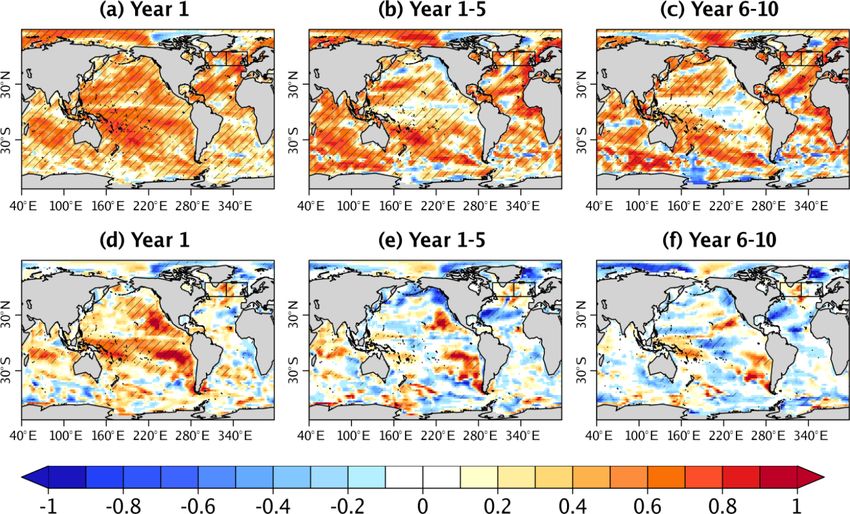
182                                                                           R. Bilbao et al.: EC-Earth3 decadal prediction system

Figure 3. Mean square skill score (MSSS) of the annual mean surface temperature (SAT and SST blend) in PRED using HIST as the reference
forecast (see Sect. 2.3) for forecast years (a) 1, (b) 1–5 and (c) 6–10. Hatching indicates where the MSSS is significant using a random walk
test (see Sect. 2.3). Its sign is determined by the difference between the terms in panels (d–f) and (g–i) (see Eq. 2). Panels (d–f) show the
difference between the squared ACC values in PRED and HIST for the same forecast years. Panels (g–i) show the difference between the
squared conditional biases in PRED and HIST for the same forecast years. Note that the colour scale in panels (g–i) is reversed with respect
to the other rows so that positive values contribute to improved skill from initialization. GISTEMPv4 is used as the observational reference
for all calculations. Annual mean anomalies are computed by masking PRED and HIST with the GISTEMPv4 missing values (masked in
grey) and using the common 1970–2018 climatology period.

Earth Syst. Dynam., 12, 173–196, 2021                                                        https://doi.org/10.5194/esd-12-173-2021
R. Bilbao et al.: EC-Earth3 decadal prediction system                                                                                     183

Figure 4. Upper 300 m ocean heat content (OHC300) anomaly correlation coefficient (ACC) of PRED computed with the EN4 observations
for (a) forecast years 1, (b) 1–5 and (c) 6–10. The impact of initialization is shown as the difference in ACC between PRED and HIST for
(d) forecast years 1, (e) 1–5 and (f) 6–10. In panels (a–c), the hatching indicates the statistical significance of the correlation at the 95 %
confidence level. For panels (d–f) hatching indicates the regions where the difference in correlation between HIST and PRED is statistically
significant at the 95 % confidence level. The black boxes in the North Atlantic delimit the region over which the SPNA indices have been
defined. It also includes the central boundary used to distinguish between its western and eastern sides.

dictions tend to be overconfident in the first 2 years, in con-           to excessive intra-ensemble spread, as previously described
trast to HIST which tends to be under-confident. On decadal               in Sect. 3.1.1.
timescales, the dominant mode of climate variability in the                  As the subpolar North Atlantic has been shown to be
Pacific Basin is the IPO. Figure 5e shows that neither PRED               a region where forecast systems exhibit skill on decadal
nor HIST is capable of skilfully predicting it – a lack of skill          timescales, we analyse the SPNA-OHC300 index (see
that has been documented in many other prediction systems                 Sect. 2.4). As for the AMV, the initialization improves the
(e.g. Doblas-Reyes et al., 2013). Nonetheless, initialization             reliability of the PRED and shows that the HIST intra-
does seem to improve the reliability of the IPO (Fig. 5f).                ensemble spread may be too large and, therefore, under-
   In the Atlantic Ocean, the AMV is the dominant mode                    confident (Fig. 5l). In terms of predictive capacity, PRED
of decadal climate variability and has been linked to sev-                exhibits a lack of skill for the SPNA-OHC300 index up to
eral climate impacts over Europe, North America and the                   the forecast range of 4 to 7 years, with significant ACC val-
Sahel (Zhang and Delwoth, 2006; Sutton and Dong, 2012;                    ues emerging for longer forecast ranges, coinciding with the
Ruprich-Robert et al., 2017, 2018) as well as to Atlantic trop-           time in which the system outperforms persistence. ACC val-
ical cyclones (e.g. Caron et al., 2015, 2018). Both PRED and              ues in the HIST ensemble (which are not statistically differ-
HIST are capable of skilfully predicting the AMV, and they                ent from those in PRED) also increase with forecast time.
show better performance than a persistence forecast (except               In HIST, this is due to the fact that the skill for each fore-
for the forecast range from 1 to 4 years in HIST), as shown               cast range is computed over a different verification period
by the ACC (Fig. 5h). PRED however, is consistently better                (the same one used for PRED), which used the longest pe-
than HIST, as shown by the MSSS, even though the ACC                      riod available for each forecast range. For the longest forecast
differences are not statistically significant. The spread–error           ranges (e.g. 7–10 years), the first start dates cannot be used,
ratio shows that initialization improves the reliability of the           thereby excluding some of the earliest years (e.g. 1960–1966;
AMV predictions at all forecast ranges (Fig. 5i), as the his-             for which the warming trend was less prominent) and, thus,
torical simulations are overdispersive, which is probably due             producing an artificial increase in skill for longer forecast

https://doi.org/10.5194/esd-12-173-2021                                                        Earth Syst. Dynam., 12, 173–196, 2021
184                                                                             R. Bilbao et al.: EC-Earth3 decadal prediction system

Figure 5. Skill of the selected modes of ocean variability: (a–c) ENSO (Niño3.4 index), (d–f) IPO, (g–i) AMV and (j–l) SPNA-OHC300.
Panels (a), (d), (g) and (j) show the observed (grey bars) and predicted (PRED in red and HIST in blue) time series of the indices. The
ensemble means are represented using lines, and the ensemble spread is shown using coloured shading. Panel (a) shows the ENSO index for
the first winter (DJF), whereas panels (d), (g) and (j) show the average of the first 4 forecast years for the other indices. Panels (b), (e), (h)
and (k) show the ACC of PRED (red) and HIST (blue), the MSSS of PRED considering HIST the baseline prediction (black dashed line) and
the ACC of a persistence forecast (purple). Statistically significant ACC values (at the 95 % confidence level) are shown using empty circles.
ACC differences that are statistically significant (at the 95 % confidence level) between the PRED and HIST are shown using filled circles.
Panels (c), (f), (i) and (l) show the spread–error ratio of PRED (red) and HIST (blue).

Earth Syst. Dynam., 12, 173–196, 2021                                                           https://doi.org/10.5194/esd-12-173-2021
R. Bilbao et al.: EC-Earth3 decadal prediction system 185
times. Repeating the calculations for PRED over a common transitions towards its free-running attractor both indices di-
verification period to all forecast ranges (i.e. 1970–2018) re- verge from RECON and experience a pronounced weaken-
veals that lower skill values are still present for the first fore- ing. By forecast year 10, the indices in PRED reach a weaker
cast years (see Fig. S1 in the Supplement), suggesting that mean state than in HIST (green dashed lines in Fig. 6c and
the differences in skill with forecast time are not due to dif- d respectively). These differences between PRED and HIST
ferences in the verification period but to other causes. If we suggest either that the forecasts in PRED need to be run
determine the skill in OHC300 in the western and eastern for longer to reach their attractor (i.e. HIST) (e.g. Sanchez-
SPNA separately (see Fig. S2), we can then see that the skill Gomez et al., 2016) or that more than one model attractor
in PRED is initially poor and then gradually increases reach- exists.
ing significant values in the last forecast years in the western For both indices, we also note a clear difference in the way
SPNA, whereas the eastern SPNA maintains a high and rela- the forecast transitions to the model attractor before and af-
tively stable predictive skill. The poor initial predictive skill ter year 2000. For the first 30 start dates, the AMOC45N and
in the western SPNA might arise from a potential initializa- NASPG in PRED start at stronger values than HIST (c.f. RE-
tion shock, which is a possibility that is discussed in the next CON values in Fig. 6a and b), and the individual predictions
subsection. The final skill recovery in the region might be re- exhibit a fast decline that surpasses the HIST mean state. In
lated to the arrival of OHC anomalies from the eastern SPNA, year 1995 of RECON, both indices experience a sharp de-
which are slowly advected by the mean gyre circulation. crease and eventually stabilize around a substantially lower
mean state, which is a transition that has been shown to be
3.3 Understanding the limited predictive skill in the
partly predictable in previous studies (Robson et al., 2012;
subpolar North Atlantic
Yeager et al., 2012; Msadek et al., 2014). Due to this weaker
initial state, all predictions after the year 2000 start much
In the previous section, we have shown the overall detri- closer to the HIST mean state. As a consequence, the drift in
mental effect of initialization in the EC-Earth3 predictions PRED is smoother for this period. The fact that there are two
over some regions of the North Atlantic at all forecast ranges distinct periods in which the model drifts in different ways
(Fig. 3), leading to lack of predictive skill in the specific (Fig. 6c, d) may compromise the applicability of the drift
case of the central subpolar North Atlantic, as shown by the correction methods used to compute the forecast anomalies,
ACC maps of surface temperature (Fig. 3) and upper-ocean which assume a stationary forecast drift. This is particularly
heat content (Figs. 4, 5). Decadal variability in the subpo- evident for the AMOC45N, which shows important differ-
lar North Atlantic is highly influenced by the changes in the ences in the PRED climatologies during the first 3 forecast
ocean circulation, both meridional and barotropic (e.g. Or- years when the climatologies are computed for the time pe-
tega et al., 2017). To understand the role of the ocean circu- riods preceding and following the year 2000 (Fig. 6c red and
lation, we analyse the evolution of the Atlantic Meridional blue lines respectively). Thus, in the case of the AMOC, ap-
Overturning Circulation at 45◦ N (defined as the overturn- plying the standard mean drift correction leads to an under-
ing stream function value at 45◦ N and at 1000 m depth; re- estimation of its intensity over the first period and an over-
ferred to as AMOC45N hereafter) and North Atlantic Subpo- estimation over the second period within the first 3 forecast
lar Gyre strength index (NASPG, defined as the regional av- years. In light of this problem, refining the current drift cor-
erage of the barotropic stream function in the Labrador Sea rection techniques to account for this sensitivity to the period
(52–65◦ N, 58–43◦ W), multiplied by minus one to make the and/or initial state considered, or exploring other alterna-
values positive so as to aid the comparison) in PRED and tive statistical drift models to recalibrate the predictions (e.g.
HIST (Fig. 6a , b). Additionally, we include the ocean-only Nadiga et al., 2019) might help to better estimate the true pre-
reconstruction from which the initial conditions are obtained diction skill. Interestingly, other variables like the NASPG
(referred to as RECON hereafter) to determine how the pre- seem to be less affected by non-stationary drifts (Fig. 6d).
dictions depart from the initial conditions. Actual model val- To understand why the AMOC45 and NASPG are not sta-
ues are used to illustrate how the forecast drift develops. bilizing in the predictions around the mean HIST state, we
The mean forecast drift is also shown for completeness, es- focus on the Labrador Sea. The Labrador Sea is a key re-
timated as the climatological value as a function of forecast gion of deep-water formation, in which climate models show
time (Fig. 6c, d). Figure 6 shows that decadal changes in the limitations with respect to representing realistic oceanic con-
AMOC and NASPG are highly correlated (e.g. R = 0.8 in vection, which can happen too often, too deep or can be com-
RECON) – a relationship that has been shown in previous pletely absent in some cases (Heuzé, 2017). Figure 7a shows
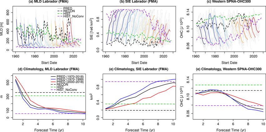
studies (Ortega et al., 2017). the mixed layer depth (MLD) evolution in the Labrador Sea,
Comparing PRED and RECON allows us to identify sev- which is a proxy for the convection activity in this region.
eral interesting features. In the first forecast year, the pre- The MLD index is computed as the average of February–
dicted AMOC45N is of equal value with respect to RE- March–April, which are the months with the deepest mix-
CON, whereas the predicted values tend to be weaker for the ing. In PRED, MLD systematically collapses within the first
NASPG index (Fig. 6). As the forecasts evolve and the model 3 forecast years, which is in stark contrast with the typical
https://doi.org/10.5194/esd-12-173-2021 Earth Syst. Dynam., 12, 173–196, 2021186 R. Bilbao et al.: EC-Earth3 decadal prediction system
Figure 6. Evolution of the (a) AMOC45N and (b) NASPG in the raw forecasts, historical ensemble and reconstruction. Ensemble mean
forecasts (10 members) of PRED are shown from blue to red every four start dates, with individual ensemble members shown in grey.
The ensemble mean RECON (5 members) is shown with the black dashed line. The ensemble mean of all HIST (15 members) is shown
in green, and the ensemble mean of the HIST members that do not exhibit convection are shown in purple. Panels (c, d) show the PRED
climatological values as a function of forecast time for the AMOC45N and NASPG respectively. Three time periods are considered for
PRED: the climatology for the 1970–2018 period (black), the climatology for the 1970–2000 period (red) and the climatology for the 2000–
2018 period (blue). The black, green and purple dashed lines indicate the climatology computed over the 1970–2018 period for RECON, all
HIST members, and HIST members that do not show convection respectively.
behaviour in the HIST ensemble, in which deep convection in PRED, which initially boosts convection and subsequently
happens regularly. In the HIST ensemble mean, Labrador brings the model towards a non-convective mean state.
convection remains active throughout the whole period, al- Other key indices are also affected by the Labrador Sea
though it exhibits a long-term weakening trend, consistent convection collapse in PRED. For example, we see that sea
with the increase in local stratification caused by the exter- ice grows to occupy the whole Labrador Sea as soon as con-
nally forced ocean surface warming. The Labrador MLD in- vection ceases (Fig. 7b, e). As for the MLD, the sea ice ex-
dex also allows us to identify three HIST members with a tent of the HIST members with no convection is remarkably
distinct evolution from the rest, characterized by no convec- similar, whereas convection in the other members maintains
tion during most of the historical period with a slight increase a relatively reduced sea ice coverage. The western SPNA-
from 2005 onward (purple line in Fig. 7a). These simula- OHC300 (50–65◦ N, 60–30◦ W) also seems to experience an
tions have a remarkable similarity to the state towards which abrupt initial change, as shown in Fig. 7c; the PRED cli-
PRED appears to be drifting. The ensemble mean of these matological value at a forecast time of 1 year is lower than
three HIST members is also compatible with the AMOC45N in the RECON climatology (Fig. 7f). In forecast years 2–
and NASPG states at the end of the forecasts (purple lines 3, this index tends to increase, approaching the HIST mean
in Fig. 6), suggesting that the attractor towards which PRED state, which is higher than in RECON. However, this trajec-
converges is associated with a suppressed Labrador Sea con- tory changes drastically after forecast year 3 (Fig. 7f), and a
vection state. Note also that, in the first forecast year of quick cooling begins towards the no-convection HIST state.
PRED, the Labrador Sea MLD is stronger than in RECON. This sudden change could be explained by a delayed re-
All of the above suggest the existence of an initial adjustment sponse to the convection collapse in the predictions, which
is expected to drive a weakening of the SPG intensity by
Earth Syst. Dynam., 12, 173–196, 2021 https://doi.org/10.5194/esd-12-173-2021You can also read